A Cellular Automata Study of Constraints (Dissolvence) in a Percolating Many-Particle System

Abstract

In a recent study by Kier, Cheng and Testa, simulations were carried out to monitor and quantify the emergence of a collective phenomenon, namely percolation, in a many-particle system modeled by cellular automata (CA). In the present study, the same set-up was used to monitor the counterpart to collective behavior, namely the behavior of individual particles, as modeled by occupied cells in the CA simulations. As in the previous study, the input variables were the concentration of occupied cells and their joining and breaking probabilities. The first monitored attribute was the valence configuration (state) of the occupied cells, namely the percent of occupied cells in configuration F_i (%F_i), where i = number of occupied cells joined to that cell. The second monitored attribute was a functional one, namely the probability (in %) of a occupied cell in configuration F_i to move during one iteration (%M_i).

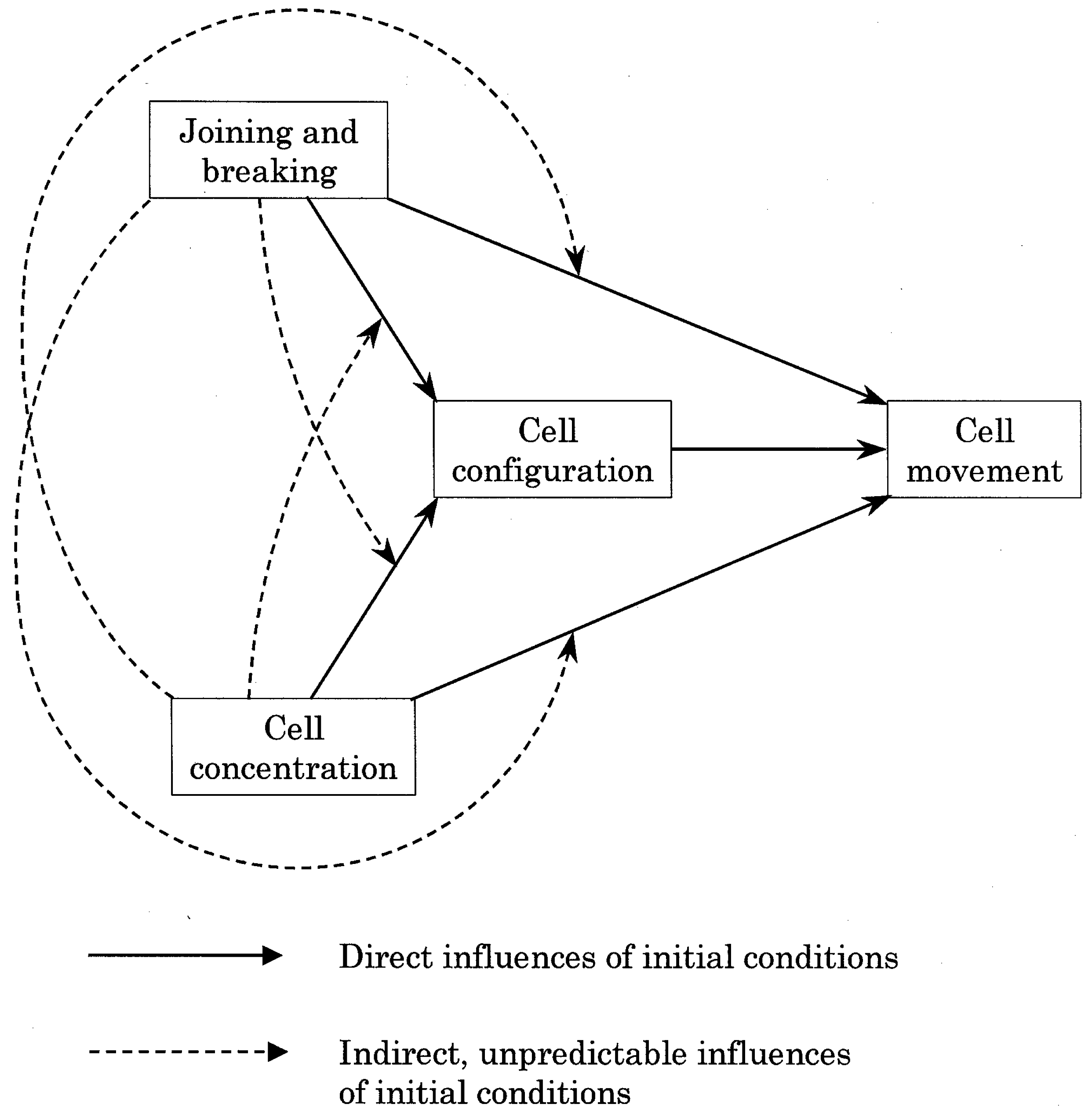
First, this study succeeded in quantifying the expected, strong direct influences of the initial conditions on the configuration and movement of occupied cells. Statistical analyses unveiled correlations between initial conditions and cell configurations and movements. In particular, the distribution of configurations (%F_i) varied with concentration with a kinematic-like regularity amenable to mathematical modeling. However, another result also emerged from the work, such that the joining, breaking and concentration factors not only influenced the movement of occupied cells, they also modified each other's influence (Figure 1). These indirect influences have been demonstrated quite clearly, and some partial statistical descriptions were established. Thus, constraints at the level of ingredients (dissolvence) have been characterized as a counterpart to the emergence of a collective behavior (percolation) in very simple CA simulations.

Introduction

Cellular automata are dynamical computational systems that are discrete in space, time and configuration and whose behavior is determined completely by rules governing local relationships. As an approach to the modeling of emergent properties of complex systems, cellular automata have the great interest of being visually informative of the progress of dynamic events [1]. From the early development by von Neumann [2] a variety of applications ranging from gas phenomena to biological applications have been reported [3]. We view cellular automata as an opportunity to advance our understanding of the dynamic behavior of probabilistic systems and have embarked upon a series of studies with this goal in mind.

In a recent study, a dynamic model of the percolation process in a many-particle system was created using cellular automata [4]. Percolation is a phenomenon associated with ingredients in a system reaching a critical state of association so that information may be transmitted across or through the system without interruption. Percolation is both a structural feature of the entire system and a process found throughout chemistry (as in the case of polymer and gel formation [5,6,7,8]) and biology (as in self-assembly of virus molecules and agglutination phenomena [9]). In cellular automata, percolation is reached when a single cluster is formed which traverses the entire system, allowing an uninterrupted flow of information across the system.

Our study [4] showed the ability of cellular automata to model the dynamic events leading to the emergence of percolation. The concentrations of occupied cells in a grid were determined for the onset and for the 50% probability of percolation occurring. The valence configuration of the occupied cells (i.e., their being joined to 0, 1, 2, 3 or 4 occupied cells) at various concentrations was analyzed to reveal a pattern of diversity. The Shannon information content for each concentration correlated very closely with the concentration of divalent cells.

This study reinforced our belief in the ability of cellular automata to model the emergence of properties of a higher order of complexity from an ensemble of systems of lower order. Furthermore, there arose from such studies the possibility of simulating another process, coexisting with emergence. That is the process we have called dissolvence [10,11,12], a counterpoint to the process of emergence in the formation of a complex system. When the coupling of ingredients M forms a system M+1 of higher level, these ingredients experience constraints such as a decline in their choices, options, and independence. In other words, there is a reduction in the number of formal and functional states accessible to them, as they become engaged in the transactions that create the higher system M+1 and its emergent properties [1,12,13,14]. This is seen in the reduction of the property space of atoms when they merge to form molecules, of amino acids when they form proteins, and in biomacromolecules when they form aggregates such as molecular machines or membranes. For reasons of parity with emergence, the word dissolvence has been proposed to describe such a phenomenon [10].

This aspect of the dynamic simulation of emergence has been largely ignored in physical, chemical and biological systems, indeed in almost all of the studies of dynamic processes. Recent computational studies have shown how the incorporation of amino acids into peptides is accompanied by constraints on their property space, a poorly recognized phenomenon of potential biological and pharmacological significance [15,16]. An understanding of the process called dissolvence could lead to better prediction of future events and rational molecular design.

Figure 1. Schematic representation of the known and postulated influences of initial conditions on occupied cell configuration (patterns of association) and occupied cell movement (probability to move). The expected, direct influence of initial conditions on occupied cell configuration and movement are represented as full arrows. The postulated, unpredictable constraints imposed on occupied cells should be detectable as indirect influences, namely initial conditions modulating each other's influence (broken arrows).

Figure 1. Schematic representation of the known and postulated influences of initial conditions on occupied cell configuration (patterns of association) and occupied cell movement (probability to move). The expected, direct influence of initial conditions on occupied cell configuration and movement are represented as full arrows. The postulated, unpredictable constraints imposed on occupied cells should be detectable as indirect influences, namely initial conditions modulating each other's influence (broken arrows).

These considerations led us to revisit our cellular automata simulations of the percolation process [4], using the same setup, for a possible identification of dissolvence in the behavior of individual particles in a many-particle system. In such simulations, dissolvence should appear in the form of constraints on the individual cells, not predictable from the initial conditions (i.e., from concentration of occupied cells and particularly from the rules of joining and breaking). To this end, we have examined in this study the influence of initial conditions on two attributes of individual, occupied cells, namely their form and function (Figure 1). The attribute of form was taken as the valence configuration of occupied cells. The functional attribute was the probability of movement experienced by the occupied cells at each iteration. The expected, direct influence of concentration and rules on the configuration and movement of occupied cells are represented as full arrows in Figure 1. In contrast, there is no way to predict if and how the concentration in occupied cells should modulate the influence of the joining and breaking rules, and how the latter should modulate the influence of concentration. Such indirect effects are depicted as broken arrows in Figure 1. We reasoned that should these indirect effects be characterized, they would represent unpredictable constraints experienced by the occupied cells.

The first objective of this study was to quantify the expected, strong direct influences of the initial conditions on the configuration and movement of occupied cells. The second objective was to find correlations between initial conditions and output. The ultimate objective was the search for indirect (and unpredictable) constraints suggestive of additional influences. All three objectives have been met, and most notably the third one. In other words, constraints (dissolvence) at the level of ingredients (individual particles) have been characterized in simulations of a many-particle system evolving toward an emergent property (in this case percolation).

Methods

The model

Our model is composed of a grid of cells. Each cell has four adjoining neighbors and four extended neighbors beyond these. These eight cells make up an extended von Neumann neighborhood. Each cell can be empty or occupied. At each iteration, an occupied cell having an empty extended von Neumann neighborhood will move by one cell either up, down, right or left. When its extended von Neumann neighborhood is not empty, an occupied cell may break away from a neighboring cell or move to join another occupied cell. These movements are governed by probabilistic rules of breaking and joining (see next paragraph) set at the beginning of the dynamics to reflect a relationship among the ingredients in the system.

The rules

Two parameters were adopted in our model to govern the probabilities of occupied cells moving and interacting. The breaking probability, P_B, is the probability for an occupied cell to break away from a cluster. The value for P_B lies from zero to one. The second parameter is the joining parameter J, which describes the movement of an occupied cell toward or away from another occupied cell from which it is separated by one empty cell. J is a positive real number. When J = 1, it indicates that the occupied cell has a neutral probability of movement toward or away from the other occupied cell. When J > 1, it indicates that the occupied cell has a greater probability of movement toward (i.e. joining) the other occupied cell, whereas the opposite is true when J < 1.

These rules are applied uniformly to each occupied cell in turn, selected randomly, until all occupied cells have computed their movement. This is one iteration of time. The initial state of the system is random hence it does not determine subsequent configurations at any iteration. The same set of rules do not yield the same configurations except in some average sense. The configurations after many iterations reach a collective organization that possesses a relative constancy in appearance and in reportable attributes of occupied cells. These are the emergent characteristics of many-particle complex systems which are explored here.

Study design and cell properties monitored

The study was made using 3025 cells in a 55×55 grid. The grid was the surface of a torus to eliminate boundary conditions. Cells in varying number were filled, the number of occupied cells ranging from 100 (concentration C = 100/3025 = 0.03306) to 2500 (C = 0.8264). These occupied cells moved randomly and interacted according to rules to join another occupied cell (joining parameter J), or break from another joined occupied cell (breaking probability P_B). Nine sets of the J and P_B parameters (Table 1), combined with a range of concentrations were employed to discover the influence of these conditions on occupied cell behavior and attributes monitored individually. Thus, Set 3 corresponds to a condition of high affinity between occupied cells (low breaking and high joining probabilities), whereas the opposite condition is true of Set 7. Set 5 corresponds to a medium affinity (intermediate breaking and joining probabilities). Extreme cases are explored with, e.g., Set 1 (low breaking and low joining) and Set 9 (high breaking and high joining).

Table 1. Joining and Breaking Parameters, and the Emergence of Percolation.

Parameter set	Joining parameter J	Breaking probability PB	C50%a)
1	0.50	0.25	0.503
2	1.50	0.25	0.488
3	3.00	0.25	0.476
4	0.50	0.50	0.546
5	1.50	0.50	0.530
6	3.00	0.50	0.519
7	0.50	0.75	0.573
8	1.50	0.75	0.559
9	3.00	0.75	0.558

a) Concentration of occupied cells corresponding to a 50% probability of percolation [4].

Table 1. Joining and Breaking Parameters, and the Emergence of Percolation.

Parameter set	Joining parameter J	Breaking probability PB	C50%a)
1	0.50	0.25	0.503
2	1.50	0.25	0.488
3	3.00	0.25	0.476
4	0.50	0.50	0.546
5	1.50	0.50	0.530
6	3.00	0.50	0.519
7	0.50	0.75	0.573
8	1.50	0.75	0.559
9	3.00	0.75	0.558

a) Concentration of occupied cells corresponding to a 50% probability of percolation [4].

The first attribute monitored was a contextual one, namely the configuration of an occupied cell (F_i; i = 0, 1, 2, 3, 4), also called state, where i = number of occupied cells joined to that cell. The percent of occupied cells in configuration F_i is expressed as %F_i. The second attribute was a functional one, namely the probability (in %) of a occupied cell in configuration F_i to move during one iteration (%M_i).

Two studies were carried out which differed in design and objective. The first study (Study A) aimed at recording the average percent of occupied cells in each of the five configurations F_i (%F_i), as influenced by the concentration and the joining and breaking parameters. Here, the number of occupied cells in each configuration (F₀, F₁, F₂, F₃, F₄) was counted after each iteration and averaged over 100 iterations. The results (%F_i) were not influenced by the number of iterations preceding the 100 monitored ones, and they remained consistent (within 1-2%) after a larger number of iterations.

The second study (Study B) aimed at recording the movements of a single occupied cell at each iteration, as influenced by the concentration and the joining and breaking parameters. Here, a single, selected occupied cell (i.e., a particle) was monitored during ten runs of 3000 iterations each. At each iteration, the program recorded a) the configuration (F_i) of this occupied cell before computing its movement, and b) whether it had moved or not. At the end of the 10 runs of 3000 iterations, the program reported the number of times the occupied cell had been in each configuration F_i (%F_i), and the number of times it had moved when in configuration F₀, F₁, F₂, F₃ and F₄ (%M_i). It was found that for the same set of conditions (concentration, P_B and J), %F_i was similar (within 1-2 %) whether it was determined in Study A (where all occupied cells were monitored over 100 iterations) or in Study B (where a single occupied cell was monitored over 10 runs of 3000 iterations each).

Programs

The cellular automata simulations were run using the program DING-HAO as described [17,18,19,20,21]. Kinetic and statistical calculations were run with the programs Kinetica 2.0 (Innaphase, Champs-sur-Marne, France) and an MS Excell Add-In [22], respectively.

Results and Discussion

Study A: Average percent of occupied cells in each configuration (%F_i)

Descriptive approach

In a first approach, it was necessary to examine whether and how the distribution of configurations would be influenced by the concentration and the joining and breaking probabilities. The simulations were run for all nine sets of joining and breaking probability (Table 1), at four concentrations: C = 0.0826 (250 occupied cells/3025 cells), C = 0.1653 (500 occupied cells/3025 cells), C = 0.3306 (1000 occupied cells/3025 cells) and C = 0.6612 (2000 occupied cells/3025 cells).

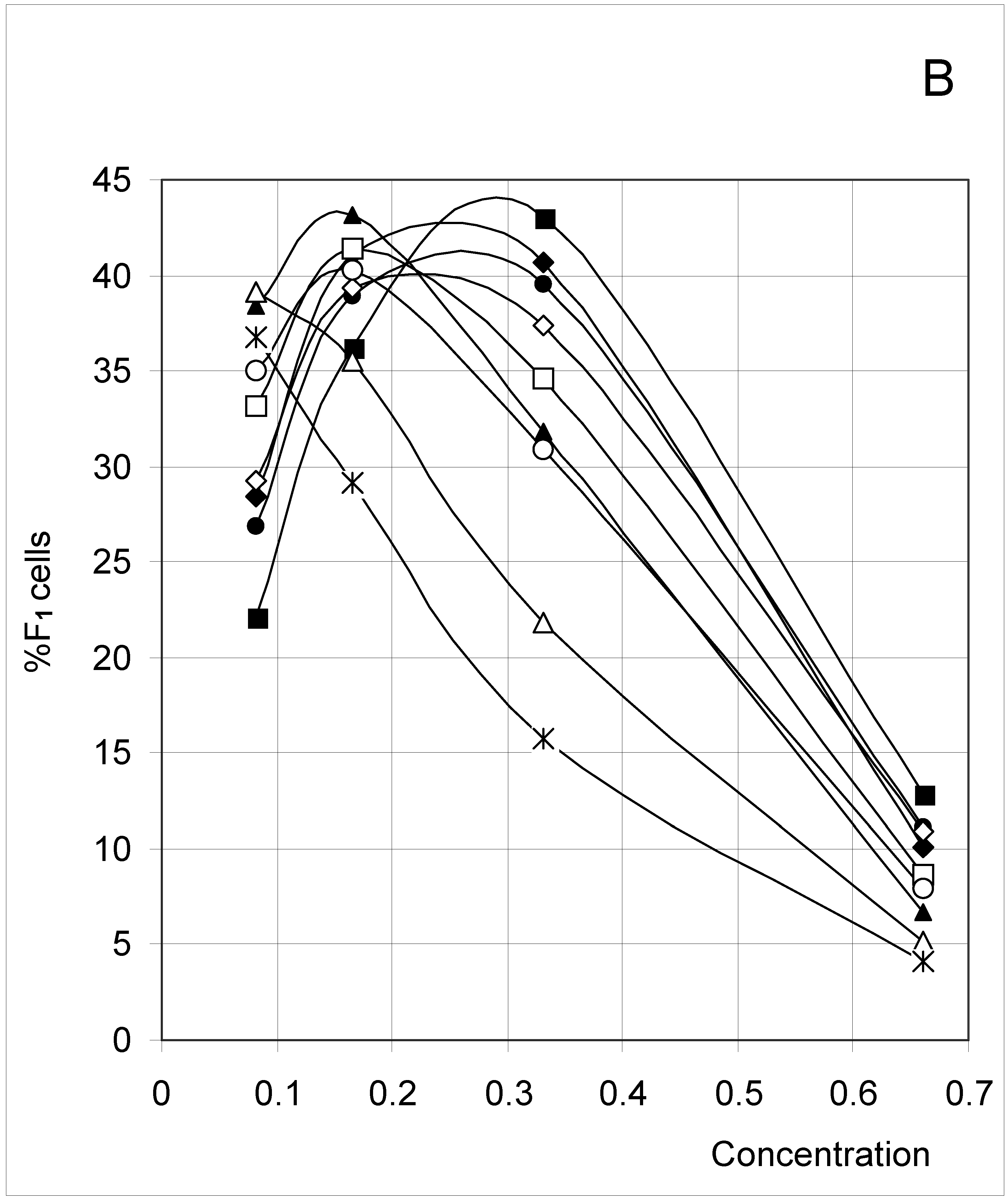
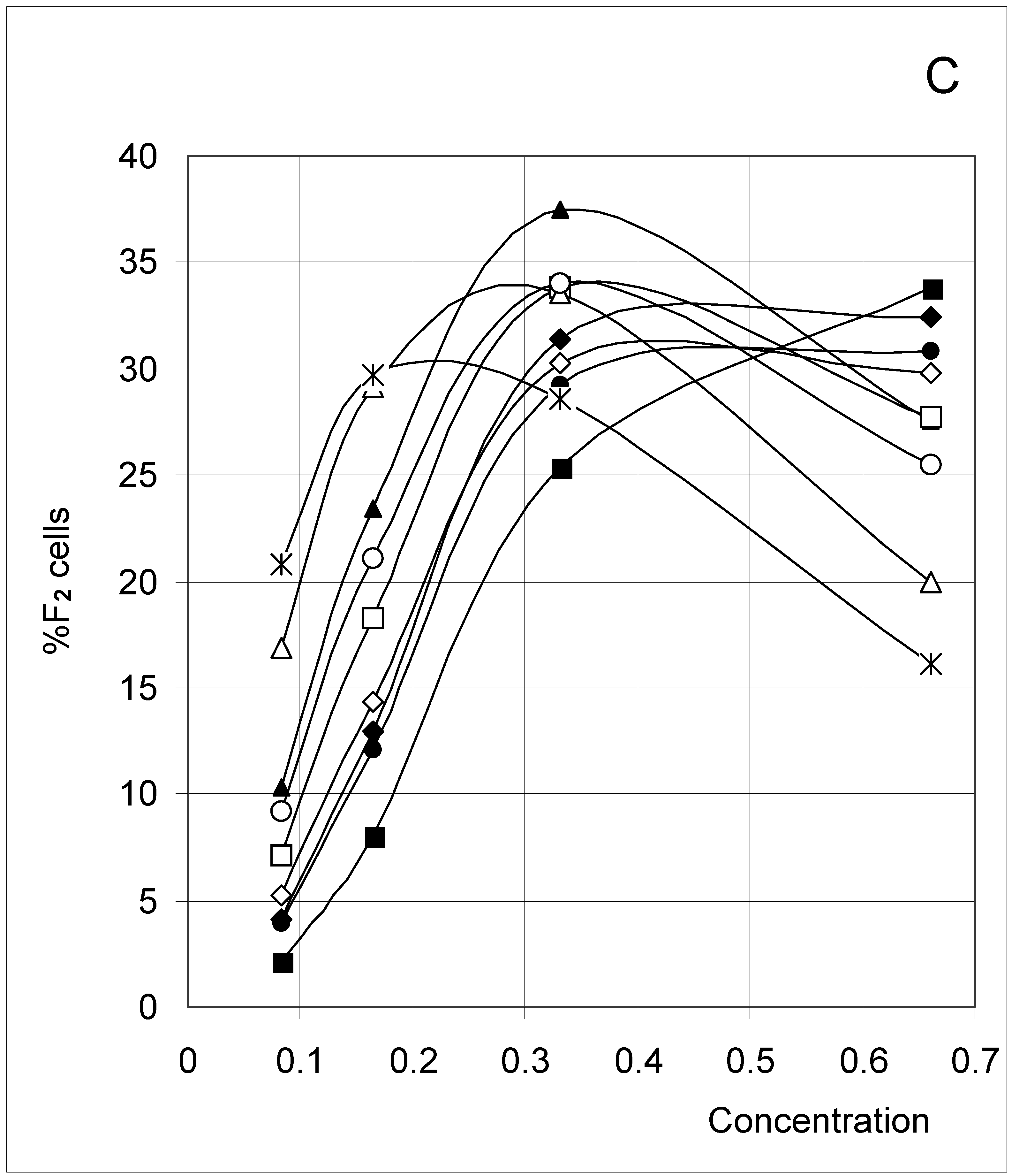
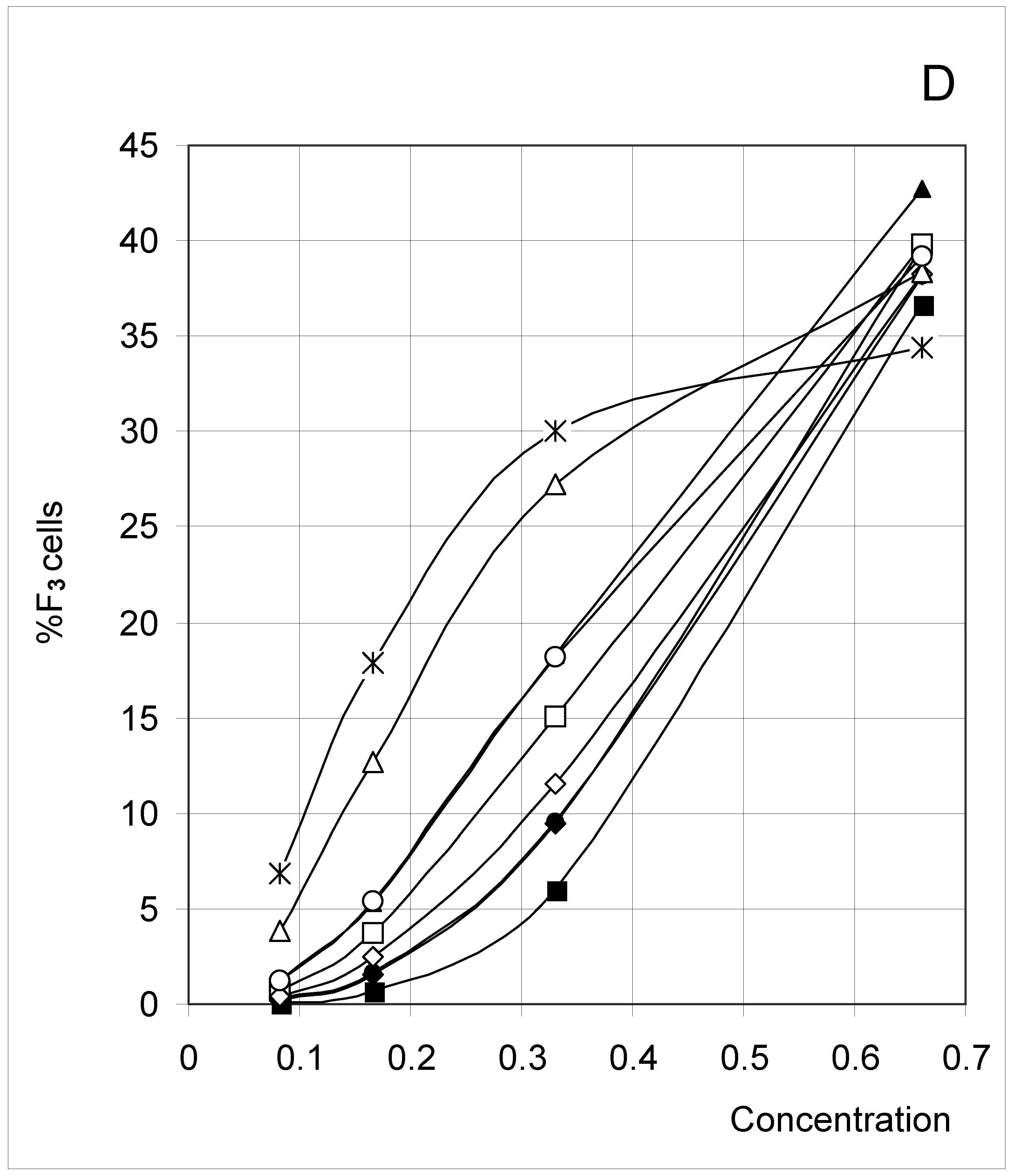
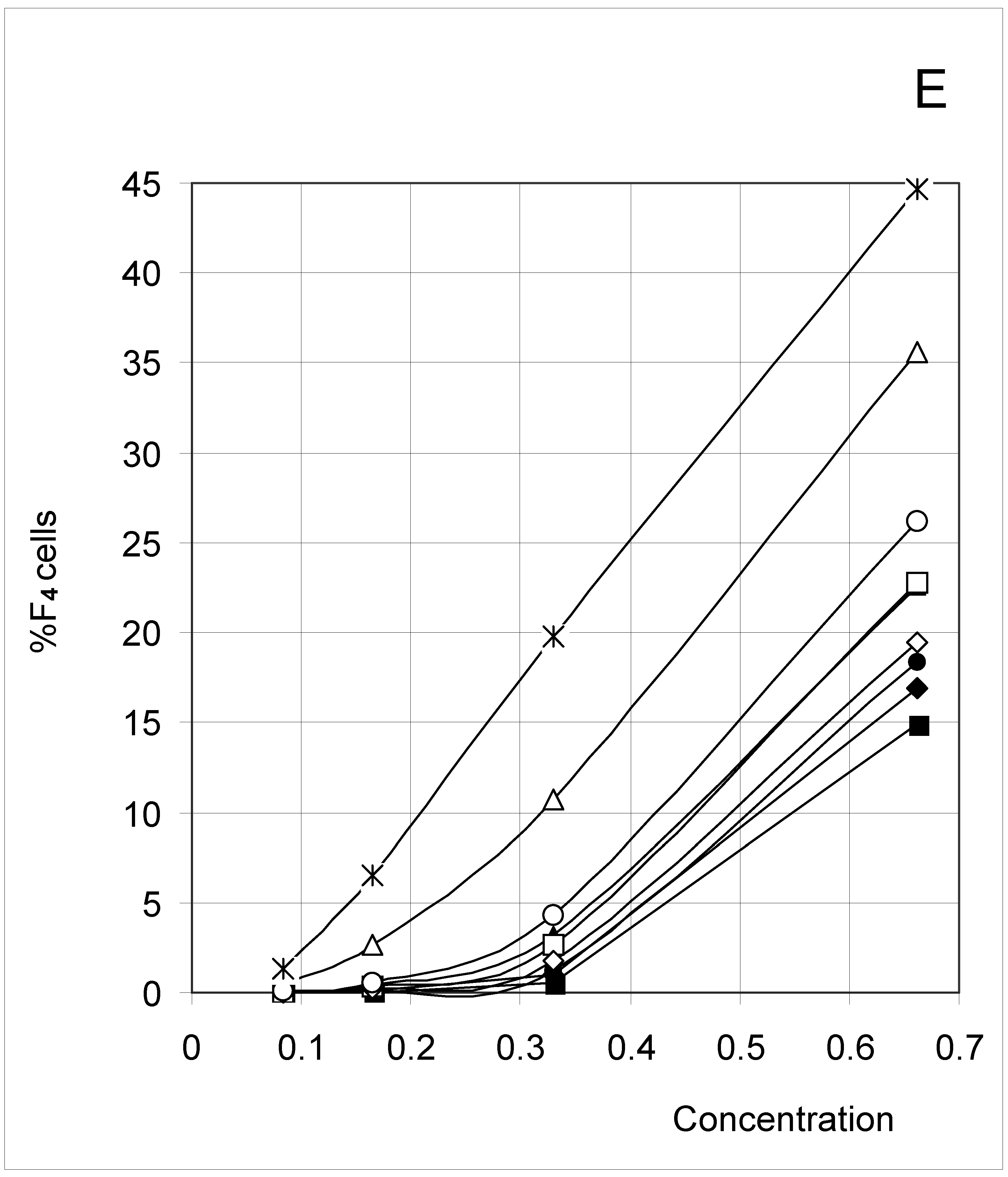
The results (Figure 2) clearly indicate a decrease in %F₀ (Figure 2A) with increasing concentration, but an increase in %F₃ (Figure 2D) and %F₄ (Figure 2E). The percent of F₁ cells (Figure 2B) showed a tendency to decrease with concentration, except at low concentrations. In contrast, the percent of F₂ cells increased with concentration (Figure 2C), except at high concentrations. These trends confirm for an extended set of conditions the observations previously published [4]. The highest affinity between occupied cells (high J and low P_B, Set 3) corresponds to the lowest %F₀ and highest %F₄ values, whereas the opposite is true for the lowest affinity between occupied cells (low J and high P_B, Set 7). A median affinity (Set 5) yielded intermediate %F₀ and %F₄ values.

Figure 2A. Distribution of occupied F₀ cells (%F₀ cells) as a function of predetermined conditions. The joining probability (J) and breaking probability (P_B) are as follows: ▲ = Set 1; ∆ = Set 2; * = Set 3; ◆ = Set 4; □ = Set 5; ○ = Set 6; ■ = Set 7; ● = Set 8; ◇ = Set 9.

Figure 2A. Distribution of occupied F₀ cells (%F₀ cells) as a function of predetermined conditions. The joining probability (J) and breaking probability (P_B) are as follows: ▲ = Set 1; ∆ = Set 2; * = Set 3; ◆ = Set 4; □ = Set 5; ○ = Set 6; ■ = Set 7; ● = Set 8; ◇ = Set 9.

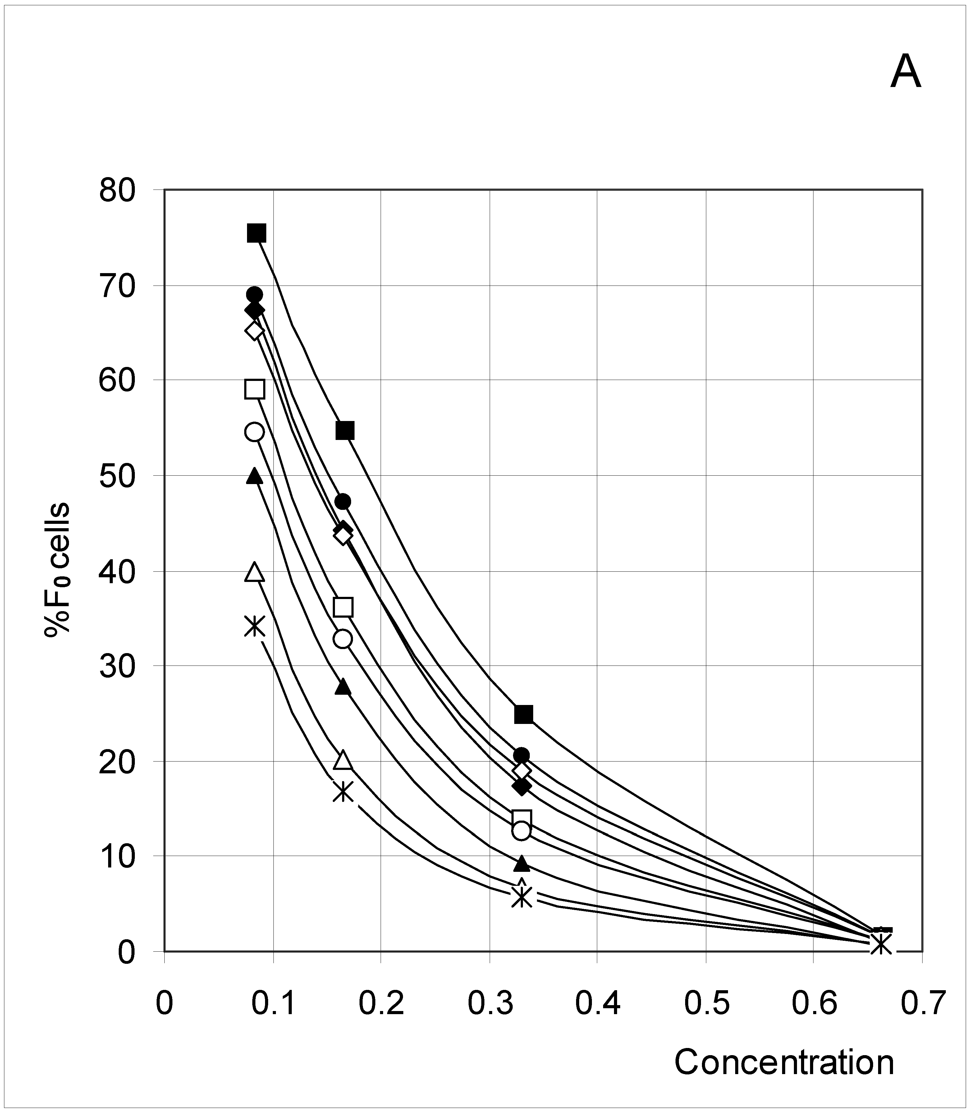
Figure 2B. Distribution of occupied F₁ cells (%F₁ cells) as a function of predetermined conditions. The joining probability (J) and breaking probability (P_B) are as follows: ▲ = Set 1; ∆ = Set 2; * = Set 3; ◆ = Set 4; □ = Set 5; ○ = Set 6; ■ = Set 7; ● = Set 8; ◇ = Set 9.

Figure 2B. Distribution of occupied F₁ cells (%F₁ cells) as a function of predetermined conditions. The joining probability (J) and breaking probability (P_B) are as follows: ▲ = Set 1; ∆ = Set 2; * = Set 3; ◆ = Set 4; □ = Set 5; ○ = Set 6; ■ = Set 7; ● = Set 8; ◇ = Set 9.

Figure 2C. Distribution of occupied F₂ cells (%F₂ cells) as a function of predetermined conditions. The joining probability (J) and breaking probability (P_B) are as follows: ▲ = Set 1; ∆ = Set 2; * = Set 3; ◆ = Set 4; □ = Set 5; ○ = Set 6; ■ = Set 7; ● = Set 8; ◇ = Set 9.

Figure 2C. Distribution of occupied F₂ cells (%F₂ cells) as a function of predetermined conditions. The joining probability (J) and breaking probability (P_B) are as follows: ▲ = Set 1; ∆ = Set 2; * = Set 3; ◆ = Set 4; □ = Set 5; ○ = Set 6; ■ = Set 7; ● = Set 8; ◇ = Set 9.

Figure 2D. Distribution of occupied F₃ cells (%F₃ cells) as a function of predetermined conditions. The joining probability (J) and breaking probability (P_B) are as follows: ▲ = Set 1; ∆ = Set 2; * = Set 3; ◆ = Set 4; □ = Set 5; ○ = Set 6; ■ = Set 7; ● = Set 8; ◇ = Set 9.

Figure 2D. Distribution of occupied F₃ cells (%F₃ cells) as a function of predetermined conditions. The joining probability (J) and breaking probability (P_B) are as follows: ▲ = Set 1; ∆ = Set 2; * = Set 3; ◆ = Set 4; □ = Set 5; ○ = Set 6; ■ = Set 7; ● = Set 8; ◇ = Set 9.

Figure 2E. Distribution of occupied F₄ cells (%F₄ cells) as a function of predetermined conditions. The joining probability (J) and breaking probability (P_B) are as follows: ▲ = Set 1; ∆ = Set 2; * = Set 3; ◆ = Set 4; □ = Set 5; ○ = Set 6; ■ = Set 7; ● = Set 8; ◇ = Set 9.

Figure 2E. Distribution of occupied F₄ cells (%F₄ cells) as a function of predetermined conditions. The joining probability (J) and breaking probability (P_B) are as follows: ▲ = Set 1; ∆ = Set 2; * = Set 3; ◆ = Set 4; □ = Set 5; ○ = Set 6; ■ = Set 7; ● = Set 8; ◇ = Set 9.

In the case of %F₁ (Figure 2B), the highest affinity between occupied cells (high J and low P_B, Set 3) produced a regular decrease with increasing concentration. In contrast, the lowest affinity (low J and high P_B, Set 7) produced a bell-shaped variation. In fact, this type of variation has been seen for seven sets, with the maximum being shifted to higher concentrations as affinity decreased.

A comparable trend has been seen for %F₂ (Figure 2C), where most sets yielded a bell-shaped variation (bearing some resemblance to a parabola) whose maximum was shifted to higher concentrations as inter-cell affinity decreased. In the percent of F₃ cells (Figure 2D), there was a regular increase with concentration comparable to %F₄, with the exception of Set 3 (low affinity) where part of a bell-shaped relation was apparent.

Correlations between initial conditions and configuration of occupied cells

In the above interpretion, Figure 2A, Figure 2B, Figure 2C, Figure 2D and Figure 2E confirm that the percent of F₀, F₁, F₂, F₃ and F₄ varied in a understandable and predictable manner with concentration and with the joining and breaking probabilities. Because such a conclusion is a qualitative one, we searched for some quantitative insights.

In a first approach, we examined how some %F_i values were correlated with concentration (C), joining (J) and breaking (P_B). Some significant correlations were found, as reported in equation 1 (which contains all 36 points in Fig. 2A) and equation 2 (which contains all 36 points in Fig. 2D):

%F₀ = 41.0(±5.2) C² − 60.3(±5.2) C − 2.91(±1.01) J + 7.33(±1.01) P_B + 27.2(±1.0)

(1A)

%F₀ = 1.74 C²− 2.55 C − 0.123 J + 0.310 P_B

(1B)

n = 36; r² = 0.944; s = 5.96; F = 129.7

%F₃ = 14.5(±0.6) C + 1.47(±0.64) J − 3.21(±0.64) P_B + 15.5(±0.6)

(2A)

%F₃ = 0.944 C + 0.096 J − 0.209 P_B

(2B)

n = 36; r² = 0.944; s = 3.82; F = 178.6

Here and below, each equation is presented in direct form (equations A), then in normalized for (equations B) where the regression coefficients reflect the relative contribution of each independent variable and the intercept is zero. In these and the following equations, the standard error of each regression coefficient is given in parenthesis, r² is the squared correlation coefficient, s the standard error of the equation, and F is Fischer's test.

%F₀ (Eq. 1) is an apparent parabolic function of concentration, whereas for %F₃ the relation with concentration is linear (Eq. 2). Eq. 1 also show that %F₀ decreased with joining and increased with breaking, whereas %F₃ increased with joining and decreased with breaking. The multiple linear regressions for %F₁ (Fig. 2B), %F₂ (Fig. 2C) and %F₄ (Fig. 2E) were of lesser statistical significance and are not reported. As seen in the corresponding Figures, the function relating conditions and output appears much more complex for these configurations. Nevertheless, Eq. 1 and 2 show that a statistically describable relation exists, at least in some cases, between configuration (%F_i) and initial conditions (concentration, joining and breaking).

Kinematic-like description

In another approach to find quantitative insights, simulations were run for 25 concentrations and three sets of joining and breaking probabilities. The 25 selected concentrations were regularly distributed between C = 0.03306 (100 occupied cells/3025 cells) and C = 0.826 (2500 occupied cells/3025 cells). The three sets were Set 3 corresponding to the highest affinity (high joining and low breaking), Set 7 corresponding to the lowest affinity (low joining and high breaking), and the intermediate Set 5 (median joining and breaking).

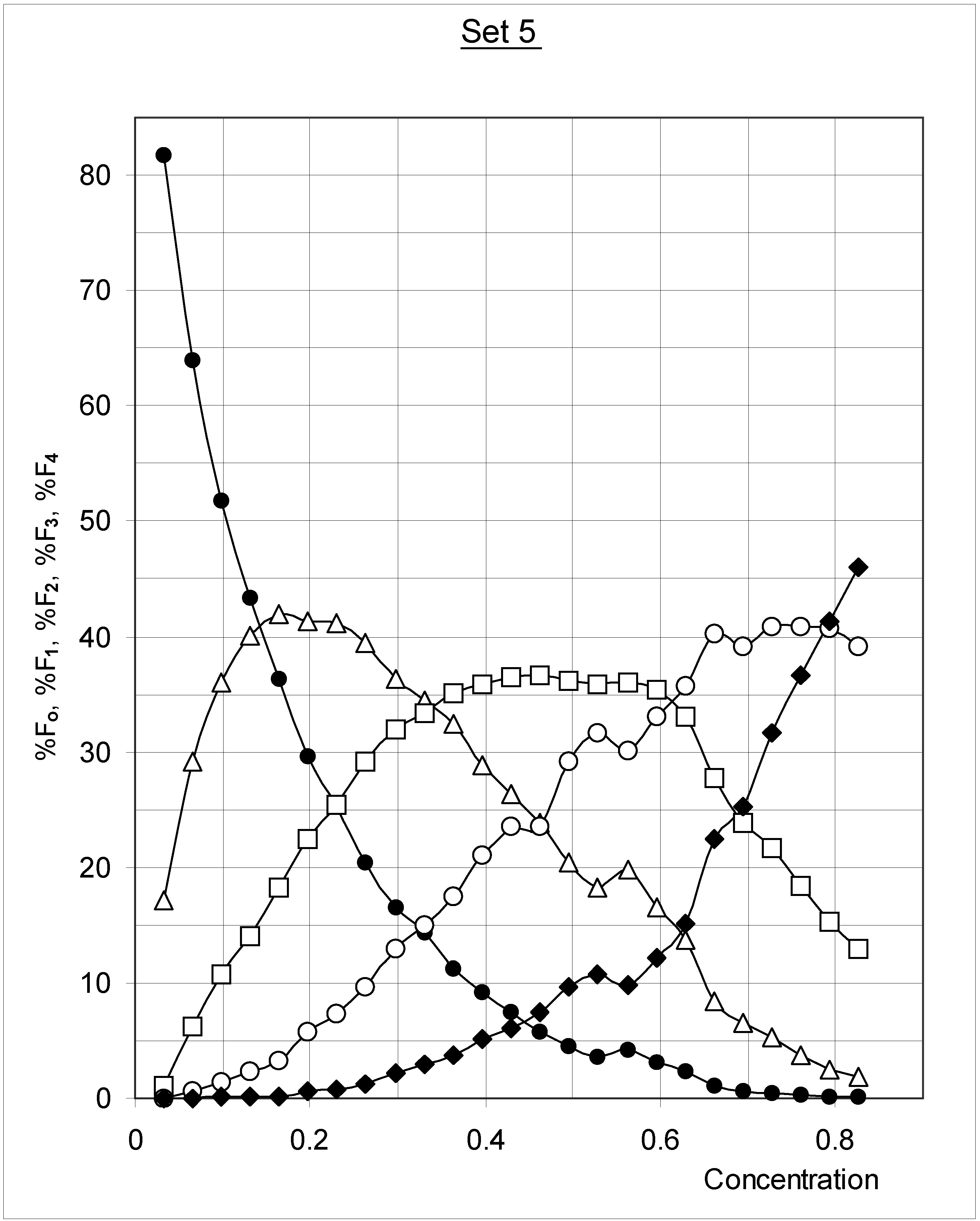
Figure 3. Variations in the distribution of occupied cells as a function of concentration for Set 5 (J = 1.5; P_B = 0.5; median inter-cell affinity). ● = %F₀; ∆ = %F₁; □ = %F₂; ○ = %F₃; ◆ = %F₄.

Figure 3. Variations in the distribution of occupied cells as a function of concentration for Set 5 (J = 1.5; P_B = 0.5; median inter-cell affinity). ● = %F₀; ∆ = %F₁; □ = %F₂; ○ = %F₃; ◆ = %F₄.

The results for Set 5 are presented in Figure 3. As concentration increased, %F₀ decreased while %F₁, %F₂, %F₃ and %F₄ increased. Then %F₁ decreased, later %F₂, and ultimately %F₃. Obviously only F₄ occupied cells would be left at a concentration of 1.00. The results for Set 3 and Set 7 are comparable, except that the maxima are shifted to lower concentrations for the higher affinity between occupied cells (Set 3), and to higher concentrations for the lower affinity (Set 7). Such a profile can be described by the compartmental model shown in Figure 4. In models of this type (which are common in chemical kinetics and pharmacokinetics), the transfer from one compartment to the other is a time-dependent process characterized by a rate constant k_i,j having the dimension of t ^–1 (t = time).

Figure 4. Compartment model used to quantify the concentration-, joining- and breaking-dependent "transfer" constants k_i,j.

Figure 4. Compartment model used to quantify the concentration-, joining- and breaking-dependent "transfer" constants k_i,j.

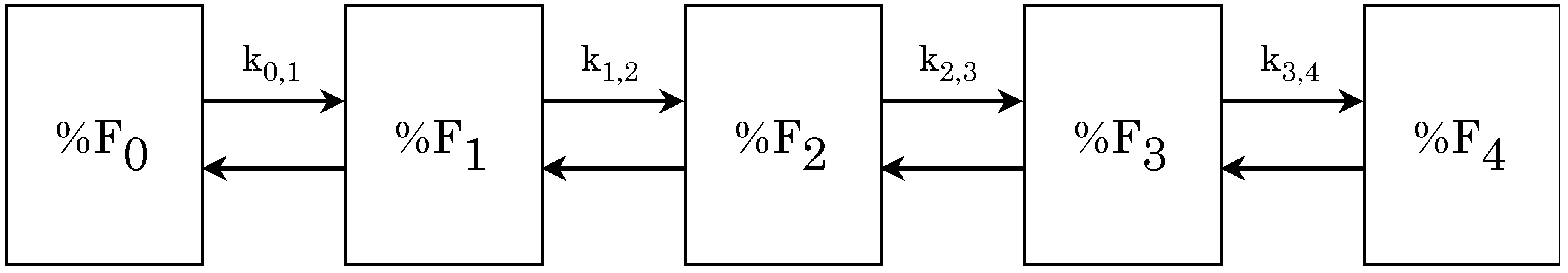
In Figure 4, the changes in %F_i in each compartment are concentration-dependent, and the "transfer" constants k_i,j will have the dimension of C⁻¹ (C = concentration). Replacing time with concentration in the common kinetic equations which describe the model in Figure 4 has yielded the following set of equations:

−d[%F₀]/d[C] = k_0,1[%F₀]

(3A)

−d[%F₁]/d[C] = k_0,1[%F₀] − k_1,2[%F₁]

(3B)

−d[%F₂]/d[C] = k_1,2[%F₁] − k_2,3[%F₂]

(3C)

−d[%F₃]/d[C] = k_2,3[%F₂] − k_3,4[%F₃]

(3D)

−d[%F₄]/d[C] = k_3,4[%F₃]

(3E)

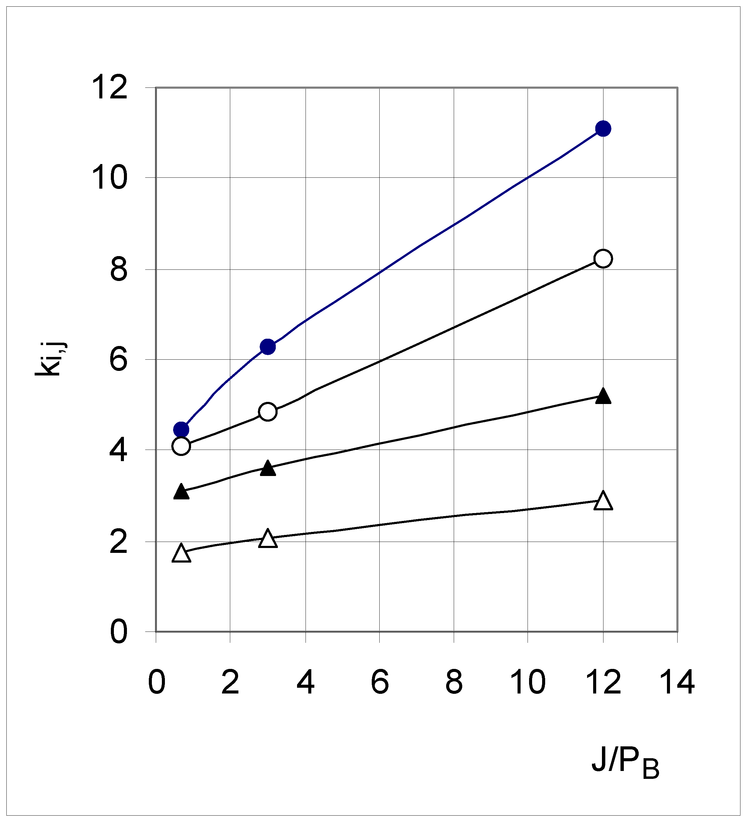
These equations were solved by the Kinetica 2.0 software for the three parameter sets, yielding the values of k_i,j shown in Table 2. For each set, the values decreased from k_0,1 to k_3,4. They also decreased from Set 3 to Set 5 to Set 7. Far from being fortuitous or random, these changes were dependent upon the joining and breaking parameters. In fact, the values of k_i,j increased with increasing joining probability, and decreased with increasing breaking probability (plots not shown). This can also be seen using an "affinity" parameter (the ratio J/P_B), with the result that k_0,1, k_1,2, k_2,3 and k_3,4 increase linearly with J/P_B (r² > 0.99) (Figure 5). Adding an indicator variable IND (with value 1, 2, 3 and 4 for k_0,1, k_1,2, k_2,3 and k_3,4, respectively) allowed the four linear equations to be merged into a single multiple linear regression equation:

k_i,j = 1.55(±0.31) J/P_B − 1.97(±0.31) IND + 4.80(±0.30)

(4A)

k_i,j = 0.581 J/P_B − 0.735 IND

(4B)

n = 12; r² = 0.879; s = 1.03; F = 32.7

which offers a fair description of Figure 5.

Table 2. Calculated "transfer" constants^a) for the compartmental model in Figure 4 and equations 3.

	Set 3	Set 5	Set 7
k0,1	11.07 ± 0.44	6.27 ± 0.11	4.47 ± 0.15
k1,2	8.23 ± 0.33	4.86 ± 0.09	4.09 ± 0.16
k2,3	5.19 ± 0.17	3.62 ± 0.08	3.10 ± 0.15
k3,4	2.91 ± 0.09	2.08 ± 0.06	1.74 ± 0.17

a) in concentration⁻¹ ± SD

Table 2. Calculated "transfer" constants^a) for the compartmental model in Figure 4 and equations 3.

	Set 3	Set 5	Set 7
k0,1	11.07 ± 0.44	6.27 ± 0.11	4.47 ± 0.15
k1,2	8.23 ± 0.33	4.86 ± 0.09	4.09 ± 0.16
k2,3	5.19 ± 0.17	3.62 ± 0.08	3.10 ± 0.15
k3,4	2.91 ± 0.09	2.08 ± 0.06	1.74 ± 0.17

a) in concentration⁻¹ ± SD

Figure 5. Influence of affinity (defined as J/P_B) on the "transfer" constants k_0,1 (●), k_1,2 (○),k_2,3 (▲) and k_3,4 (△).

Figure 5. Influence of affinity (defined as J/P_B) on the "transfer" constants k_0,1 (●), k_1,2 (○),k_2,3 (▲) and k_3,4 (△).

Conclusion of Study A

Our simulations show that in populations of particles modeled by cellular automata, the configuration of occupied cells was influenced by the concentration and the probabilities of joining and breaking. As concentration increased, occupied cells evolved toward higher configurations (F₂ , F₃ and F₄) with a kinematic-like regularity amenable to mathematical modeling. Thus, this first study succeeded in quantifying the strong influences of concentration, joining and breaking on the distribution of occupied cell configurations. In other words, correlations were found between initial conditions and one of the outputs (namely occupied cell configuration). This demonstrates and quantifies the direct constraints on occupied cell configuration (i.e., the solid arrows in Figure 1), but does not reveal indirect constraints (i.e., the broken arrows in Figure 1) which would be suggestive of additional (and unpredictable) influences of higher order.

Study B: Probability of a single occupied cell to move (%M_i)

In the second study, we followed and monitored a single occupied cell to measure its probability to move at each iteration, as influenced by its current configuration (i.e., F₀ to F₄), as well as by concentration and by the joining and breaking rules. At each iteration, the program recorded a) the configuration (F_i) of this occupied cell just before it computed its move, and b) whether it had moved or not. The monitoring of that single occupied cell was continued during 10 runs of 3000 iterations each, although preliminary tests had shown that reproducible results (i.e., 1-2% variations) were also obtained after 10 runs of 1000 or 2000 iterations each. At the end of the 30,000 iterations, the program reported the number of times the occupied cell had been in each configuration F_i (%F_i), and the number of times it had moved when in that configuration (%M_i).

Descriptive approach

The results are reported in Figure 6A, Figure 6B, Figure 6C and Figure 6D as plots of concentration versus %Mi. Since by definition F₀ occupied cells are unattached, the breaking probability does not apply and they would be expected to move at each iteration. However, it is observed in Figure 6A that a low joining inhibited the probability of an F₀ occupied cell to move and attach itself to a once-removed occupied cell (thus changing configuration). Indeed, F₀ occupied cells showed a smaller than 100% probability to move when J = 0.5 (Sets 1, 4 and 7). Furthermore, the magnitude of such an effect increased with increasing concentration. For the other joining conditions (J = 1.5 and 3.0), F₀ occupied cells moved at each iteration.

Figure 6A. Percent of moving F₀ occupied cells (%M₀) as a function of predetermined conditions. The joining probability (J) and breaking probability (P_B) are as follows: ▲ = Set 1; ∆ = Set 2; * = Set 3; ◆ = Set 4; □ = Set 5; ○ = Set 6; ■ = Set 7; ● = Set 8; ◇ = Set 9. In Figure 6A, Sets 2, 3, 5, 6, 8 and 9 have all points at 100%.

Figure 6A. Percent of moving F₀ occupied cells (%M₀) as a function of predetermined conditions. The joining probability (J) and breaking probability (P_B) are as follows: ▲ = Set 1; ∆ = Set 2; * = Set 3; ◆ = Set 4; □ = Set 5; ○ = Set 6; ■ = Set 7; ● = Set 8; ◇ = Set 9. In Figure 6A, Sets 2, 3, 5, 6, 8 and 9 have all points at 100%.

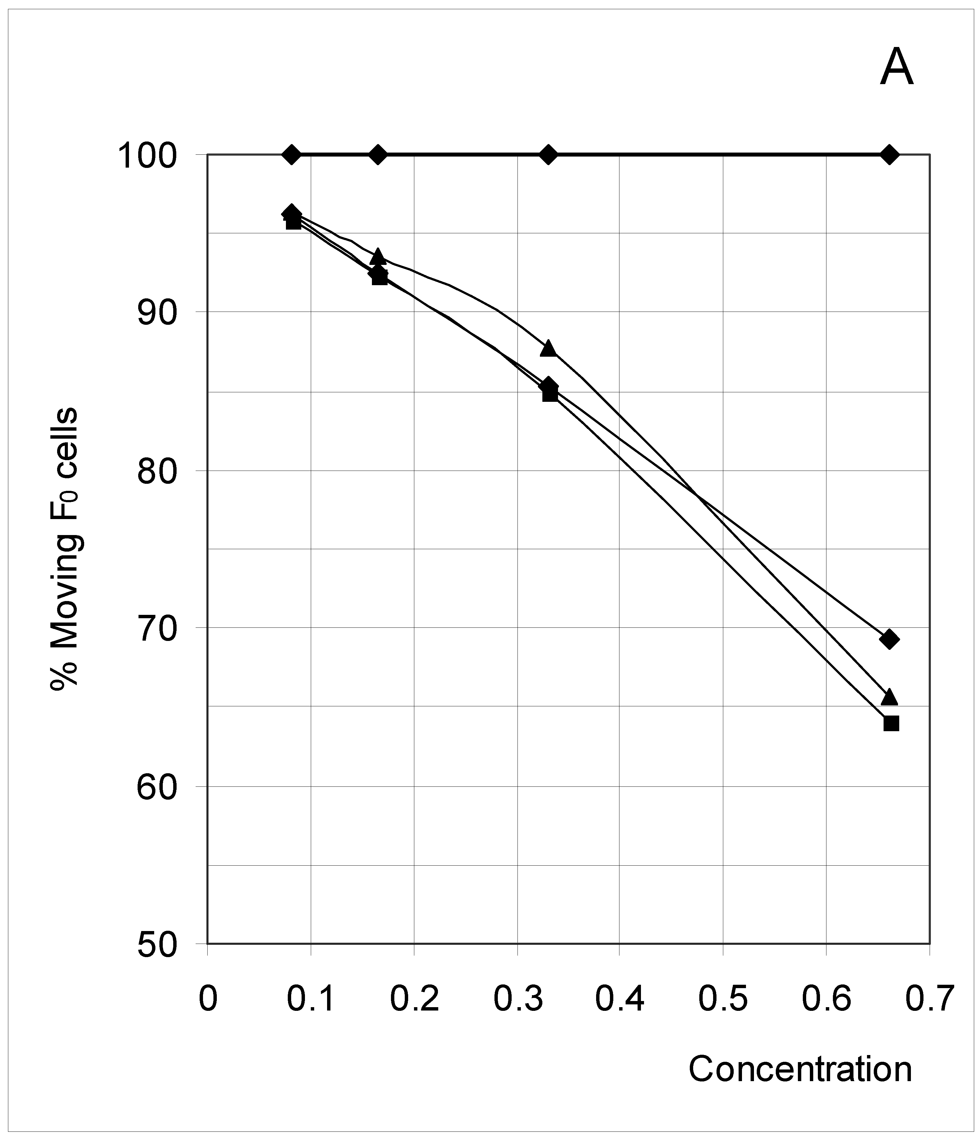
Figure 6B. Percent of moving F₁ occupied cells (%M₁) as a function of predetermined conditions. The joining probability (J) and breaking probability (P_B) are as follows: ▲ = Set 1; ∆ = Set 2; * = Set 3; ◆ = Set 4; □ = Set 5; ○ = Set 6; ■ = Set 7; ● = Set 8; ◇ = Set 9.

Figure 6B. Percent of moving F₁ occupied cells (%M₁) as a function of predetermined conditions. The joining probability (J) and breaking probability (P_B) are as follows: ▲ = Set 1; ∆ = Set 2; * = Set 3; ◆ = Set 4; □ = Set 5; ○ = Set 6; ■ = Set 7; ● = Set 8; ◇ = Set 9.

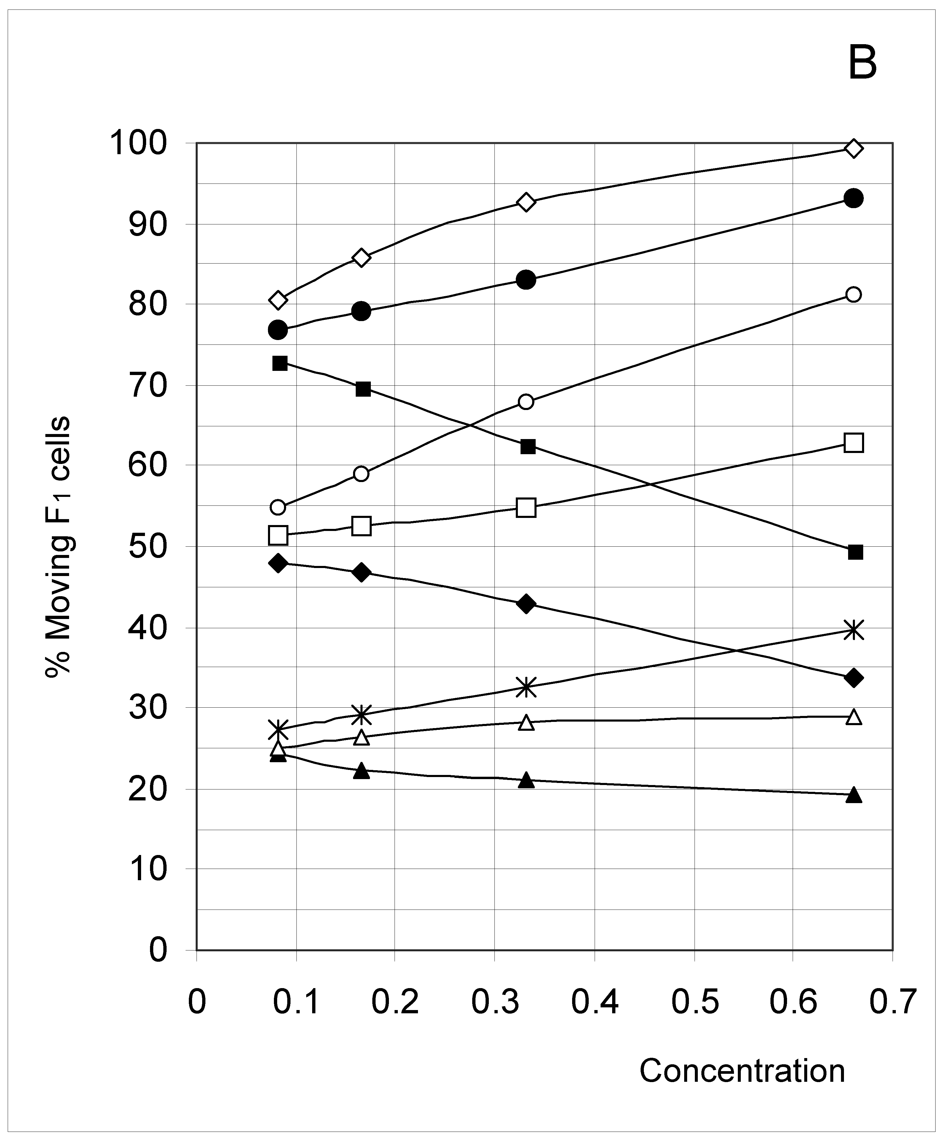
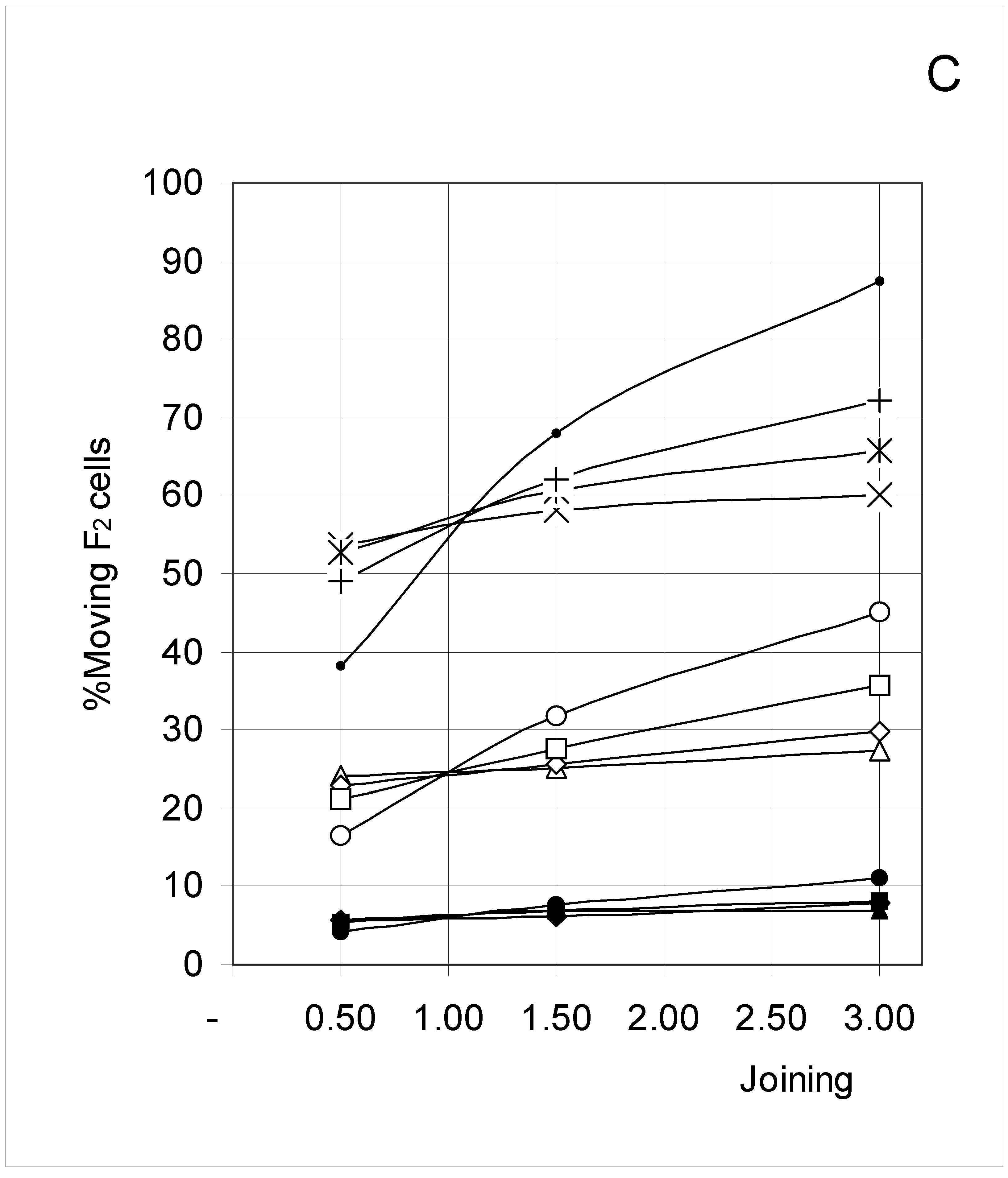
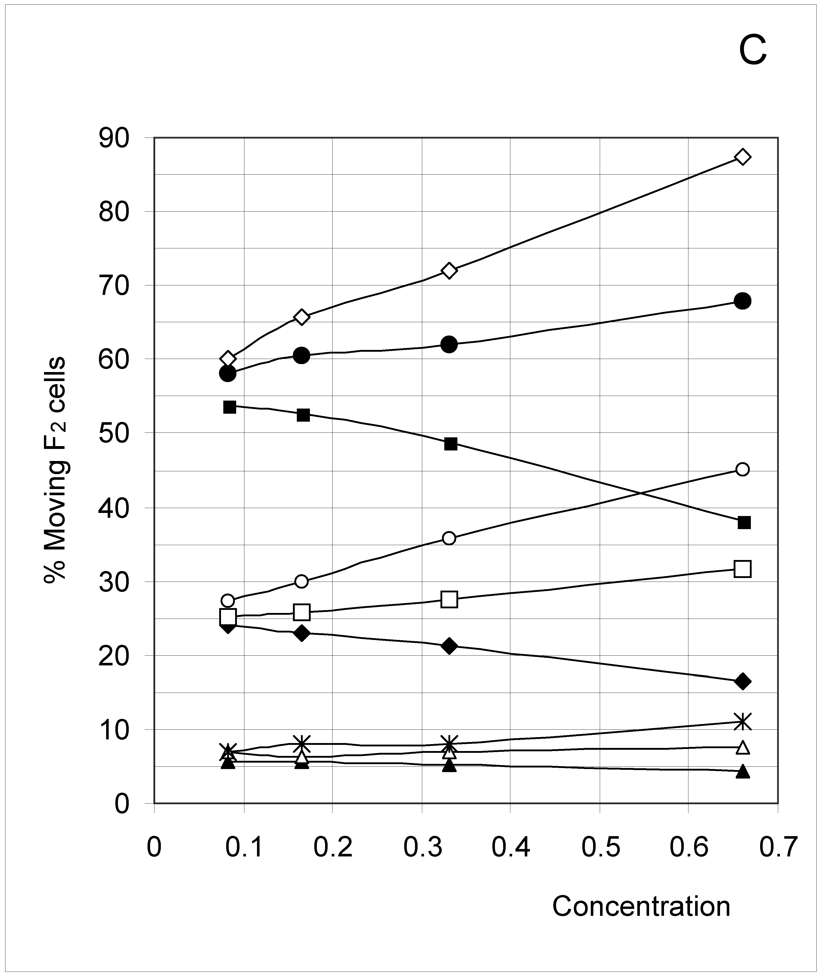
Figure 6C. Percent of moving F₂ occupied cells (%M₂) as a function of predetermined conditions. The joining probability (J) and breaking probability (P_B) are as follows: ▲ = Set 1; ∆ = Set 2; * = Set 3; ◆ = Set 4; □ = Set 5; ○ = Set 6; ■ = Set 7; ● = Set 8; ◇ = Set 9.

Figure 6C. Percent of moving F₂ occupied cells (%M₂) as a function of predetermined conditions. The joining probability (J) and breaking probability (P_B) are as follows: ▲ = Set 1; ∆ = Set 2; * = Set 3; ◆ = Set 4; □ = Set 5; ○ = Set 6; ■ = Set 7; ● = Set 8; ◇ = Set 9.

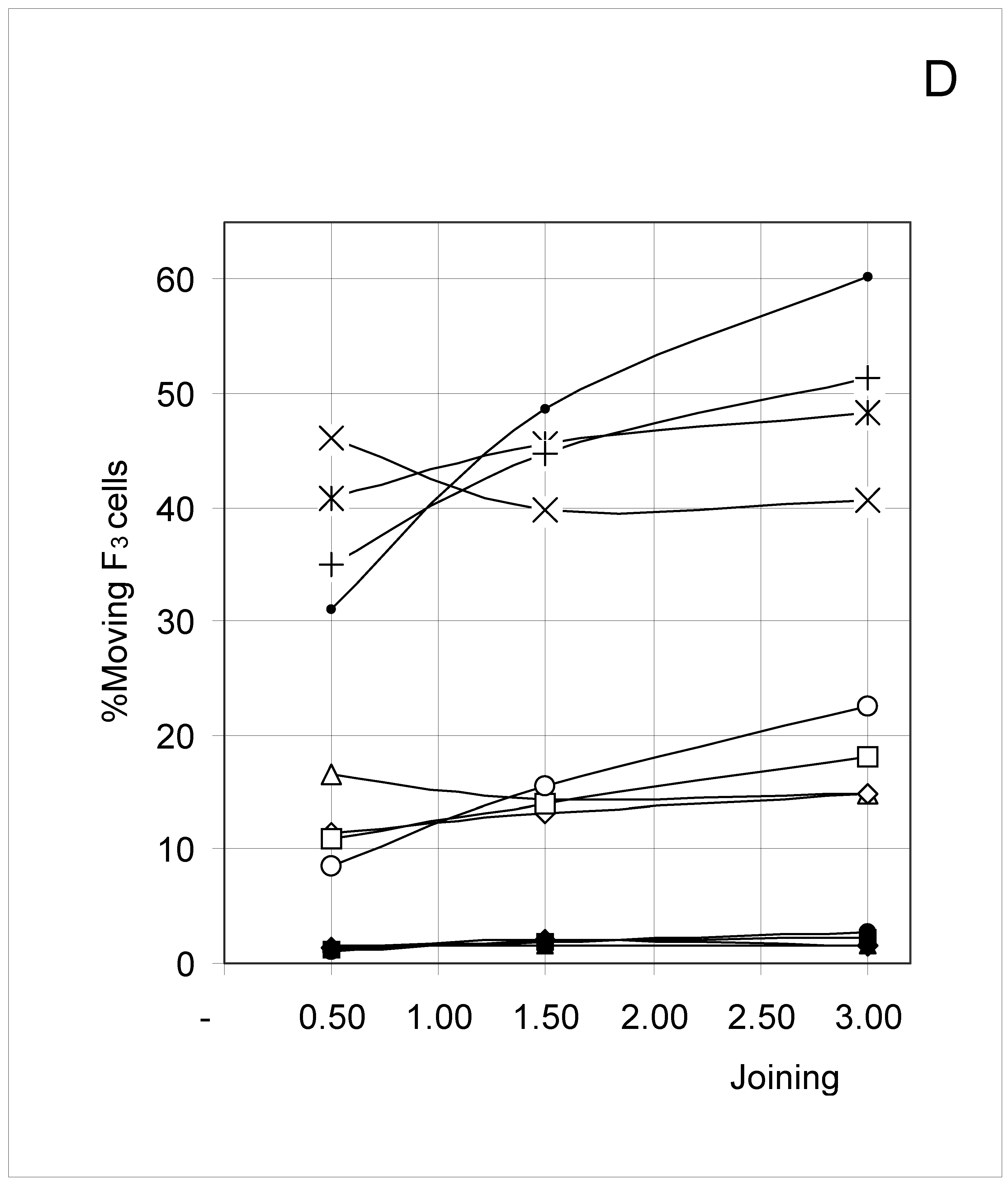
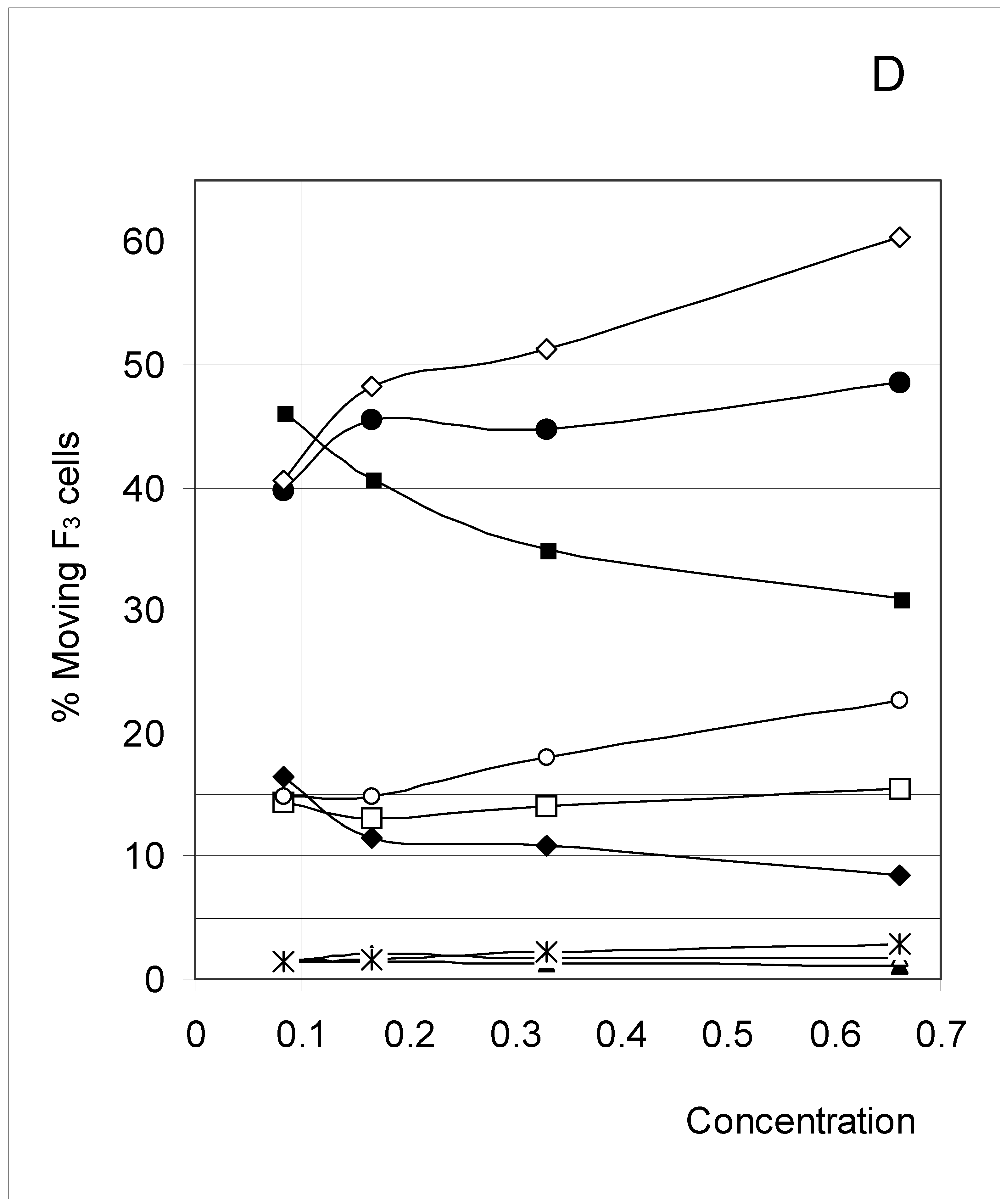
Figure 6D. Percent of moving F₃ occupied cells (%M₃) as a function of predetermined conditions. The joining probability (J) and breaking probability (P_B) are as follows: ▲ = Set 1; ∆ = Set 2; * = Set 3; ◆ = Set 4; □ = Set 5; ○ = Set 6; ■ = Set 7; ● = Set 8; ◇ = Set 9.

Figure 6D. Percent of moving F₃ occupied cells (%M₃) as a function of predetermined conditions. The joining probability (J) and breaking probability (P_B) are as follows: ▲ = Set 1; ∆ = Set 2; * = Set 3; ◆ = Set 4; □ = Set 5; ○ = Set 6; ■ = Set 7; ● = Set 8; ◇ = Set 9.

Another way to look at these results, and one in line with the major objective of this work, is to recognize that depending on its value, the joining parameter allows or forbids the concentration factor to affect the movement of F₀ occupied cells. In such a perspective, joining is seen to have a strong influence on how concentration in turn influences the movement of F₀ occupied cells. This indirect effect on the movement of F₀ occupied cells is precisely the type of unexpected constraint this study was looking for.

F₄ occupied cells cannot move, and indeed a 0% movement probability was always found. The probability of occupied cells F₁, F₂ and F₃ to move is shown in Figure 6B, Figure 6C and Figure 6D, respectively. Although the individual probabilities decreased from F₁ to F₃, the three figures show a comparable pattern. At the lower concentrations, the sets were clustered according to the breaking probability, such that Sets 1, 2 and 3 (P_B = 0.25) produced a low probability of moving, Sets 7, 8 and 9 (P_B = 0.75) a high probability of moving, and Sets 4, 5 and 6 (P_B = 0.50) an intermediate probability of moving.

As concentration increased, the influence of the joining parameter became predominant. For sets with a low joining (J = 0.5, Sets 1, 4 and 7), the probability to move decreased with increasing concentration, whereas it increased when J = 1.5 (Sets 2, 5 and 8) and mostly when J = 3.0 (Sets 3, 6 and 9). These qualitative observations indicate that joining and breaking influence the constraints imposed by concentration on the output. In other words, there is again qualitative evidence for the indirect influences we searched for. Quantitative evidence is presented in the next section.

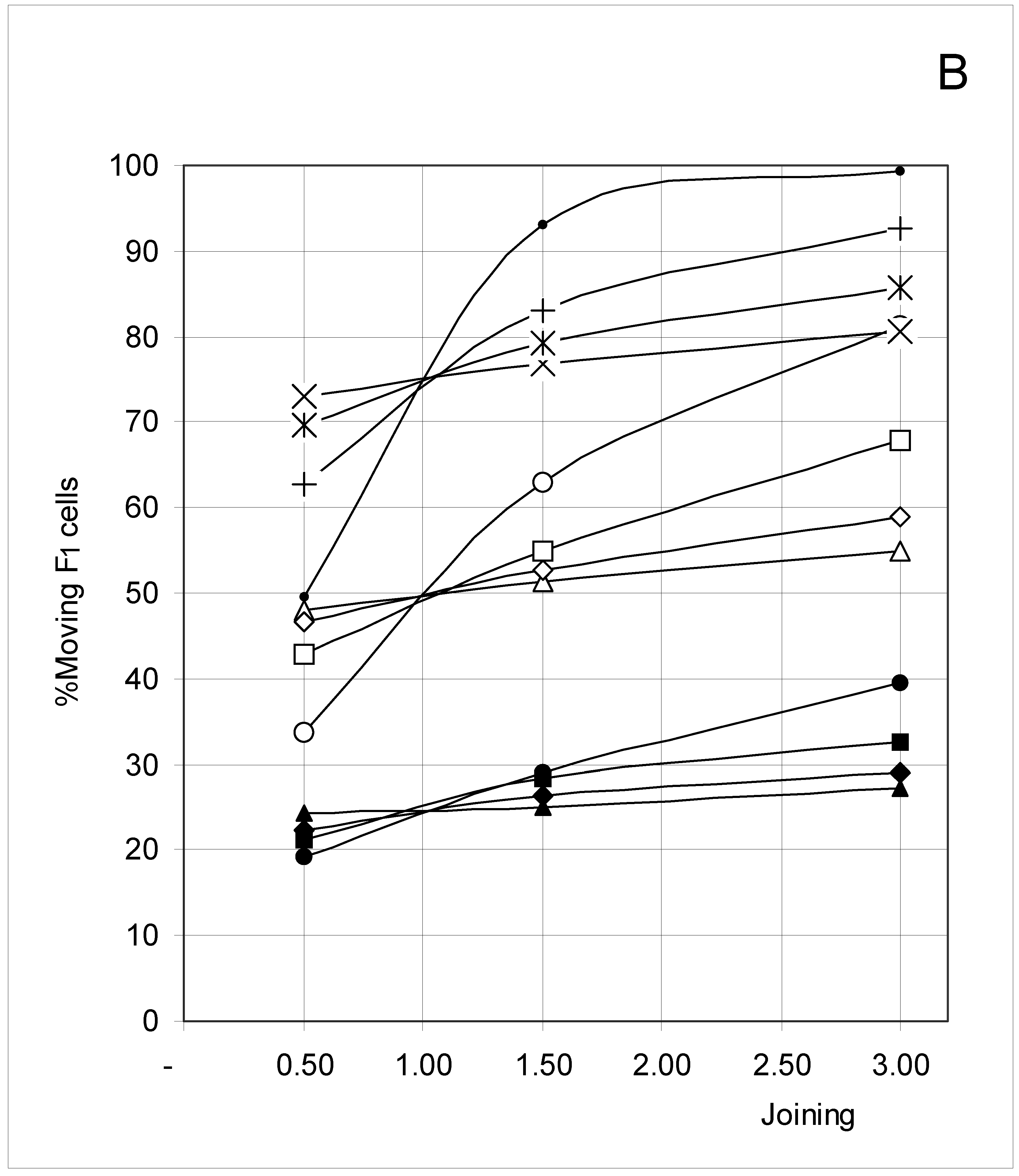
The converse indirect influence, namely that concentration influences the constraints imposed by joining and breaking, can be seen when plotting %Mi as a function of J (Figure 7A, Figure 7B, Figure 7C and Figure 7D). As a rule, %M_i increased with increasing J (see the positive slopes in Figure 7A, Figure 7B, Figure 7C and Figure 7D), with marked differences between %M₀ (Fig. 7A), %M₁ (Fig. 7B), %M₂ (Fig. 7C) and %M₃ (Fig. 7D). Significantly, these positive slopes themselves increased with increasing concentration. Indeed, the influence of joining on %M₁, %M₂ and %M₃ was practically constant at low concentrations, and strongly positive at high concentrations. But because the effects were sometimes nonlinear, no statistical analysis was performed.

Figure 7A. Percent of moving F₀ occupied cells (%M₀) as a function of predetermined conditions. The concentration (C) and breaking probability (P_B) are as follows: ▲ : C = 0.0826, P_B= 0.25; ◆ : C = 0.165, P_B= 0.25; ■ : C = 0.33, P_B= 0.25; ● : C = 0.661, P_B= 0.25; △ : C = 0.0826, P_B= 0.50; ◇ : C = 0.165, P_B= 0.50; □ : C = 0.33, P_B= 0.50; ○ : C = 0.661, P_B= 0.50; × : C = 0.0826, P_B= 0.75; * : C = 0.165, P_B= 0.75; + : C = 0.33, P_B= 0.75; • : C = 0.661, P_B= 0.75. In Figure 7A, J = 1.5 and J = 3.0 have all points at 100%.

Figure 7A. Percent of moving F₀ occupied cells (%M₀) as a function of predetermined conditions. The concentration (C) and breaking probability (P_B) are as follows: ▲ : C = 0.0826, P_B= 0.25; ◆ : C = 0.165, P_B= 0.25; ■ : C = 0.33, P_B= 0.25; ● : C = 0.661, P_B= 0.25; △ : C = 0.0826, P_B= 0.50; ◇ : C = 0.165, P_B= 0.50; □ : C = 0.33, P_B= 0.50; ○ : C = 0.661, P_B= 0.50; × : C = 0.0826, P_B= 0.75; * : C = 0.165, P_B= 0.75; + : C = 0.33, P_B= 0.75; • : C = 0.661, P_B= 0.75. In Figure 7A, J = 1.5 and J = 3.0 have all points at 100%.

Figure 7B. Percent of moving F₁ occupied cells (%M₁) as a function of predetermined conditions. The concentration (C) and breaking probability (P_B) are as follows: ▲ : C = 0.0826, P_B= 0.25; ◆ : C = 0.165, P_B= 0.25; ■ : C = 0.33, P_B= 0.25; ● : C = 0.661, P_B= 0.25; △ : C = 0.0826, P_B= 0.50; ◇ : C = 0.165, P_B= 0.50; □ : C = 0.33, P_B= 0.50; ○ : C = 0.661, P_B= 0.50; × : C = 0.0826, P_B= 0.75; * : C = 0.165, P_B= 0.75; + : C = 0.33, P_B= 0.75; • : C = 0.661, P_B= 0.75.

Figure 7B. Percent of moving F₁ occupied cells (%M₁) as a function of predetermined conditions. The concentration (C) and breaking probability (P_B) are as follows: ▲ : C = 0.0826, P_B= 0.25; ◆ : C = 0.165, P_B= 0.25; ■ : C = 0.33, P_B= 0.25; ● : C = 0.661, P_B= 0.25; △ : C = 0.0826, P_B= 0.50; ◇ : C = 0.165, P_B= 0.50; □ : C = 0.33, P_B= 0.50; ○ : C = 0.661, P_B= 0.50; × : C = 0.0826, P_B= 0.75; * : C = 0.165, P_B= 0.75; + : C = 0.33, P_B= 0.75; • : C = 0.661, P_B= 0.75.

Figure 7C. Percent of moving F₂ occupied cells (%M₂) as a function of predetermined conditions. The concentration (C) and breaking probability (P_B) are as follows: ▲ : C = 0.0826, P_B= 0.25; ◆ : C = 0.165, P_B= 0.25; ■ : C = 0.33, P_B= 0.25; ● : C = 0.661, P_B= 0.25; △ : C = 0.0826, P_B= 0.50; ◇ : C = 0.165, P_B= 0.50; □ : C = 0.33, P_B= 0.50; ○ : C = 0.661, P_B= 0.50; × : C = 0.0826, P_B= 0.75; * : C = 0.165, P_B= 0.75; + : C = 0.33, P_B= 0.75; • : C = 0.661, P_B= 0.75.

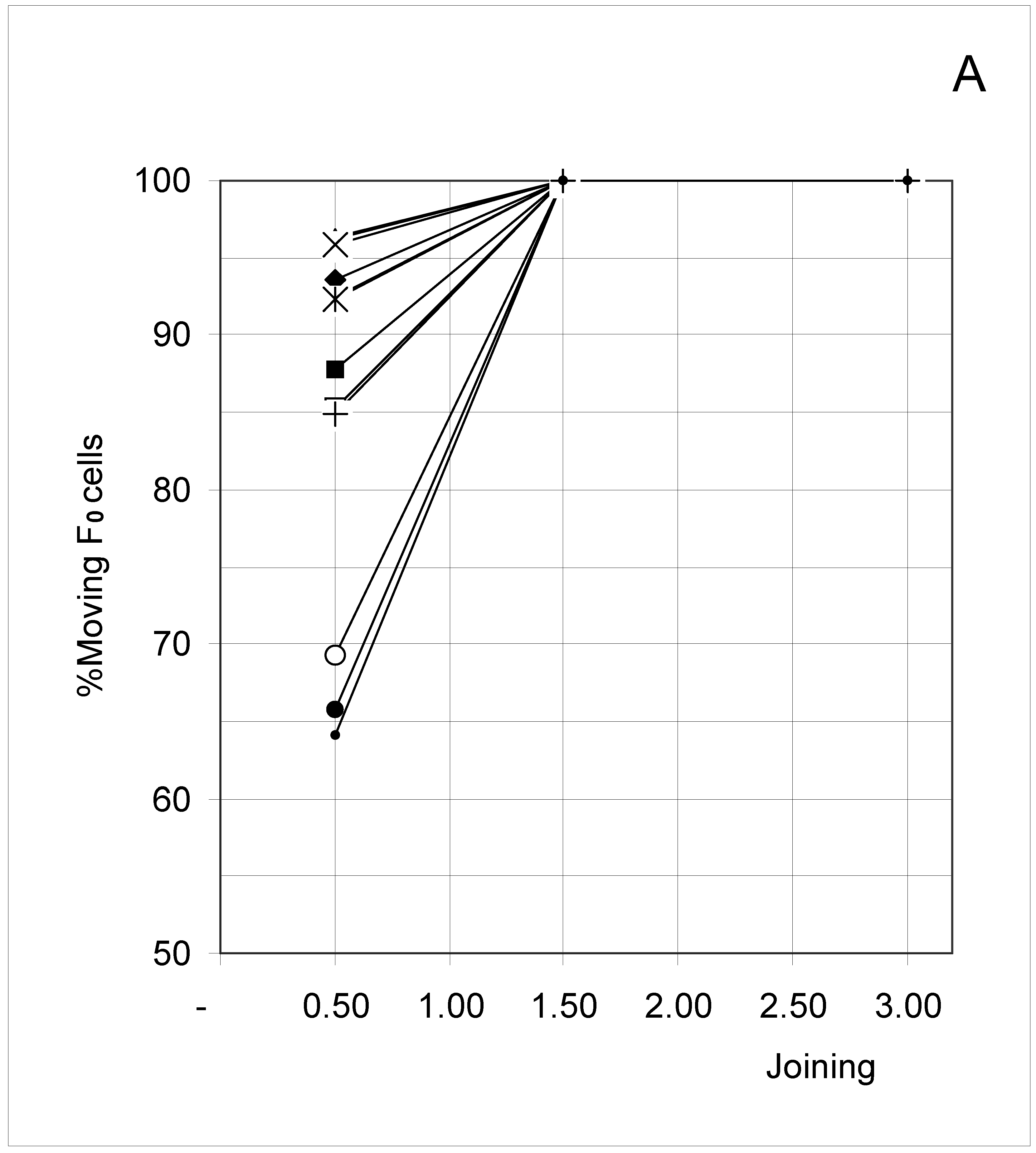
Figure 7C. Percent of moving F₂ occupied cells (%M₂) as a function of predetermined conditions. The concentration (C) and breaking probability (P_B) are as follows: ▲ : C = 0.0826, P_B= 0.25; ◆ : C = 0.165, P_B= 0.25; ■ : C = 0.33, P_B= 0.25; ● : C = 0.661, P_B= 0.25; △ : C = 0.0826, P_B= 0.50; ◇ : C = 0.165, P_B= 0.50; □ : C = 0.33, P_B= 0.50; ○ : C = 0.661, P_B= 0.50; × : C = 0.0826, P_B= 0.75; * : C = 0.165, P_B= 0.75; + : C = 0.33, P_B= 0.75; • : C = 0.661, P_B= 0.75.

Figure 7D. Percent of moving F₃ occupied cells (%M₃) as a function of predetermined conditions. The concentration (C) and breaking probability (P_B) are as follows: ▲ : C = 0.0826, P_B= 0.25; ◆ : C = 0.165, P_B= 0.25; ■ : C = 0.33, P_B= 0.25; ● : C = 0.661, P_B= 0.25; △ : C = 0.0826, P_B= 0.50; ◇ : C = 0.165, P_B= 0.50; □ : C = 0.33, P_B= 0.50; ○ : C = 0.661, P_B= 0.50; × : C = 0.0826, P_B= 0.75; * : C = 0.165, P_B= 0.75; + : C = 0.33, P_B= 0.75; • : C = 0.661, P_B= 0.75.

Figure 7D. Percent of moving F₃ occupied cells (%M₃) as a function of predetermined conditions. The concentration (C) and breaking probability (P_B) are as follows: ▲ : C = 0.0826, P_B= 0.25; ◆ : C = 0.165, P_B= 0.25; ■ : C = 0.33, P_B= 0.25; ● : C = 0.661, P_B= 0.25; △ : C = 0.0826, P_B= 0.50; ◇ : C = 0.165, P_B= 0.50; □ : C = 0.33, P_B= 0.50; ○ : C = 0.661, P_B= 0.50; × : C = 0.0826, P_B= 0.75; * : C = 0.165, P_B= 0.75; + : C = 0.33, P_B= 0.75; • : C = 0.661, P_B= 0.75.

Correlations between initial conditions and movement probability

To extract more information from the data in Figure 6A, Figure 6B, Figure 6C and Figure 6D, we looked for some quantitative relations between concentration, joining and breaking (initial conditions) and the output of the system, namely the probability of F₁, F₂ and F₃ to move as a function of concentration (Figure 6B, Figure 6C and Figure 6D).

The 36 datapoints in Figure 6B (%M₁), Figure 6C (%M₂) and Figure 6D (%M₃) were subjected to multiple linear regression analysis. Good correlations exist for all three dependent variables, accounting for more than 90% of the variance (Equations 5-7) :

%M₁ = 8.81(±5.62)C + 7.64 (±1.21) J + 103.5 (±6.1) P_B − 13.7 (±4.2)

(5A)

%M₁ = 0.082 C + 0.331 J + 0.892 P_B

(5B)

n = 36; r² = 0.912; s = 7.47; F = 110.1

%M₂ = 7.70 (±5.14) C + 5.16 (±1.11) J + 107.5 (±5.6) P_B − 32.9 (±3.9)

(6A)

%M₂ = 0.073 C + 0.225 J + 0.932 P_B

(6B)

n = 36; r² = 0.925; s = 6.84; F = 131.4

%M₃ = 2.92(±4.48) C + 2.42(±0.97) J + 85.2 (±4.9) P_B− 27.3 (±3.4)

(7A)

%M₃ = 0.035 C + 0.135 J + 0.942 P_B

(7B)

n = 36; r² = 0.907; s = 5.96; F = 104.4

Each of the three dependent variables (%M₁, %M₂ and %M₃) reveals a similar dependency, with the influence of P_B being about 3 to 7 times larger than that of J, itself 3 to 4 times larger than that of C. In contrast, the contribution of concentration was low (Eq. 5 and 6) or even non-significant (Eq. 7), because its influence was negative or positive depending on the joining parameter (negative for J = 0.5; positive for J = 1.5 and 3.0).

To quantify this effect of J on the influence of C, we analyzed the data in Figure 6B separately for J = 0.5 (Sets 1 + 4 + 7), J = 1.5 (Sets 2 + 5 + 8) and J = 3.0 (Sets 3 + 6 + 9). The same analysis was performed for the data in Figure 6C and in Figure 6D. In each case, good to very good correlations were found, with r² in the range 0.92 to 0.99. The equations for Figure 6C are shown below as an example (Eq. 8-10):

for J = 0.5 (Sets 1 + 4 + 7):

%M₂ = − 14.5(±5.3) C + 86.3(±5.8) P_B − 13.7(±3.5)

(8A)

%M₂ = − 0.176 C + 0.965 P_B

(8B)

n = 12; r² = 0.962; s = 4.09; F = 115.1

for J = 1.5 (Sets 2 + 5 + 8):

%M₂ = 9.75(±5.37) C + 110.5(±5.8) P_B − 26.0(±3.6)

(9A)

%M₂ = 0.094 C + 0.983 P_B

(9B)

n = 12; r² = 0.976; s = 4.13; F = 180.8

for J = 3.0 (Sets 3 + 6 + 9):

%M₂ = 27.8(±6.7) C + 125.6(±7.2) P_B − 33.3(±4.4)

(10A)

%M₂ = 0.231 C + 0.959 P_B

(10B)

n = 12; r² = 0.973; s = 5.12; F = 159.2

The regression coefficient of C in Eq. 8A, 9A and 10A is of particular interest, since each of its values (−14.5, 9.75 and 27.8) reflects the average slope of the 3 corresponding lines in Figure 6C. These slopes quantify the influence of C on %M₂, and they are seen to increase with J. Importantly, the relation between these slopes and J is quasi-linear (r² = 0.96; n = 3). The corresponding values for %M₁ and %M₃ are r² = 0.85 and 0.94, respectively. In other words, we have succeeded here is showing how J modifies the constraint of C on %M_i.

Conclusion of Study B

The first point to emerge from Study B is that the movement of occupied cells is conditioned by an intrinsic attribute (their configuration), by preset conditions (J and P_B), as well as by concentration. Like Study A, Study B succeeded in quantifying the strong influences of concentration, joining and breaking on one of the outputs, here the probability of occupied cells to move (%M_i). This again demonstrates and quantifies the direct constraints on cell properties (Figure 1). In essence, this first conclusion regarding an attribute of cellular automata (their freedom to move) is comparable to the conclusion of Study A regarding their configuration (F₀ to F₄).

However, the most significant result to emerge from Study B is that joining, breaking and concentration not only influence the movement of occupied cells, they also modify each other's influence on this output (Figure 1). This indirect influence is demonstrated here quite clearly, and is even quantified in one case. Such second-order constraints, not predictable from the initial conditions, have been equated with dissolvence. Their characterization has been the major objective of our CA simulations.

Relations between constraints and the emergence of percolation

In a previous study [4], we used the same setup as here to monitor the appearance of percolation, an emergent attribute of many-particle systems. When plotting concentration against the percent probability of having a dynamic percolating cluster of CA, sigmoidal curves were obtained. These allowed a C50% to be calculated, namely the concentration for which there was a 50% probability of having a percolating cluster (Table 1). Graphically (results not shown), C50% was seen to increase strongly with increasing P_B, and to decrease modestly with increasing J. Remarkably, these influences were also amenable to multiple linear regression analysis, yielding equation 11 :

C_50% = − 0.0089(±0.0018) J + 0.149(±0.009) P_B + 0.468(±0.006)

(11A)

C_50% = − 0.285 J + 0.948 P_B

(11B)

n = 9; r² = 0.980; s = 0.0055; F = 147.2

This equation is of good statistical quality and expresses in a quantitative manner the above qualitative conclusions. Of particular significance is the fact that an emergent property of the system, i.e. percolation, was dependent on joining and breaking in a manner quite similar to the constraints on movement of individual occupied cells (Eq. 5-7). Indeed, the regression coefficients of J and P_B in Eq. 11B have a ratio close to 0.30, in the same range as the corresponding ratio in Eq. 5B, 6B and 7B (0.14, 0.24 and 0.37, respectively). In other words, there is evidence here for an analogy between the conditions that govern emergence and dissolvence.

Conclusions

Expected and unexpected constraints on the behavior of CA

The first objective of this study was to examine whether and how the configurations and movements of occupied cells are determined by initial conditions. These independent variables were the concentration of occupied cells, and two predefined rules of the cellular automata simulations, namely the joining and breaking probabilities.

Figure 2, Figure 3 and Figure 5 show that the probabilistic distribution of occupied cell configurations was indeed highly dependent of concentration, joining and breaking. Figure 2A, Figure 2B, Figure 2C, Figure 2D and Figure 2E in particular describe this dependence. Quantitative descriptions were obtained by multiple linear regressions (Equations 1-4). Similar results came from monitoring the probability of movement of individual occupied cells. Here also, the influence of concentration, joining and breaking is revealed in Figure 5 and Figure 6 to be quite complex. Again, multiple linear regressions offered a partial yet informative description of the constraints experienced by individual occupied cells in the CA simulations (Equations 5-10).

When the configuration of occupied cells was the monitored output, no unexpected constraint was seen, i.e. only the full arrows in Figure 1 seemed to operate. In contrast, an unexpected fact emerged when monitoring the movement of occupied cells, namely that concentration, joining and breaking did modify each other's influence (broken arrows in Figure 1). These are indirect constraints on the individual occupied cells, not predictable from the initial conditions.

In a previous writing, some of us have reflected on the properties of sub-systems as constituents of a higher system [10,11,12]. We noted that such sub-systems experience constraints which affect their property space, options and independence [1,12,13,14]. In cellular automata, constraints on occupied cell configurations and (as monitored here for the first time) on occupied cell movement are a direct and trivial consequence of initial conditions, even if they can only be predicted qualitatively. What would be non-trivial and unpredictable, we felt, would be indirect constraints resulting from the initial conditions modifying each other's influence. Such constraints were taken as model and analogue of dissolvence in CA, and indeed they were characterized here and even quantified.

Constraints versus emergence

In a previous study, we examined the global behavior of a many-particle CA system identical to the one investigated here [4]. Specifically, we focused on an emergent property of the system, namely the formation of a percolating cluster and its probability of appearance as concentration increased. It was found that percolation appeared at higher or lower concentrations depending on the joining and breaking parameters.

In the present study, we have shown that the emergent property of percolation on the one hand, and the constraints on movement of occupied cells on the other, displayed a comparable dependence on joining and breaking. Indeed, the relative influence of the joining and breaking probabilities were comparable on the onset of percolation and on their probability to move. This analogy between the conditions that govern emergence and dissolvence may be fortuitous, or it is indicative of a deeper connection. The question remains open.

Physical relevance of the present study

Finally, the physical relevance of our many-particle CA model must be addressed. What we examined were occupied cells whose valence configuration and freedom to move depended on concentration and on rules of intercellular attraction (P_B for all its values; J when > 1) and intercellular repulsion (J when < 1). This picture bears for example resemblance with the gaseous state, and also with solutions in an inert solvent. In this analogy, occupied cells in CA are models of molecules, and the present study may be seen as a simulation of the behavior of individual molecules in a gas or an inert solvent. In other words, CA have shown here their potential to model constraints experienced by individual molecules, and to explore relations between such constraints and emergent properties of many-particle systems such as gases and solutions.

References

- Holland, J.H. Emergence - From Chaos to Order; Perseus Books: Reading, USA, 1999. [Google Scholar]
- Von Neumann, J. Theory of Self-Reproducing Automata. In Theory of Self-Reproducing Automata; Burks, A., Ed.; University of Illinois Press: Urbana, IL, 1966. [Google Scholar]
- Kier, L.B.; Cheng, C.-K.; Testa, B. Cellular automata models of biochemical phenomena. Fut. Generat. Comput. Syst. 1999, 16, 273–289. [Google Scholar] [CrossRef]
- Kier, L.B.; Cheng, C.-K.; Testa, B. A cellular automata model of the percolation process. J. Chem. Inf. Comput. Sci. 1999, 39, 326–332. [Google Scholar] [CrossRef]
- Stauffer, D. Introduction to Percolation Theory; Taylor and Francis: London, 1985. [Google Scholar]
- de Gennes, P.G. Dynamics of entangled polymer solutions II. Inclusion of hydrodynamic interaction. Macromolecules 1976, 9, 594–598. [Google Scholar] [CrossRef]
- Broadbent, S.R.; Hammersley, J.M. Percolation process (I). Crystals and mazes. Proc. Cambridge Phil. Soc. 1957, 53, 629–641. [Google Scholar] [CrossRef]
- Sahimi, M.; Gavalas, G.R.; Tsotsis, T.T. Statistical and continuum models of fluid-solid reactions in porus media. Chem. Eng. Sci. 1990, 45, 1443–1452. [Google Scholar] [CrossRef]
- Stauffer, D.; Sahimi, M. High dimensional simulation of simple immunological models. J. Theoret. Biol. 1994, 166, 289–297. [Google Scholar] [CrossRef] [PubMed]
- Testa, B.; Kier, L.B.; Carrupt, P.A. A systems approach to molecular structure, intermolecular recognition, and emergence-dissolvence in medicinal research. Med. Res. Rev. 1997, 17, 303–326. [Google Scholar] [CrossRef]
- Testa, B.; Kier, L.B. The concept of emergence-dissolvence in drug research. Adv. Drug Res. 1997, 30, 1–14. [Google Scholar]
- Testa, B.; Kier, L.B. Emergence and dissolvence in the self-organization of complex systems. Entropy 2000, 2, 1–25. Free access: http://natsci.net/reprints/entropy/2000/e2010001.pdf. [Google Scholar] [CrossRef]
- Campbell, D.T. Downward causation in hierarchically organised systems. In Studies in the Philosophy of Biology; Ayala, F.J., Dobzhansky, T., Eds.; Macmillan: London, 1974; pp. 179–186. [Google Scholar]
- Allen, T.F.H.; Hoekstra, T.W. Toward a Unified Ecology; Columbia University Press: New York, 1992; Chapter 1. [Google Scholar]
- Testa, B.; Raynaud, I.; Kier, L.B. What differentiates free amino acids and aminoacyl residues ? An exploration of conformational and lipophilicity spaces. Helv. Chim. Acta 1999, 82, 657–665. [Google Scholar] [CrossRef]
- Testa, B.; Bojarski, A. Molecules as complex adaptative systems. Constrained molecular properties and their biochemical significance. Eur. J. Pharm. Sci. 2000, 11 Suppl. 2, S2–S14. [Google Scholar] [CrossRef]
- Kier, L.B.; Cheng, C.-K. A cellular automata model of an aqueous solution. J. Chem. Inf. Comp. Sci. 1994, 34, 1334–1337. [Google Scholar] [CrossRef]
- Kier, L.B.; Cheng, C.-K.; Testa, B.; Carrupt, P.A. A cellular automata model of the hydrophobic effect. Pharm. Res. 1995, 12, 615–619. [Google Scholar] [CrossRef] [PubMed]
- Kier, L.B.; Cheng, C.-K.; Testa, B.; Carrupt, P.A. A cellular automata model of micelle formation. Pharm. Res. 1996, 13, 1419–1422. [Google Scholar] [CrossRef] [PubMed]
- Kier, L.B.; Cheng, C.-K.; Testa, B.; Carrupt, P.A. A cellular automata model of aqueous diffusion. J. Pharm. Sci. 1997, 87, 774–778. [Google Scholar] [CrossRef] [PubMed]
- Kier, L.B.; Cheng, C.-K.; Tute, M.; Seybold, P.G. A cellular automata model of acid dissociation. J. Chem. Inf. Comp. Sci. 1998, 38, 271–275. [Google Scholar] [CrossRef]
- Steppan, D.; Werner, J.; Yeater, B. Essential Regression and Experimental Design, version 2.218; 1998. http://www.geocities.com/SiliconValley/Network/1021/.
© 2001 by MDPI. All rights reserved.
Share and Cite
MDPI and ACS Style
Testa, B.; Kier, L.B.; Cheng, C.-K.; Mayer, J. A Cellular Automata Study of Constraints (Dissolvence) in a Percolating Many-Particle System. Entropy 2001, 3, 27-57. https://doi.org/10.3390/e3020027
AMA Style
Testa B, Kier LB, Cheng C-K, Mayer J. A Cellular Automata Study of Constraints (Dissolvence) in a Percolating Many-Particle System. Entropy. 2001; 3(2):27-57. https://doi.org/10.3390/e3020027
Chicago/Turabian StyleTesta, Bernard, Lemont B. Kier, Chun-Kao Cheng, and Joachim Mayer. 2001. "A Cellular Automata Study of Constraints (Dissolvence) in a Percolating Many-Particle System" Entropy 3, no. 2: 27-57. https://doi.org/10.3390/e3020027