A New Thermodynamics from Nuclei to Stars

Abstract

Equilibrium statistics of Hamiltonian systems is correctly described by the microcanonical ensemble. Classically this is the manifold of all points in the N−body phase space with the given total energy. Due to Boltzmann’s principle, e^S = tr(δ(E − H)), its geometrical size is related to the entropy S(E, N, ⋯). This definition does not invoke any information theory, no thermodynamic limit, no extensivity, and no homogeneity assumption, as are needed in conventional (canonical) thermo-statistics. Therefore, it describes the equilibrium statistics of extensive as well of non-extensive systems. Due to this fact it is the fundamental definition of any classical equilibrium statistics. It can address nuclei and astrophysical objects as well. All kind of phase transitions can be distinguished sharply and uniquely for even small systems. It is further shown that the second law is a natural consequence of the statistical nature of thermodynamics which describes all systems with the same – redundant – set of few control parameters simultaneously. It has nothing to do with the thermodynamic limit. It even works in systems which are by far larger than any thermodynamic ”limit”.

1 Introduction

Classical thermodynamics and the theory of phase transitions of homogeneous and large systems are some of the oldest and best established theories in physics. It may look strange to add anything new to it. Let me recapitulate what was told to us since > 100 years and still told today c.f.[1]:

• thermodynamics addresses large homogeneous systems at equilibrium (in the thermodynamic limit N → ∞|_{N/V = ρ,homogeneous}).
• Phase transitions are the positive zeros of the grand-canonical partition sum Z(T, µ, V ) as function of e^βµ (Yang-Lee-singularities). As the partition sum for a finite number of particles is always positive, zeros can only exist in the thermodynamic limit V|_β,µ → ∞.
• Micro and canonical ensembles are equivalent. 1
• thermodynamics works with intensive variables T, P, µ.
• Unique Legendre mapping T → E.
• Heat only flows from hot to cold (Clausius)
• Second law only in infinite systems when the Poincarré recurrence time becomes infinite (much larger than the age of the universe (Boltzmann)).

Under these constraint only a tiny part of the real world of equilibrium systems can be treated. The ubiquitous non-homogeneous systems: nuclei, clusters, polymers, soft matter (biological) systems, but also the largest, astrophysical systems are not covered. Even normal systems with short-range coupling at phase separations are non-homogeneous and can only be treated within conventional homogeneous thermodynamics (e.g. van-der-Waals theory) by bridging the unstable region of negative compressibility by an artificial Maxwell construction. Thus even the original goal, for which thermodynamics was invented some 150 years ago, the description of steam engines is only artificially solved. There is no (grand-)canonical ensemble of phase separated and, consequently, non-homogeneous, configurations. It has a deep reason as I will discuss below: here the systems have a negative heat capacity C (resp. susceptibility). This, however, is impossible in the (grand-)canonical theory where C ∝ (δE)²

In this paper I will describe a generalization which takes Boltzmann’s principle serious and avoids the thermodynamic limit. This opens thermodynamics to the much larger world of nonextensive systems. The most prominent example are of course self-gravitating astrophysical systems which I will discuss here also. All the so familiar paradigms above have an only limited validity and are clearly violated at the most interesting situations as shown below.

Moreover, it helps to clarify the physical background of the statistical approach: The incom-pleteness of our knowledge of the degrees of freedom leads to the various ensembles and to their characteristic differences. Thermodynamics describes the properties of the entire ensemble not of a specific system (point in phase-space). Further, it will clarify the importance and origin of the fluctuations. It will shed new light on the microscopic mechanism leading to first order phase transitions. Finally, it will illuminate the origin of irreversibility and the second law out of the time-reversible microscopic equations of motion.

2 Boltzmann’s principle

The Microcanonical ensemble is the ensemble (manifold) of all possible points in the 6N dimensional phase space at the prescribed sharp energy E:

$$W\left(E,N,V\right)={є}_{0}tr\delta \left(E-H_N\right)$$

(4)

$$tr\delta \left(E-H_N\right)={\displaystyle \int \frac{d^{3N}p d^{3N}q}{N!{\left(2\pi \hslash \right)}^{3N}}}\delta \left(E-H_N\right).$$

(5)

thermodynamics addresses the whole ensemble. It is ruled by the topology of the geometrical size W (E, N, ⋯), Boltzmann’s principle:

(6)

is the most fundamental definition of the entropy S. Entropy and with it micro-canonical thermodynamics has therefore a pure mechanical, geometrical foundation. No information theoretical formulation is needed. Moreover, in contrast to the canonical entropy, S(E, N, ..) is everywhere single valued and multiple differentiable. There is no need for extensivity, no need of concavity, no need of additivity, and no need of the thermodynamic limit. This is a great advantage of the geometric foundation of equilibrium statistics over the conventional definition by the Boltzmann-Gibbs canonical theory. However, addressing entropy to finite eventually small systems we will face a new problem with Zermelo’s objection against the monotonic rise of entropy, the second law, when the system approaches its equilibrium. This is discussed in section (5) c.f.[2, 3]. A further comment: In contrast to many authors like Schrödinger [4] our ensemble is not an ensemble of non-interacting replica of the considered system which may exchange energy. I do not consider the different ways to distribute energy over the different replica. I consider the manifold of the same system at the precisely given energy under all possible different distributions of the momenta and positions of its constituents (particles) in the 6N-dimensional phase space. The result is then the average behaviour when one does not know the precise position and momentum of every particle but only the total energy.

3 Topological properties of S(E, ⋯)

The topology of the Hessian of S(E, ⋯), the determinant of curvature of s(e, n) determines completely all kinds phase transitions. This is evidently so, because e^S(E)−E/T is the weight of each energy in the canonical partition sum at given T, see footnote 1. Consequently, at phase separation this has at least two maxima, the two phases. And in between two maxima there must be a minimum where the curvature of S(E) is positive. I.e. the positive curvature detects phase separation. This is also in the case of several conserved control parameters.

$$\begin{array}{ccc}d\left(e,n\right)& =& \Vert \begin{array}{cc}\frac{{\partial }^{2}s}{\partial e^2}& \frac{{\partial }^{2}s}{\partial n\partial e}\\ \frac{{\partial }^{2}s}{\partial n\partial e}& \frac{{\partial }^{2}s}{\partial n^2}\end{array}\Vert ={\lambda }_1{\lambda }_2\\ {\lambda }_1& \ge & {\lambda }_2\to \text{eigenvectors}:\hspace{1em}{v}_1,v_2\end{array}$$

(7)

Of course for a finite system each of these maxima of S(E, ⋯) − E/T have a non-vanishing width. There are intrinsic fluctuations in each phase.

3.1 Unambiguous signal of phase transitions in a ”Small” system [5]

The whole zoo of phase-transitions can be sharply seen and distinguished. This is here demonstrated for the Potts-gas model on a two dimensional lattice of finite size of 50 × 50 lattice points, c.f. fig.(1)

3.2 Systematic of phase transitions in the micro-canonical ensemble without invoking the thermodynamic limit

• A single stable phase of course with some intrinsic fluctuations (width) by a negative largest curvature λ₁ < 0. Here s(e, n) is concave (downwards bending) in both directions. Then there is a one to one mapping of the canonical ↔the micro-ensemble.
• A transition of first order with phase separation and surface tension is indicated by λ₁(e, n) > 0. s(e, n) has a convex intruder (upwards bending) in the direction v₁ of the largest curvature ≥ 0 which can be identified with the order parameter [7]. Three solutions of

  $$\beta =\frac{1}{T}={\frac{\partial S}{\partial E}|}_s$$

  $$v=\frac{\mu }{T}=-{\frac{\partial S}{\partial N}|}_s$$

  determine the intensive temperature T = 1/β and the chemical potential Tν.
  In the thermodynamic limit the whole region {o₁, o₃} is mapped into a single point in the canonical ensemble which is consequently non-local in o. I.e. if the curvature of S(E, N ) is λ₁ ≥ 0 both ensembles are not equivalent even in the limit.
• A continuous (“second order”) transition with vanishing surface tension, where two neighboring phases become indistinguishable. This is indicated in figure (1) by a line with λ₁ = 0 and extremum of λ₁ in the direction of order parameter v_λ=0 · ∇λ₁ = 0. These are the catastrophes of the Laplace transform E → T .

3.3 CURVATURE

We saw that the curvature (Hessian) of S(E, N, ⋯) controls the phase transitions. What is the physics behind the curvature? For short-range force it is linked to the interphase surface tension.

Table 1. Parameters of the liquid–gas transition of small sodium clusters (MMMC-calculation [7]) in comparison with the bulk for a rising number N₀ of atoms, N_surf is the average number of surface atoms (estimated here as ${\displaystyle \sum N_{cluster}^{2/3}}$) of all clusters with N_i ≥ 2 together. σ/T_tr = ∆s_surf ∗ N₀/N_surf corresponds to the surface tension. Its bulk value is adjusted to agree with the experimental values of the a_s parameter which we used in the liquid-drop formula for the binding energies of small clusters, c.f. Brechignac et al. [8], and which are used in this calculation [7] for the individual clusters.

	N0	200	1000	3000	bulk
Na	Ttr [K]	940	990	1095	1156
	qlat [eV ]	0.82	0.91	0.94	0.923
	sboil	10.1	10.7	9.9	9.267
	∆ssurf	0.55	0.56	0.44
	Nsurf	39.94	98.53	186.6	∞
	σ/Ttr	2.75	5.68	7.07	7.41

Table 1. Parameters of the liquid–gas transition of small sodium clusters (MMMC-calculation [7]) in comparison with the bulk for a rising number N₀ of atoms, N_surf is the average number of surface atoms (estimated here as ${\displaystyle \sum N_{cluster}^{2/3}}$) of all clusters with N_i ≥ 2 together. σ/T_tr = ∆s_surf ∗ N₀/N_surf corresponds to the surface tension. Its bulk value is adjusted to agree with the experimental values of the a_s parameter which we used in the liquid-drop formula for the binding energies of small clusters, c.f. Brechignac et al. [8], and which are used in this calculation [7] for the individual clusters.

	N0	200	1000	3000	bulk
Na	Ttr [K]	940	990	1095	1156
	qlat [eV ]	0.82	0.91	0.94	0.923
	sboil	10.1	10.7	9.9	9.267
	∆ssurf	0.55	0.56	0.44
	Nsurf	39.94	98.53	186.6	∞
	σ/Ttr	2.75	5.68	7.07	7.41

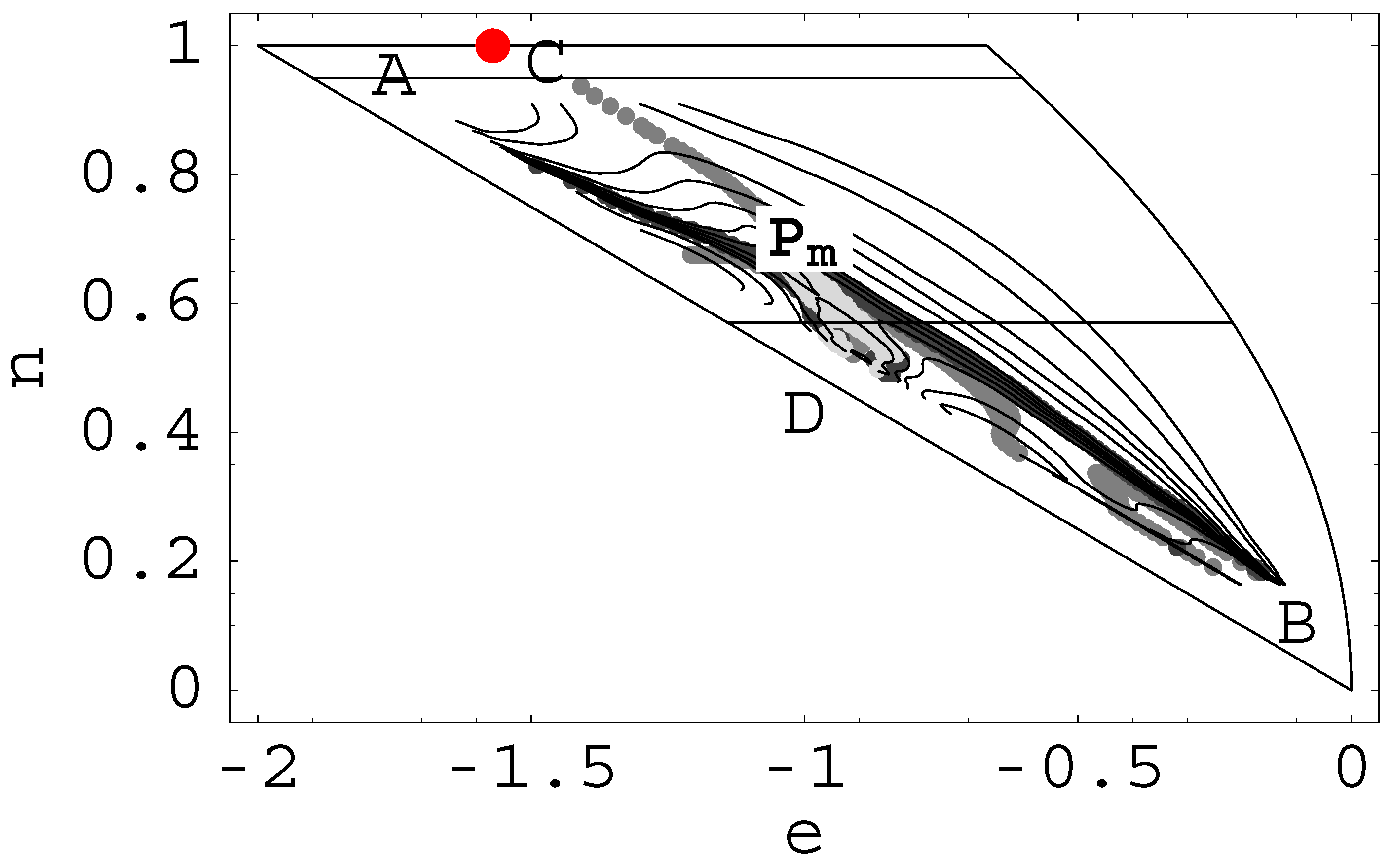
Figure 1. Global phase diagram or contour plot of the curvature determinant (Hessian), eqn. (7), of the 2-dim Potts-3 lattice gas with 50 ∗ 50 lattice points, n is the number of particles per lattice point, e is the total energy per lattice point. The line (-2,1) to (0,0) is the ground-state energy of the lattice-gas as function of n. The most right curve is the locus of configurations with completely random spin-orientations (maximum entropy). The whole physics of the model plays between these two boundaries. At the dark-gray lines the Hessian is det = 0,this is the boundary of the region of phase separation (the triangle AP_mB) with a negative Hessian (λ₁ > 0, λ₂ < 0). Here, we have Pseudo-Riemannian geometry. At the light-gray lines is a minimum of det(e, n) in the direction of the largest curvature (v_λmax · ∇det = 0) and det = 0,these are lines of second order transition. In the triangle AP_mC is the pure ordered (solid) phase (det > 0, λ₁ < 0). Above and right of the line CP_mB is the pure disordered (gas) phase (det > 0, λ₁ < 0). The crossing P_m of the boundary lines is a multi-critical point. It is also the critical end-point of the region of phase separation (det < 0, λ₁ > 0, λ₂ < 0). The light-gray region around the multi-critical point P_m corresponds to a flat, horizontal region of det(e, n) ∼ 0 and consequently to a somewhat extended cylindrical region of s(e, n) and ∇λ₁∼ 0, details see [6, 7]; C is the analytically known position of the critical point which the ordinary q = 3 Potts model (without vacancies) would have in the thermodynamic limit

Figure 1. Global phase diagram or contour plot of the curvature determinant (Hessian), eqn. (7), of the 2-dim Potts-3 lattice gas with 50 ∗ 50 lattice points, n is the number of particles per lattice point, e is the total energy per lattice point. The line (-2,1) to (0,0) is the ground-state energy of the lattice-gas as function of n. The most right curve is the locus of configurations with completely random spin-orientations (maximum entropy). The whole physics of the model plays between these two boundaries. At the dark-gray lines the Hessian is det = 0,this is the boundary of the region of phase separation (the triangle AP_mB) with a negative Hessian (λ₁ > 0, λ₂ < 0). Here, we have Pseudo-Riemannian geometry. At the light-gray lines is a minimum of det(e, n) in the direction of the largest curvature (v_λmax · ∇det = 0) and det = 0,these are lines of second order transition. In the triangle AP_mC is the pure ordered (solid) phase (det > 0, λ₁ < 0). Above and right of the line CP_mB is the pure disordered (gas) phase (det > 0, λ₁ < 0). The crossing P_m of the boundary lines is a multi-critical point. It is also the critical end-point of the region of phase separation (det < 0, λ₁ > 0, λ₂ < 0). The light-gray region around the multi-critical point P_m corresponds to a flat, horizontal region of det(e, n) ∼ 0 and consequently to a somewhat extended cylindrical region of s(e, n) and ∇λ₁∼ 0, details see [6, 7]; C is the analytically known position of the critical point which the ordinary q = 3 Potts model (without vacancies) would have in the thermodynamic limit

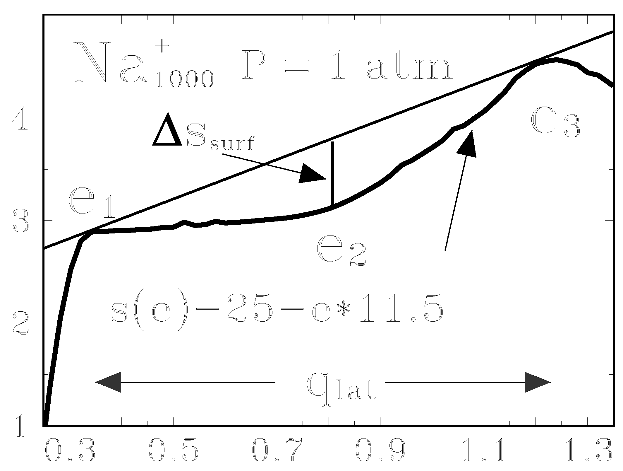
Figure 2. MMMC [7] simulation of the entropy s(e) per atom (e in eV per atom) of a system of N₀ = 1000 sodium atoms at an external pressure of 1 atm. At the energy e ≤ e₁ the system is in the pure liquid phase and at e ≥ e₃ in the pure gas phase, of course with fluctuations. The latent heat per atom is q_lat = e₃ − e₁. Attention: the curve s(e) is artificially sheared by subtracting a linear function 25 + e∗11.5 in order to make the convex intruder visible. s(e) is always a steep monotonic rising function. We clearly see the global concave (downwards bending) nature of s(e) and its convex intruder. Its depth is the entropy loss due to additional correlations by the interfaces. It scales ∝ N^−1/3 . From this one can calculate the surface tension per surface atom σ_surf/T_tr = ∆s_surf ∗ N₀/N_surf. The double tangent (Gibbs construction) is the concave hull of s(e). Its derivative gives the Maxwell line in the caloric curve T(e) at T_tr. In the thermodynamic limit the intruder would disappear and s(e) would approach the double tangent from below. Nevertheless, even there, the probability ∝ e^Ns of configurations with phase-separations are suppressed by the (infinitesimal small) factor $e^{-N^{2/3}}$ relative to the pure phases and the distribution remains strictly bimodalin the canonical ensemble. The region e₁ < e < e₃ of phase separation gets lost.

Figure 2. MMMC [7] simulation of the entropy s(e) per atom (e in eV per atom) of a system of N₀ = 1000 sodium atoms at an external pressure of 1 atm. At the energy e ≤ e₁ the system is in the pure liquid phase and at e ≥ e₃ in the pure gas phase, of course with fluctuations. The latent heat per atom is q_lat = e₃ − e₁. Attention: the curve s(e) is artificially sheared by subtracting a linear function 25 + e∗11.5 in order to make the convex intruder visible. s(e) is always a steep monotonic rising function. We clearly see the global concave (downwards bending) nature of s(e) and its convex intruder. Its depth is the entropy loss due to additional correlations by the interfaces. It scales ∝ N^−1/3 . From this one can calculate the surface tension per surface atom σ_surf/T_tr = ∆s_surf ∗ N₀/N_surf. The double tangent (Gibbs construction) is the concave hull of s(e). Its derivative gives the Maxwell line in the caloric curve T(e) at T_tr. In the thermodynamic limit the intruder would disappear and s(e) would approach the double tangent from below. Nevertheless, even there, the probability ∝ e^Ns of configurations with phase-separations are suppressed by the (infinitesimal small) factor $e^{-N^{2/3}}$ relative to the pure phases and the distribution remains strictly bimodalin the canonical ensemble. The region e₁ < e < e₃ of phase separation gets lost.

3.4 Heat can flow from cold to hot

In figure (3) it is shown how a convexity of s(e) leads to a violation of Clausius’ first formulation of the second law.

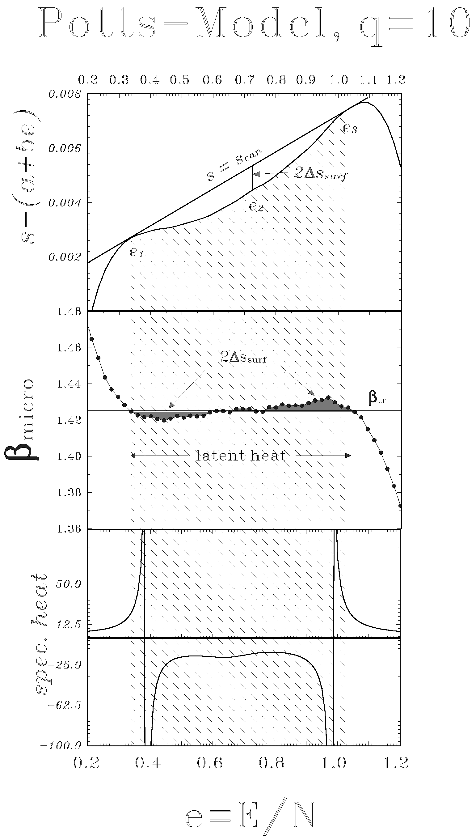
Figure 3. Potts model, (q = 10) in the region of phase separation. At e₁ the system is in the pure ordered phase, at e₃ in the pure disordered phase. A little above e₁ the temperature T = 1/β is higher than a little below e₃. Combining two parts of the system: one at the energy e₁ + δe and at the temperature T₁, the other at the energy e₃ − δe and at the temperature T₃< T₁ will equilibrize with a rise of its entropy, a drop of T₁ (cooling) and an energy flow (heat) from 3 → 1: i.e.: Heat flows from cold to hot! Clausius formulation of the second law is violated. Evidently, this is not any peculiarity of gravitating systems! This is a generic situation within classical thermodynamics even of systems with short-range coupling and has nothing to do with long range interaction.

Figure 3. Potts model, (q = 10) in the region of phase separation. At e₁ the system is in the pure ordered phase, at e₃ in the pure disordered phase. A little above e₁ the temperature T = 1/β is higher than a little below e₃. Combining two parts of the system: one at the energy e₁ + δe and at the temperature T₁, the other at the energy e₃ − δe and at the temperature T₃< T₁ will equilibrize with a rise of its entropy, a drop of T₁ (cooling) and an energy flow (heat) from 3 → 1: i.e.: Heat flows from cold to hot! Clausius formulation of the second law is violated. Evidently, this is not any peculiarity of gravitating systems! This is a generic situation within classical thermodynamics even of systems with short-range coupling and has nothing to do with long range interaction.

4 Negative heat capacity as signal for a phase transition of first order.

In the previous discussion we saw the phenomenon of first-order phase-transitions is linked to the appearance of non-homogeneities at phase-separations, and inter-phase surfaces. This, then gives rise to the convexity of S(order-parameter and the appearance of negative susceptibilities (e.g. a negative heat capacity). These are ubiquitous in nature from the smallest to the largest systems:

4.1 Nuclear Physics

A very detailed illustration of the appearance of negative heat capacities is given by D’Agostino et al. [9]. Here I want to remember one of the oldest experimental finding of a ”back”-bending caloric curve in Nuclear Physics.

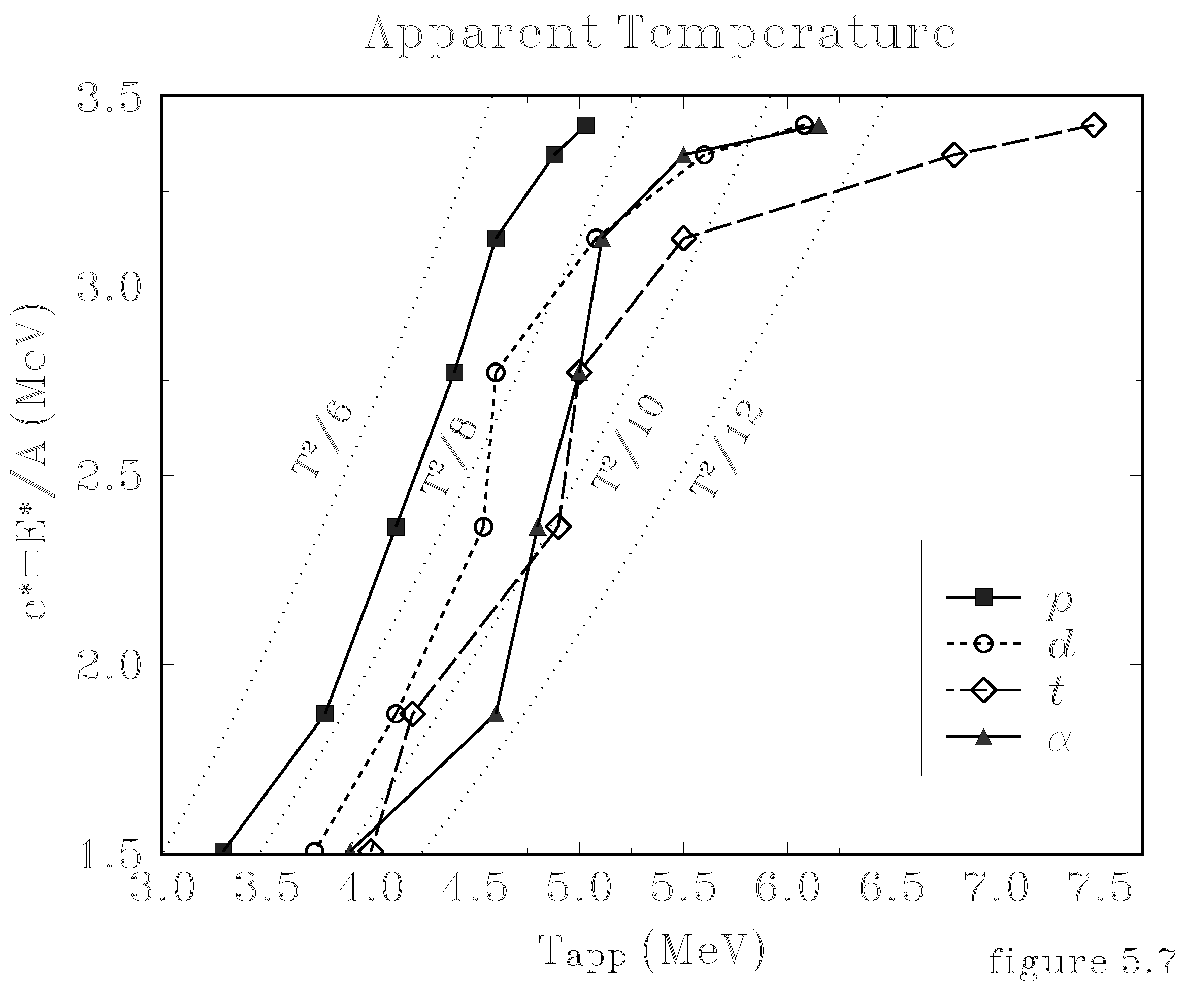
Figure 4. Experimental excitation energy per nucleon e* versus apparent temperature T_app for backward p, d, t and α together with heavy evaporation residues out of incomplete fusion of 701 Mev ²⁸Si+¹⁰⁰Mo. The dotted curves give the Fermi-gas caloric curves for the level-density parameter a = 6 to 12. (Chbihi et al. Eur.Phys.J. A 1999)

Figure 4. Experimental excitation energy per nucleon e* versus apparent temperature T_app for backward p, d, t and α together with heavy evaporation residues out of incomplete fusion of 701 Mev ²⁸Si+¹⁰⁰Mo. The dotted curves give the Fermi-gas caloric curves for the level-density parameter a = 6 to 12. (Chbihi et al. Eur.Phys.J. A 1999)

4.2 Atomic clusters

Here I show the simulation of a typical fragmentation transition of a system of 3000 sodium atoms interacting by realistic (many-body) forces. To compare with usual macroscopic conditions, the calculations were done at each energy using a volume V (E) such that the microcanonical pressure $P=\frac{\partial S}{\partial V}/\frac{\partial S}{\partial E}=1\text{atm}$. The inserts above give the mass distribution at the various points. The label ”4:1.295” means 1.295 quadrimers on average. This gives a detailed insight into what happens with rising excitation energy over the transition region: At the beginning (e* ∼ 0.442 eV) the liquid sodium drop evaporates 329 single atoms and 7.876 dimers and 1.295 quadrimers on average. At energies e >∼ 1eV the drop starts to fragment into several small droplets (”intermediate mass fragments”) e.g. at point 3: 2726 monomers,80 dimers,∼10 trimers, ∼30 quadrimers and a few heavier ones up to 10-mers. The evaporation residue disappears. This multifragmentation finishes at point 4. It induces the strong backward swing of the caloric curve T (E). Above point 4 one has a gas of free monomers and at the beginning a few dimers. This transition scenario has a lot similarity with nuclear multifragmentation. It is also shown how the total interphase surface area, proportional to $N_{eff}^{2/3}={\displaystyle {\sum }_i{N}_i^{2/3}}$ with N_i ≥ 2 (N_i the number of atoms in the ith cluster) stays roughly constant up to point 3 even though the number of fragments ($N_{fr}={\sum }_i$) is monotonic rising with increasing excitation.

Figure 5. Cluster fragmentation

Figure 5. Cluster fragmentation

4.3 Stars

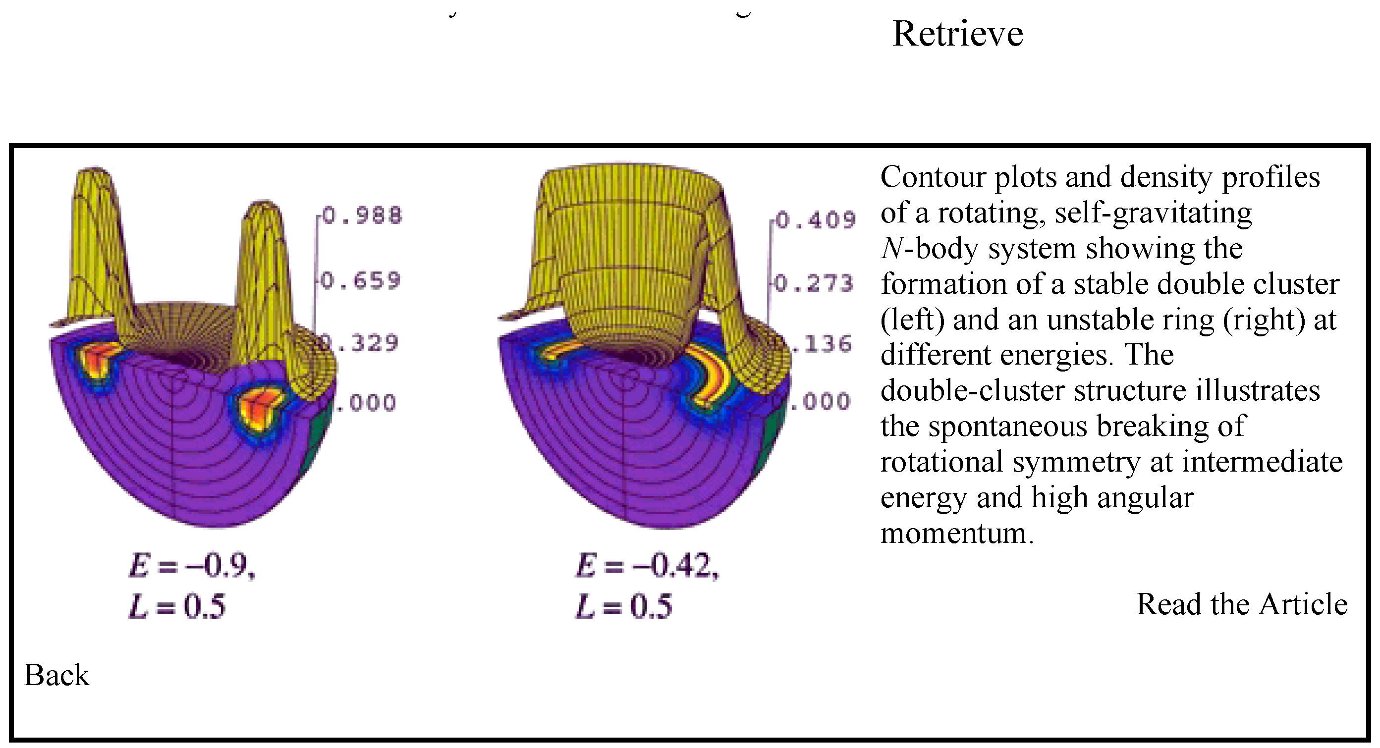
Self-gravitation leads to a non-extensive potential energy ∝ N². No thermodynamic limit exists for E/N and no canonical treatment makes sense. At negative total energies these systems have a negative heat capacity. This was for a long time considered as an absurd situation within canonical statistical mechanics with its thermodynamic “limit”. However, within our geometric theory this is just a simple example of the pseudo-Riemannian topology of the microcanonical entropy S(E, N) provided that high densities with their non-gravitational physics, like nuclear hydrogen burning, are excluded. We treated the various phases of a self-gravitating cloud of particles as function of the total energy and angular momentum, c.f. the quoted paper. Clearly these are the most important constraint in astrophysics.

Figure 6. Phases and Phase-Separation in Rotating, Self-Gravitating Systems, Physical Review Letters–July 15, 2002, cover-page, by (Votyakov, Hidmi, De Martino, Gross)

Figure 6. Phases and Phase-Separation in Rotating, Self-Gravitating Systems, Physical Review Letters–July 15, 2002, cover-page, by (Votyakov, Hidmi, De Martino, Gross)

5 The second law, microcanonically

There are many attempts to derive the second law of thermodynamics from Statistical Mechanics e.g. by Einstein or recently by Lieb and many others [10, 11, 12, 13]. Lebowitz gave an excellent and deep discussion of the present day understanding of irreversibility [14, 15, 1]. His “Statistical mechanics: A selective review of two central issues” addresses exactly to the two issues I want to discuss here. They are closely related but there are also deep differences as will become evident in the following.

In this paper I want to emphasize an important aspect of statistical mechanics of many-body systems which to my opinion was not sufficiently considered up to now: Statistical Mechanics and with it also thermodynamics are macroscopic theories describing the average behaviour of all many-body systems with the same but redundant macroscopic constraint and information. This fact leads in a simple and straight forward manner to the desired understanding of irreversibility and the second law for systems obeying a time reversible microscopic dynamics. It is important to deduce the second law from reversible (here Newtonian) and not from dissipative dynamics as is often done because just the derivation of irreversibility from fully reversible dynamics is the main challenge.

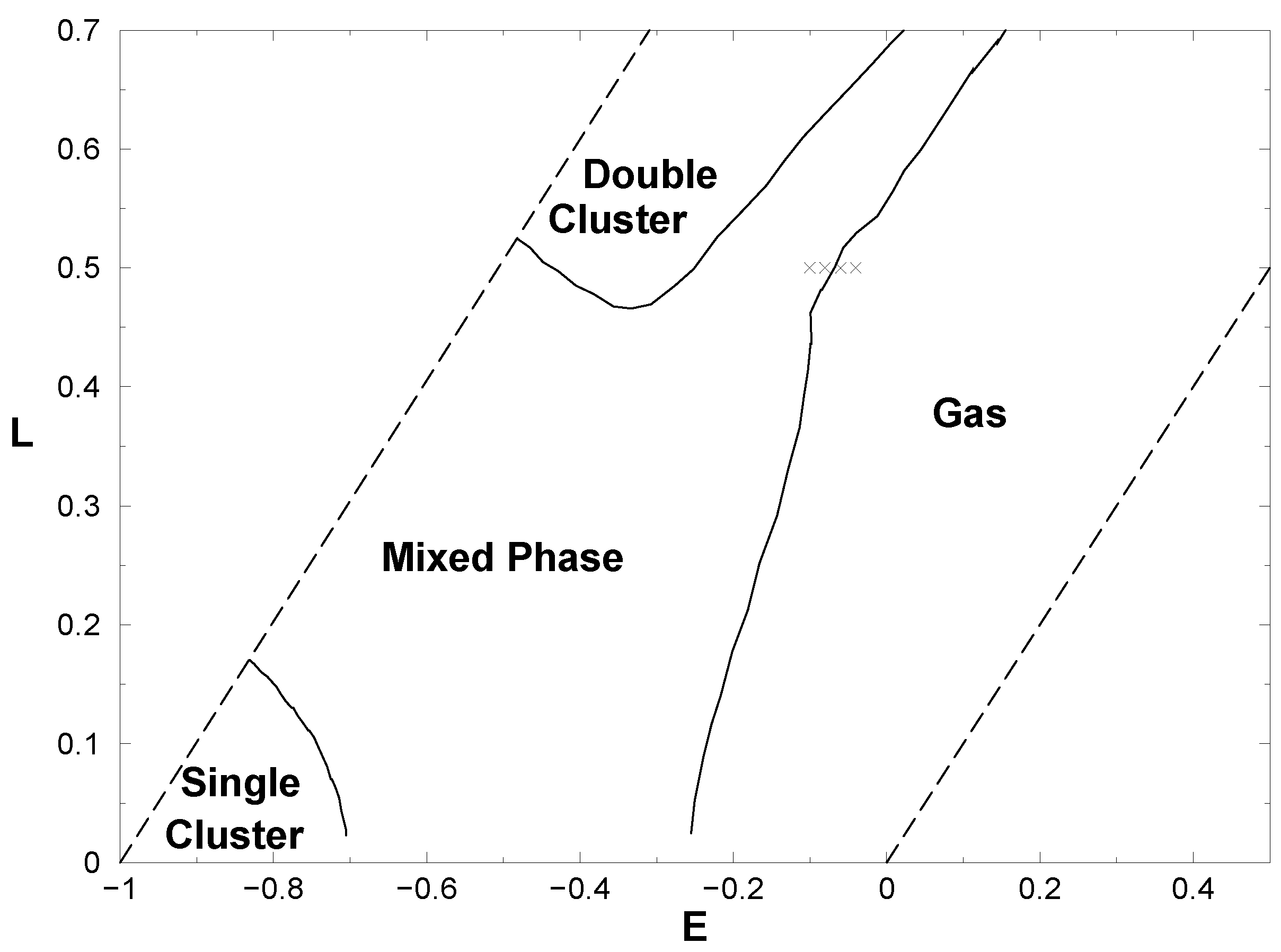
Figure 7. Microcanonical phase-diagram of a cloud of self-gravitating and rotating system as function of the energy and angular-momentum. Outside the dashed boundaries only some singular points were calculated. In the mixed phase the largest curvature λ₁ of S(E, L) is positive. Consequently the heat capacity or the correspondent susceptibility is negative. This is of course well known in astrophysics. However, the new and important point of our finding is that within microcanonical thermodynamics this is a generic property of all phase transitions of first order, independently of whether there is a short- or a long-range force that organizes the system.

Figure 7. Microcanonical phase-diagram of a cloud of self-gravitating and rotating system as function of the energy and angular-momentum. Outside the dashed boundaries only some singular points were calculated. In the mixed phase the largest curvature λ₁ of S(E, L) is positive. Consequently the heat capacity or the correspondent susceptibility is negative. This is of course well known in astrophysics. However, the new and important point of our finding is that within microcanonical thermodynamics this is a generic property of all phase transitions of first order, independently of whether there is a short- or a long-range force that organizes the system.

The new approach that I will present here was derived from the experience that Gibbs’ canonical statistics fails to describe properly the large and important group of non-extensive systems. These are systems subjected to an interaction with a range comparable to or larger than their linear dimension. They are strongly non-homogeneous and are either finite and have a surface, or they show a strong clustering like astrophysical objects, or they are split spatially in regions of different structures (phases) like a system at the liquid-gas phase separation.

5.1 Measuring a macroscopic observable, the “ EPS-formulation ”

A single point {q_i(t), p_i(t)}_i=1⋯N in the N-body phase space corresponds to a detailed specification of the system with all degrees of freedom (d.o.f) completely fixed at time t (microscopic determination). Fixing only the total energy E of an N-body system leaves the other (6N − 1)-degrees of freedom unspecified. A second system with the same energy is most likely not in the same microscopic state as the first, it will be at another point in phase space, the other d.o.f. will be different. I.e. the measurement of the total energy ${\widehat{H}}_N$, or any other macroscopic observable $\widehat{M}$, determines a (6N − 1)-dimensional sub-manifold $\mathcal{E}$ or $\mathcal{M}$ in phase space2. (The manifold $\mathcal{M}$ is called by Lebowitz a macrostate[14, 15, 1] which contains Γ_M = W (M ) microstates.) All points (the microstates) in N-body phase space consistent with the given value of E and volume V, i.e. all points in the (6N − 1)-dimensional sub-manifold $\mathcal{E}\left(N,V\right)$ of phase space are equally consistent with this measurement. $\mathcal{E}\left(N,V\right)$is the microcanonical ensemble. This example tells us that any macroscopic measurement is incomplete and defines a sub-manifold of points in phase space not a single point. An additional measurement of another macroscopic quantity $\widehat{B}\left\{q,p\right\}$ reduces $\mathcal{E}$ further to the cross-section $\mathcal{E}\cap \mathcal{B}$, a (6N − 2)-dimensional subset of points in $\mathcal{E}$ with the volume:

$$W\left(B,E,N,V\right)=\frac{1}{N!}{{\displaystyle \int \left(\frac{d^{3}q{d}^{3}p}{{\left(2\pi \hslash \right)}^3}\right)}}^N{є}_0\delta (E-{\widehat{H}}_N\{q,p\})\delta (B-\widehat{B}\{q,p\})$$

(8)

If ${\widehat{H}}_N\left\{q,p\right\}$ as also $\widehat{B}\left\{q,p\right\}$ are continuous differentiable functions of their arguments, what we assume in the following, $\mathcal{E}\cap \mathcal{B}$ is closed. In the following we use W for the Riemann or Liouville volume of a many-fold.

Microcanonical thermostatics gives the probability P (B, E, N, V ) to find the N-body system in the sub-manifold $\mathcal{E}\cap \mathcal{B}$(E, N, V ):

$$P\left(B,E,N,V\right)=\frac{W\left(B,E,N,V\right)}{W\left(E,N,V\right)}=e^{\ln \left[W\left(B,E,N,V\right)\right]-S\left(E,N,V\right)}$$

(9)

This is what Krylov seems to have had in mind [16] and what I will call the “ensemble probabilistic formulation of statistical mechanics (EPS) ”.

Similarly thermodynamics describes the development of some macroscopic observable $\widehat{B}\left\{q_t,p_t\right\}$ in time of systems which were specified at an earlier time t₀ by another macroscopic measurement $\widehat{A}\left\{q_0,p_0\right\}$. It is related to the volume of the sub-manifold $\mathcal{M}\left(t\right)=\mathcal{A}\left(t_0\right)\cap \mathcal{B}\left(t\right)\cap \mathcal{E}$:

$$W\left(A,B,E,t\right)=\frac{1}{N!}{\displaystyle \int {\left(\frac{d^3{q}_t d^3{p}_t}{{\left(2\pi \hslash \right)}^3}\right)}^N}\delta \left(B-\widehat{B}\left\{q_t,p_t\right\}\right)\delta \left(A-\widehat{A}\left\{q_0,p_0\right\}\right){є}_0\delta \left(E-\widehat{H}\left\{q_t,p_t\right\}\right),$$

(10)

where {q_t{q₀, p₀}, p_t{q₀, p₀}} is the set of trajectories solving the Hamilton-Jacobi equations

$${\dot{q}}_t=\frac{\partial \widehat{H}}{\partial p_i}, {\dot{p}}_t=-\frac{\partial \widehat{H}}{\partial q_i}, i=1\cdots N$$

(11)

with the initial conditions {q(t = t₀) = q₀; p(t = t₀) = p₀}. For a very large system with N ∼ 10²³ the probability to find a given value B(t), P(B(t)), is usually sharply peaked as function of B. Ordinary thermodynamics treats systems in the thermodynamic limit N → ∞ and gives only < B(t) >. However, here we are interested to formulate the second law for “Small” systems i.e. we are interested in the whole distribution P (B(t)) not only in its mean value < B(t) >. thermodynamics does not describe the temporal development of a single system (single point in the 6N-dim phase space).

There is an important property of macroscopic measurements: Whereas the macroscopic constraint $\widehat{A}\left\{q_0,p_0\right\}$ determines (usually) a compact region $\mathcal{A}\left(t_0\right)$ in {q₀, p₀} this does not need to be the case at later times t ≫ t₀: $\mathcal{A}\left(t\right)$ defined by $\mathcal{A}\left\{q_0\left\{q_t,p_t\right\},p_0\left\{q_t,p_t\right\}\right\}$ might become a fractal i.e. “spaghetti-like” manifold as a function of {q_t, p_t} in $\mathcal{E}$ at t → ∞ and loose compactness.

This can be expressed in mathematical terms: There exist series of points $\left\{a_n\right\}\in \mathcal{A}\left(t\right)$ which converge to a point a_∞ which is not in $\mathcal{A}\left(t\right)$. E.g. such points a_∞ may have intruded from the phase space complimentary to $\mathcal{A}\left(t_0\right)$. Illustrative examples for this evolution of an initially compact submanifold into a fractal set are the baker transformation discussed in this context by ref. [17, 18]. Then no macroscopic (incomplete) measurement at late time t can resolve a_∞ from its immediate neighbors a_n in phase space with distances |a_n − a_∞| less then any arbitrary small δ. In other words, at the time t ≫ t₀ no macroscopic measurement with its incomplete information about {q_t, p_t} can decide whether $\left\{q_0\left\{q_t,p_t\right\},p_0\left\{q_t,p_t\right\}\right\}\in \mathcal{A}\left(t_0\right)$ or not. I.e. any macroscopic theory like thermodynamics can only deal with the closure of $\mathcal{A}\left(t\right)$. If necessary, the sub-manifold $\mathcal{A}\left(t\right)$ must be artificially closed to $\overline{\mathcal{A}}\left(t\right)$ as developed further in section 5.2. Clearly, in this approach this is the physical origin of irreversibility.

5.2 Fractal distributions in phase space, second law

Here we will first describe a simple working-scheme (i.e. a sufficient method) which allows to deduce mathematically the second law. Later, we will show how this method is necessarily implied by the reduced information obtainable by macroscopic measurements.

Let us examine the following Gedanken experiment: Suppose the probability to find our system at points ${\left\{q_t,p_t\right\}}_1^N$ in phase space is uniformly distributed for times t < t₀ over the sub-manifold $\mathcal{E}\left(N,V_1\right)$ of the N-body phase space at energy E and spatial volume V₁. At time t > t₀ we allow the system to spread over the larger volume V₂ > V₁ without changing its energy. If the system is dynamically mixing, the majority of trajectories ${\left\{q_t,p_t\right\}}_1^N$ in phase space starting from points {q₀, p₀} with q₀ ⊂ V₁ at t₀ will now spread over the larger volume V₂. Of course the Liouvillean measure of the distribution $\mathcal{M}\left\{q_t,p_t\right\}$ in phase space at t > t₀ will remain the same $\left(=tr\left[\mathcal{E}\left(N,V_1\right)\right]\right)$ [19]. (The label {q₀ ⊂ V₁} of the integral means that the positions ${\left\{q_0\right\}}_1^N$ are restricted to the volume V₁, the momenta ${\left\{p_0\right\}}_1^N$ are unrestricted.)

$$\begin{array}{ccc}\hfill tr\left[\mathcal{M}\left\{q_t\left\{q_0,p_0\right\},p_t\left\{q_0,p_0\right\}\right\}\right]{|}_{\left\{q_0\subset V_1\right\}}& =& {{\displaystyle {\int }_{\left\{q_0\left\{q_t,p_t\right\}\subset V_1\right\}}\frac{1}{N!}\left(\frac{d^3{q}_t d^3{p}_t}{{\left(2\pi \hslash \right)}^3}\right)}}^N{є}_0\delta \left(E-{\widehat{H}}_N\left\{q_t,p_t\right\}\right)\hfill \\ & =& {{\displaystyle {\int }_{\left\{q_0\subset V_1\right\}}\frac{1}{N!}\left(\frac{d^3{q}_0 d^3{p}_0}{{\left(2\pi \hslash \right)}^3}\right)}}^N{є}_0\delta \left(E-{\widehat{H}}_N\left\{q_0,p_0\right\}\right),\hfill \end{array}$$

(12)

$$\text{because of}:\frac{\partial \left\{q_t,p_t\right\}}{\partial \left\{q_0,p_0\right\}}=1.$$

(13)

But as already argued by Gibbs the distribution $\mathcal{M}\left\{q_t,p_t\right\}$ will be filamented ted like ink in water and will approach any point of $\mathcal{E}\left(N,V_2\right)$ arbitrarily close. $\mathcal{M}\left\{q_t,p_t\right\}$ becomes dense in the new, larger $\mathcal{E}\left(N,V_2\right)$ for times sufficiently larger than t₀. The closure $\overline{\mathcal{M}}$ becomes equal to $\mathcal{E}\left(N,V_2\right)$.

In order to express this fact mathematically, we have to redefine Boltzmann’s definition of entropy eq.(6) and introduce the following fractal “measure” for integrals like (5) or (8):

$$W\left(E,N,t\gg t_0\right)=\frac{1}{N!}{{\displaystyle {\int }_{\left\{q_0\left\{q_t,p_t\right\}\subset V_1\right\}}\left(\frac{d^3{q}_t d^3{p}_t}{{\left(2\pi \hslash \right)}^3}\right)}}^N{є}_0\delta \left(E-{\widehat{H}}_N\left\{q_t,p_t\right\}\right)$$

(14)

With the transformation (done in appropriate dimension-less units) :

$${{\displaystyle \int \left(d^3{q}_t{d}^3{p}_t\right)}}^N\cdots ={\displaystyle \int d{\sigma }_1\cdots d{\sigma }_{6N}}\cdots$$

(15)

$$d{\sigma }_{6N}:=\frac{1}{\Vert \nabla \widehat{H}\Vert }{\displaystyle \sum _i\left(\frac{\partial \widehat{H}}{\partial q_i}d{q}_i+\frac{\partial \widehat{H}}{\partial p_i}d{p}_i\right)}=\frac{1}{\Vert \nabla \widehat{H}\Vert }dE$$

(16)

$$\Vert \nabla \widehat{H}\Vert =\sqrt{{\displaystyle \sum _i{\left(\frac{\partial \widehat{H}}{\partial q_i}\right)}^2+{\displaystyle \sum _i{\left(\frac{\partial \widehat{H}}{\partial p_i}\right)}^2}}}$$

(17)

$$W\left(E,N,t\gg t_0\right)=\frac{1}{N!{\left(2\pi \hslash \right)}^{3N}}{\displaystyle {\int }_{\left\{q_0\left\{q_t,p_t\right\}\subset V_1\right\}}d{\sigma }_1\cdots d{\sigma }_{6N-1}\frac{{є}_0}{\Vert \nabla \widehat{H}\Vert }},$$

(18)

we replace $\mathcal{M}$ by its closure $\overline{\mathcal{M}}$ and define now:

$$W\left(E,N,t\gg t_0\right)\to M\left(E,N,t\gg t_0\right):=<G\left(\mathcal{E}\left(N,V_2\right)\right)>*{\mathrm{vol}}_{box}\left[\mathcal{M}\left(E,N,t\gg t_0\right)\right],$$

(19)

where $<G\left(\mathcal{E}\left(N,V_2\right)\right)>$ is the average of $\frac{{є}_0}{N!{\left(2\pi \hslash \right)}^{3N}\Vert \nabla \widehat{H}\Vert }$ over the (larger) manifold $\mathcal{E}\left(N,V_2\right)$, and ${\mathrm{vol}}_{box}\left[\mathcal{M}\left(E,N,t\gg t_0\right)\right]$ is the box-counting volume of $\mathcal{M}\left(E,N,t\gg t_0\right)$ which is the same as the volume of $\overline{\mathcal{M}}$, see below.

To obtain ${\mathrm{vol}}_{box}\left[\mathcal{M}\left(E,N,t\gg t_0\right)\right]$ we cover the d-dim. sub-manifold $\mathcal{M}\left(t\right)$, here with d = (6N − 1), of the phase space by a grid with spacing δ and count the number N_δ ∝ δ^−d of boxes of size δ^6N, which contain points of $\mathcal{M}$. Then we determine

$$\begin{array}{ll}\hfill {\mathrm{vol}}_{box}\left[\mathcal{M}\left(E,N,t\gg t_0\right)\right]& :={\underset{¯}{\lim }}_{\delta \to 0}{\delta }^d{N}_{\delta }\mathcal{M}\left(E,N,t\gg t_0\right)\hfill \\ & \text{with} \underset{¯}{\lim *}=\text{inf}[\text{lim}* ] \text{or symbolically}:\hfill \end{array}$$

(20)

$$\begin{array}{ccc}\hfill M\left(E,N,t\gg t_0\right)& =& B{\displaystyle \int d_{\left\{q_0\left\{q_t,p_t\right\}\subset V_1\right\}}\frac{1}{N!}{\left(\frac{d^3{q}_t{d}^3{p}_t}{{\left(2\pi \hslash \right)}^3}\right)}^N{є}_0\delta \left(E-{\widehat{H}}_N\right)}\hfill \\ & \to & \frac{1}{N!}{\displaystyle {\int }_{\left\{q_t\subset V_2\right\}}{\left(\frac{d^3{q}_t{d}^3{p}_t}{{\left(2\pi \hslash \right)}^3}\right)}^N{є}_0\delta \left(E-{\widehat{H}}_N\left\{q_t,p_t\right\}\right)}\hfill \end{array}$$

(21)

$$=W\left(E,N,V_2\right)\ge W\left(E,N,V_1\right),$$

(22)

where $B{\displaystyle \int d}$ means that this integral should be evaluated via the box-counting volume (20) here with d = 6N − 1.

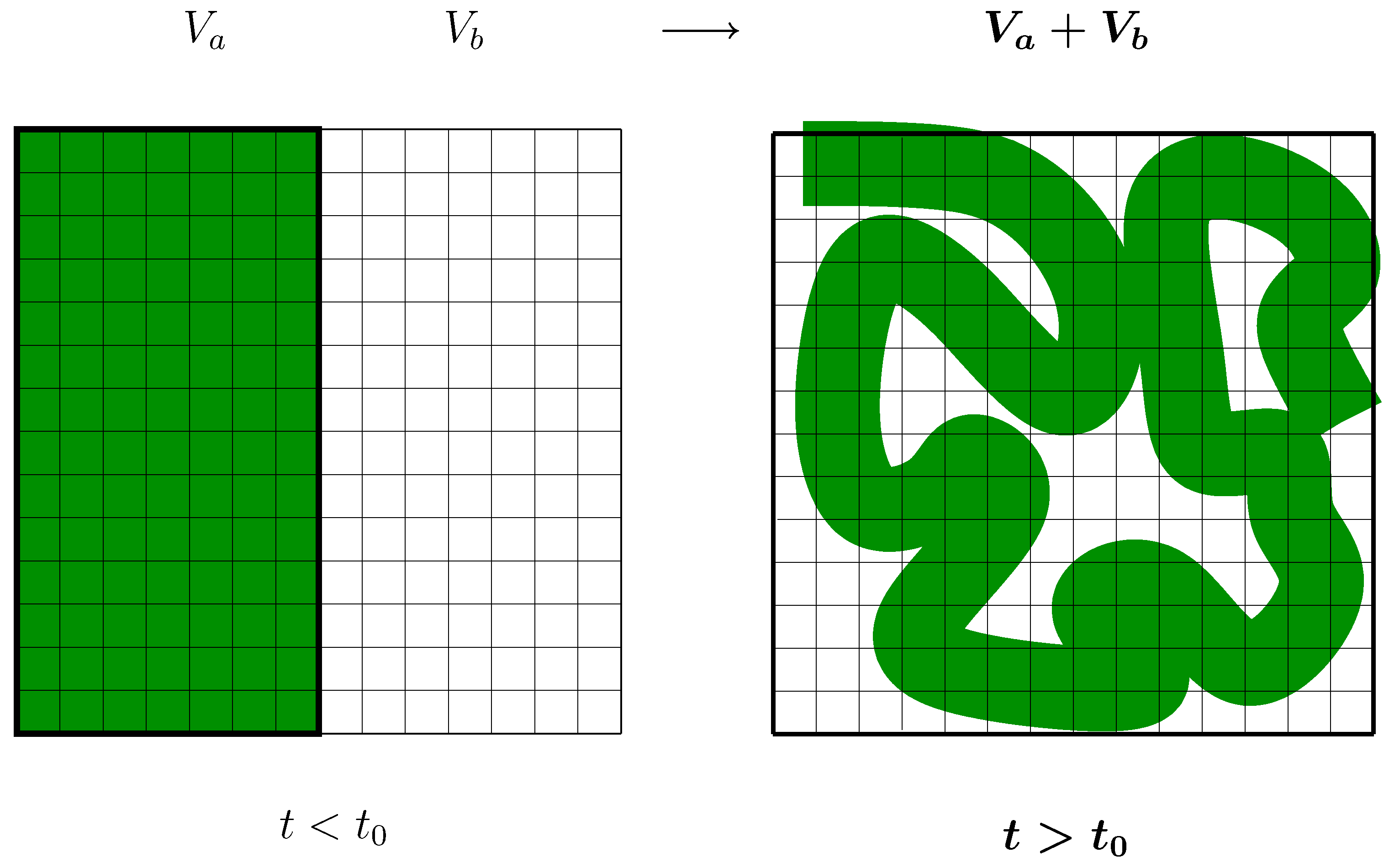
Figure 8. The compact set $\mathit{M}\left({\mathit{t}}_{\mathbf{0}}\right)$, left side, develops into an increasingly folded “spaghetti”-like distribution in phase-space with rising time t, Gibbs’ ”ink-lines”. The right figure shows only the early form of the distribution. At much larger times it will become more and more fractal and finally dense in the new phase space. The grid illustrates the boxes of the box-counting method. All boxes which overlap with $\mathit{M}\left(\mathit{t}\right)$ are counted in N_δ in eq.(20)

Figure 8. The compact set $\mathit{M}\left({\mathit{t}}_{\mathbf{0}}\right)$, left side, develops into an increasingly folded “spaghetti”-like distribution in phase-space with rising time t, Gibbs’ ”ink-lines”. The right figure shows only the early form of the distribution. At much larger times it will become more and more fractal and finally dense in the new phase space. The grid illustrates the boxes of the box-counting method. All boxes which overlap with $\mathit{M}\left(\mathit{t}\right)$ are counted in N_δ in eq.(20)

This is illustrated by the following figure (8). With this extension of eq.(5) Boltzmann’s entropy (6) is at time t ≫ t₀ equal to the logarithm of the larger phase space W (E, N, V₂). This is the second law of thermodynamics. The box-counting is also used in the definition of the Kolmogorov entropy, the average rate of entropy gain [20, 21]. Of course still at $t_0\overline{\mathcal{M}\left(t_0\right)}=\mathcal{M}\left(t_0\right)=\mathcal{E}\left(N,V_1\right)$:

$$\begin{array}{ccc}\hfill M\left(E,N,t_0\right)& =& B{\displaystyle \int d_{\left\{q_0\subset V_1\right\}}\frac{1}{N!}{\left(\frac{d^3{q}_0{d}^3{p}_0}{{\left(2\pi \hslash \right)}^3}\right)}^N{є}_0\delta \left(E-{\widehat{H}}_N\right)}\hfill \\ & \equiv & {\displaystyle {\int }_{\left\{q_0\subset V_2\right\}}\frac{1}{N!}{\left(\frac{d^3{q}_0{d}^3{p}_0}{{\left(2\pi \hslash \right)}^3}\right)}^N{є}_0\delta \left(E-{\widehat{H}}_N\right)}\hfill \end{array}$$

(23)

$$\begin{array}{ccc}& =& W\left(E,N,V_1\right).\end{array}$$

(24)

The box-counting volume is analogous to the standard method to determine the fractal dimension of a set of points [20] by the box-counting dimension:

$${\dim }_{box}\mathcal{M}\left(E,N,t\gg t_0\right):={\underset{¯}{\lim }}_{\delta \to 0}\frac{\ln N_{\delta }\left[\mathcal{M}\left(E,N,t\gg t_0\right)\right]}{-\ln \delta }$$

(25)

Like the box-counting dimension, vol_box has the peculiarity that it is equal to the volume of the smallest closed covering set. E.g.: The box-counting volume of the set of rational numbers {Q} between 0 and 1, is vol_box{Q} = 1, and thus equal to the measure of the real numbers, c.f. Falconer [20] section 3.1. This is the reason why vol_box is not a measure in its strict mathematical sense because then we should have

$${\text{vol}}_{box}\left[{\displaystyle \sum _{i\subset \left\{\mathbf{Q}\right\}}\left({\mathcal{M}}_i\right)}\right]={\displaystyle \sum _{i\subset \left\{\mathbf{Q}\right\}}{\text{vol}}_{box}\left[{\mathcal{M}}_i\right]}=0,$$

(26)

therefore the quotation marks for the box-counting “measure” c.f. appendix 7.

Coming back to the the end of section (5.1), the volume W (A, B, ⋯, t) of the relevant ensemble, the closure $\overline{\mathcal{M}\left(t\right)}$ must be “measured” by something like the box-counting “measure” (20,21) with the box-counting integral $B{\displaystyle \int d}$ which must replace the integral in eq.(5). Due to the fact that the box-counting volume is equal to the volume of the smallest closed covering set, the new, extended, definition of the phase-space integral eq.(21) is for compact sets like the equilibrium distribution $\mathcal{E}$ identical to the old one eq.(5) and nothing changes for equilibrium statistics. Therefore, one can simply replace the old Boltzmann-definition of the number of complexions and with it of the entropy by the new one (21).

5.3 Conclusion of the discussion of the second law

Macroscopic measurements $\widehat{M}$ determine only a very few of all 6N d.o.f. Any macroscopic theory like thermodynamics deals with the volumes M of the corresponding closed sub-manifolds $\overline{\mathcal{M}}$ in the 6N-dim. phase space not with single points. The averaging over ensembles or finite sub-manifolds in phase space becomes especially important for the microcanonical ensemble of a finite system.

Because of this necessarily coarsed and redundant information, macroscopic measurements, and with it also macroscopic theories are unable to distinguish fractal sets $\mathcal{M}$ from their closures $\overline{\mathcal{M}}$. Therefore, I make the conjecture: the proper manifolds determined by a macroscopic theory like thermodynamics are the closed $\overline{\mathcal{M}}$. However, an initially closed subset of points at time t₀ does not necessarily evolve again into a closed subset at t ≫ t₀. I.e. the closure operation and the t → ∞ limit do not commute, and the macroscopic dynamics becomes thus irreversible.

Here is the origin of the misunderstanding by the famous reversibility paradoxes which were invented by Loschmidt [22] and Zermelo [23, 24] and which bothered Boltzmann so much [25, 26]. These paradoxes address to trajectories of single points in the N-body phase space which must return after Poincarre’s recurrence time or which must run backwards if all momenta are exactly reversed. Therefore, Loschmidt and Zermelo concluded that the entropy should decrease as well as it was increasing before. The specification of a single point demands of course a microscopic exact specificationof all 6N degrees of freedom not a determination of a few macroscopic degrees of freedom only. No entropy is defined for a single point. Moreover, it is highly unlikely that all points in the micro-ensemble have commensurate recurrence times so that they can return simultaneously to their initial positions. Once the manifold has spread over the larger phase space it will never return.

This way various non-trivial limiting processes are avoided. Neither does one invoke the thermodynamic limit of a homogeneous system with infinitely many particles nor does one rely on the ergodic hypothesis of the equivalence of (very long) time averages and ensemble averages. The use of ensemble averages is justified directly by the very nature of macroscopic (incomplete) measurements. Coarse-graining appears as natural consequence of this. The box-counting method mirrors the averaging over the overwhelming number of non-determined degrees of freedom. Of course, a fully consistent theory must use this averaging explicitly. Then one would not depend on the order of the limits lim_δ→0 lim_t→∞ as it was tacitly assumed here. Presumably, the rise of the entropy can then be already seen at finite times when the fractality of the distribution in phase space is not yet fully developed. The coarse-graining is no more a mathematical ad hoc assumption. Moreover the second law is in the EPS-formulation of statistical mechanics not linked to the thermodynamic limit as was thought up to now [14, 15, 1].

6 Final conclusion

Entropy has a simple and elementary definition by the area e^{S(E, N, ⋯)} of the microcanonical ensem-ble in the 6N dim. phase space. Canonical ensembles are not equivalent to the micro-ensemble in the most interesting situations:

• at phase-separation (→heat engines !), one gets inhomgeneities, and a negative heat ca-pacity or some other negative susceptibility,
• Heat can flow from cold to hot.
• phase transitions can be localized sharply and unambiguously in small classical or quantum systems, there is no need for finite size scaling to identify the transition.
• also really large self-gravitating systems can now be addressed.

Entropy rises during the approach to equilibrium, ∆S ≥ 0, also for small mixing systems. i.e. the second law is valid even for small systems [2, 3].

With this geometric foundation thermo-statistics applies not only to extensive systems but also to non-extensive ones which have no thermodynamic limit.

7 Appendix

In the mathematical theory of fractals[20] one usually uses the Hausdorff measure or the Hausdorff dimension of the fractal [21]. This, however, would be wrong in Statistical Mechanics. Here I want to point out the difference between the box-counting “measure” and the proper Hausdorff measure of a manifold of points in phase space. Without going into too much mathematical details we can make this clear again with the same example as above: The Hausdorff measure of the rational numbers ∈ [0, 1] is 0, whereas the Hausdorff measure of the real numbers ∈ [0, 1] is 1. Therefore, the Hausdorff measure of a set is a proper measure. The Hausdorff measure of the fractal distribution in phase space $\mathcal{M}\left(t\to \infty \right)$ is the same as that of $\mathcal{M}\left(t_0\right)$, W (E, N, V₁). Measured by the Hausdorff measure the phase space volume of the fractal distribution $\mathcal{M}\left(t\to \infty \right)$ is conserved and Liouville’s theorem applies. This would demand that thermodynamics could distinguish between any point inside the fractal from any point outside of it independently how close it is. This, however, is impossible for any macroscopic theory that can only address the redundant macroscopic information where all unobserved degrees of freedom are averaged over. That is the deep reason why the box-counting “measure” must be taken and where irreversibility comes from.

References

- Goldstein, S.; Lebowitz, J.L. On the (Boltzmann) entropy of nonequilibrium systems. 2003; arXiv:cond-mat/0304251. [Google Scholar]
- Gross, D.H.E. Ensemble probabilistic equilibrium and non-equilibrium thermodynamics without the thermodynamic limit. In Foundations of Probability and Physics; number XIII in PQ-QP: Quantum Probability, White Noise Analysis; Khrennikov, Andrei, Ed.; ACM, World Scientific: Boston, October 2001; pp. 131–146. [Google Scholar]
- Gross, D.H.E. Second law in classical non-extensive systems. In Proceedingsof the First International Conference on Quantum Limits to the Second Law, University of San Diego, 2002; Sheehan, D., Ed.; p. cond{mat/0209467.
- Schrödinger, E. Statistical Thermodynamics, a Course of Seminar Lectures, delivered in January-March 1944 at the School of Theoretical Physics; Cambridge University Press: London, 1946. [Google Scholar]
- Gross, D.H.E.; Votyakov, E. Phase transitions in finite systems = topological peculiarities of the microcanonical entropy surface. 1999, p. 4. http://xxx.lanl.gov/abs/cond-mat/9904073.
- Gross, D.H.E.; Votyakov, E. Phase transitions in ”Small” systems. Eur.Phys.J.B 2000, 15, 115–126. http://arXiv.org/abs/cond-mat/?9911257. [Google Scholar]
- Gross, D.H.E. MicrMicrocanonical thermodynamics: Phase transitions in “Small” systems, volume 66 of Lecture Notes in Physics, World Scientific: Singapore, 2001.
- Bréchignac, C.; Cahuzac, Ph.; Carlier, F.; Leygnier, J.; Roux, J.Ph. J.Chem.Phys. 1995, 102, 1.
- D’Agostino, M.; Gulminelli, F.; Chomaz, Ph.; Bruno, M.; Cannata, F.; Bougault, R.; Gramegna, F.; Iori, I.; le Neindre, N.; Margagliotti, G.V.; Moroni, A.; Vannini, G. Negative heat capacity in the critical region of nuclear fragmentation: an experimental evidence of the liquid-gas phase transition. Phys.Lett.B 2000, 473, 219–225. [Google Scholar]
- Einstein, A. Kinetische Theorie des Wärmegleichgewichtes und des zweiten Hauptsatzes der Thermodynamik. Annalen der Physik 1902, 9, 417–433. [Google Scholar]
- Einstein, A. Eine Theorie der Grundlagen der Thermodynamik. Annalender Physik 1903, 11, 170–187. [Google Scholar]
- Lieb, Elliott H.; Yngvason, J. The physics and mathematics of the second law of thermodynamics. Physics Report,cond-mat/9708200 1999, 310, 1–96. [Google Scholar]
- Lieb, E.H.; Yngvason, J. A guide to entropy and the second law of thermodynamics. mat-ph/9805005, 1998. [Google Scholar]
- Lebowitz, J.L. Microscopic origins of irreversible macroscopic behavior. Physica A 1999, 263, 1–527. [Google Scholar]
- Lebowitz, J.L. Statistical mechanics: A selective review of two central issues. Rev.Mod.Phys. 1999, 71, S346–S357. [Google Scholar]
- Krylov, N.S. Works on the Foundation of Statistical Physics; Princeton University Press: Princeton, 1979. [Google Scholar]
- Fox, R.F. Entropy evolution for the baker map. Chaos 1998, 8, 462–465. [Google Scholar]
- Gilbert, T.; Dorfman, J.R.; Gaspard, P. Entropy production. Phys.Rev.Lett. 2000, 85, 1606, nlin.CD/0003012. [Google Scholar]
- Goldstein, H. Classical Mechanics; Addison-Wesley, Reading, Mass, 1959. [Google Scholar]
- Falconer, Kenneth. Fractal Geometry - Mathematical Foundations and Applications; John Wiley & Sons: Chichester, New York, Brisbane, Toronto,Singapore, 1990. [Google Scholar]
- Weisstein, E.W. Concise Encyclopedia of Mathemetics; CRC Press: London, New York, Washington D.C, 1999. [Google Scholar]
- Loschmidt, J. Wienerberichte 1876, 73, 128.
- Zermelo, E. Wied. Ann. 1896, 57, 778–784.
- Zermelo, E. Über die mechanische Erklärung irreversibler Vorgänge. Wied.Ann. 1897, 60, 392–398. [Google Scholar]
- Cohen, E.G.D. Boltzmann and statistical mechanics. In Boltzmann’s Legacy, 150 Years after his Birth. pages http://xxx.lanl.gov/abs/cond–mat/9608054Rome, 1997; Atti dell Accademia dei Lincei. [Google Scholar]
- Cohen, E.G.D. Boltzmann and Statistical Mechanics, volume 371 of Dynamics: Models and Kinetic Methods for Nonequilibrium Many Body SystemsKluwer: Dordrecht, The Netherlands, e, j. karkheck edition; 2000. [Google Scholar]
- 1How does one normally prove this?: The general link between the microcanonical probability eS(E,N) and the grand-canonical partition function Z(T, µ) for extensive systems is by the Laplace transform:If s(e, n) is concave then there is a single point es, ns withIn the thermodynamic limit (V → ∞) the quadratic approximation in equ.(3) becomes exact and there is a one to one mapping of the microscopic mechanical e = E/V, n = N/V to the intensive T, µ.
- 2In this paper we denote ensembles or manifold in phase space by calligraphic letters like
©2004 by MDPI (http://www.mdpi.org). Reproduction for noncommercial purposes permitted.
Share and Cite
MDPI and ACS Style
Gross, D.H.E. A New Thermodynamics from Nuclei to Stars. Entropy 2004, 6, 158-179. https://doi.org/10.3390/e6010158
AMA Style
Gross DHE. A New Thermodynamics from Nuclei to Stars. Entropy. 2004; 6(1):158-179. https://doi.org/10.3390/e6010158
Chicago/Turabian StyleGross, Dieter H.E. 2004. "A New Thermodynamics from Nuclei to Stars" Entropy 6, no. 1: 158-179. https://doi.org/10.3390/e6010158