A New Approach on Estimation of Solubility and n-Octanol/ Water Partition Coefficient for Organohalogen Compounds

1
School of Chemistry and Chemical Engineering, Central South University, Changsha, 410083, P. R. of China
2
School of Chemistry and Chemical Engineering, Hunan University of Science and Technology, Xiangtan, 411201, P. R. of China
*
Author to whom correspondence should be addressed.
Int. J. Mol. Sci. 2008, 9(6), 962-977; https://doi.org/10.3390/ijms9060962
Submission received: 7 April 2008
/
Revised: 19 May 2008
/
Accepted: 19 May 2008
/
Published: 2 June 2008
(This article belongs to the Section Physical Chemistry, Theoretical and Computational Chemistry)
Abstract
:The aqueous solubility (logW) and n-octanol/water partition coefficient (logPOW) are important properties for pharmacology, toxicology and medicinal chemistry. Based on an understanding of the dissolution process, the frontier orbital interaction model was suggested in the present paper to describe the solvent-solute interactions of organohalogen compounds and a general three-parameter model was proposed to predict the aqueous solubility and n-octanol/water partition coefficient for the organohalogen compounds containing nonhydrogen-binding interactions. The model has satisfactory prediction accuracy. Furthermore, every item in the model has a very explicit meaning, which should be helpful to understand the structure-solubility relationship and may be provide a new view on estimation of solubility.
1. Introduction
Aqueous solubility (logW) and n-octanol/water partition coefficient (logPOW) of compounds have long been recognized as the key molecular properties and are widely used in such diverse areas as pharmaceutics, biochemistry, environmental chemistry, toxicology, chemistry and chemical engineering. Drug delivery, transport, and distribution; prediction of environmental fate; and development of analytical methods depend on solubility and partition properties [1, 2]. As a consequence, it is of considerable value to have practical knowledge of the logW and logPOW values for molecules. The measurement of logW or logPOW through the synthesis of a compound and then its subsequent experimental determination is time-consuming and expensive. Hence, there is strong interest in the structure-based prediction of logW or logPOW for rational development of new drugs and for reasonable assessment of the environmental impact of chemicals before they were released into the environment. Not surprisingly, numerous methods for the prediction of aqueous solubility or partition coefficients have been suggested in the literature [3–19]. Fortunately, Jorgensen did a very good review on the prediction methods of logW for organic compounds [20]. Recently, Kühne has made a comparison among those widely used methods and pointed out that “every method has its method-specific application domains” [21]. Thus, new methods for supplementing existing approaches are required.
It is well known that organohalogen compounds have been manufactured and used in the chemical industry as solvents, propellants, additives, cooling agents, and insecticides for many years [22]. In addition, these compounds can be formed during combustion processes in waste incineration. Generally, organohalogen compounds, such as polychlorinated biphenyls (PCBs), polybrominated biphenyls (PBBs), polychlorinated benzenes, polybrominated benzenes and polychlorinated naphthalenes (PCNs) and so on, have some extent negative impact on the environment and the ecology. Thus the assessment of the environmental risk of these compounds, which can be roughly done by studying their logW or logPOW, is very important. Recently, Padmanabhan [23], Lü [24], and Zou [25] proposed QSPR models to predict the logPOW of PCBs, and obtained good prediction accuracy. In the present paper, based on an understanding of the processes involved in dissolution, a new and very simple method was suggested to predict the logPOW and logW for some halogen containing organic compounds. The present method has a good prediction accuracy and every term in the presented equation has an explicit physical and chemical meaning.
2. Methodology
The dissolution of a solute in a solvent can conceptually take place in two stages: (i) a sizable hole or cavity has to be formed in the solvent phase to accommodate the solute molecule; (ii) the solute molecule is then inserted into the hole, and then interacts with the solvent molecules around it. After the above two steps, a stable solution is formed [26].
At the first stage of the dissolution, an input energy or enthalpy (Einput) is needed to separate the solvent molecules, i.e., to overcome the solvent-solvent cohesive interactions. This energy is proportional to the size or volume of the solute molecule. The second stage of the dissolution is an exothermic process. The output energy (Eoutput) in this stage for organic compounds having no (or very weak) hydrogen-binding interactions with solvent molecules, is, in our opinion, correlated with the interaction of the frontier orbitals of the solute molecules (FMOsolute) and solvent molecules (FMOsolvent). In other words, ignoring the interaction of the hydrogen-binding interactions resulting from solute and solvent molecules, Eoutput is mainly determined by the interactions between solvent’s HOMO (HOMOsolvent) and solute’s LUMO (LUMOsolute), and between solute’s HOMO (HOMOsolute) and solvent’s LUMO (LUMOsolvent), viz.:
According to the above statements, the following equation was proposed to predicted the logW for the organohalogen compounds having no (or very weak) hydrogen-binding interactions with solvent,
where, EHOMOsolute, ELUMOsolute, EHOMOsolvent, and ELUMOsolvent are the energies of the HOMOs and LUMOs of solute and solvent molecule, respectively. For a solvent of interest, e.g. water, its frontier orbitals energies are given. The last term in Eq. (2a) is an invariable, thus Eq. (2a) can be rewritten as:
Here, a, b, c and d are the coefficients; V, EHOMO and ELUMO are the volume, the HOMO energy and the LUMO energy of the solute, respectively. The parameter V of a solute can be calculated by additive method, for the details one should consult Ref. [10]; The EHOMO and ELUMO were calculated by Gaussian 98 program (using Gaussian program packages in SYBYL 6.7 of Tripos, Inc.) at the HF/6-31G(d) level.
3. Regression Analysis
3.1. Aqueous Solubility of PCBs
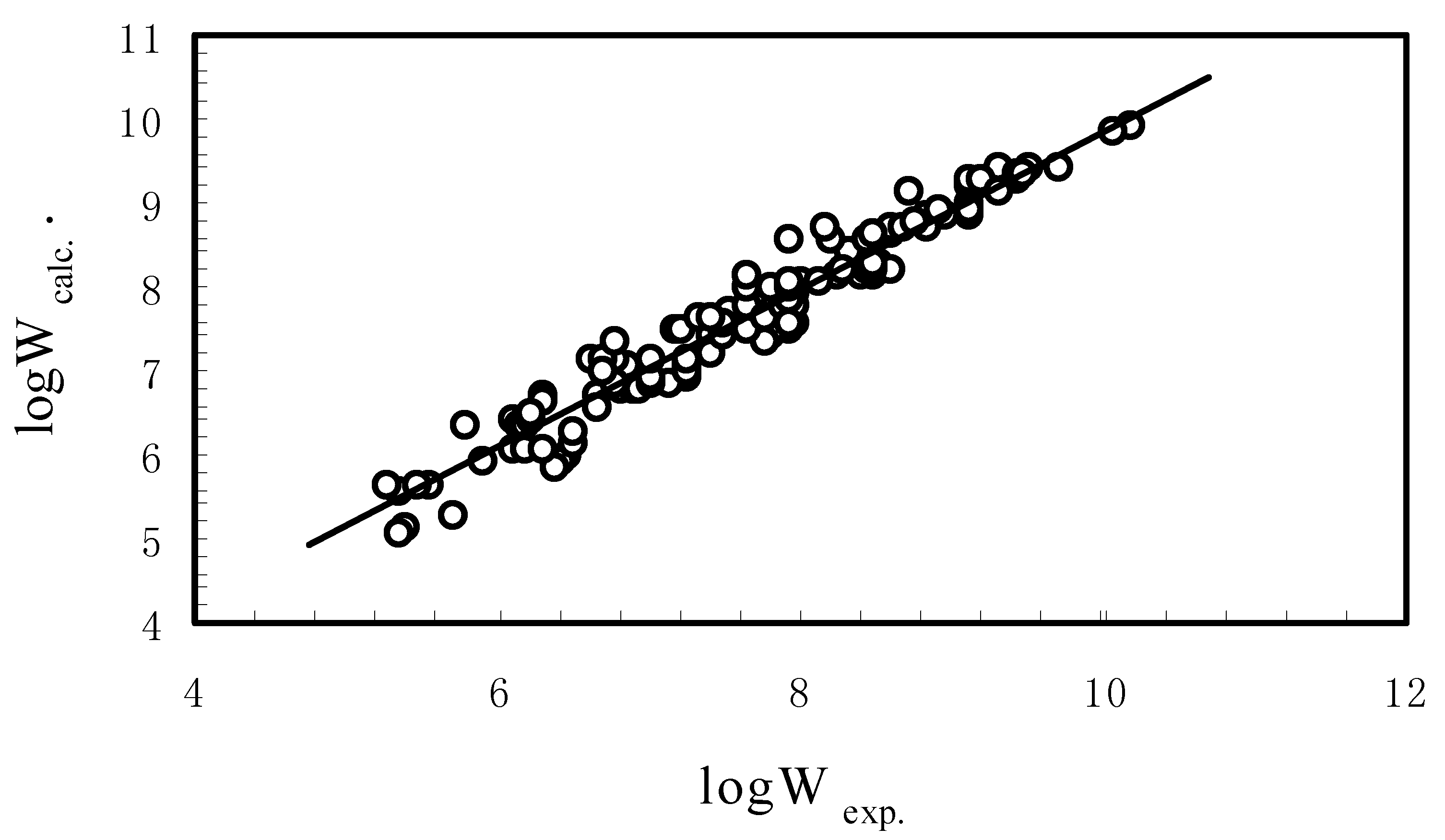
Taking some experimental logW of PCBs [11] (listed in Table 1) as the training set, we employed Eq. (2b) to carry out a regression analysis and got the following equation:
where, R is the correlation coefficient, S is the standard error between the experimental and estimated logW by Eq. (3), n is the number of the sample in the training set. Figure 1 is the plot of the experimental versus the calculated aqueous solubility of PCBs by Eq. (3). From the R and S value of Eq. (3) and Fig. 1, one can see that Eq. (3) has a good correlation.
The characteristics and interrelations of descriptors in Eq. (3) are given in Tables 2 and 3, respectively, which suggested that the three descriptors (V, EHOMO, and ELUMO) are significant descriptors and not strongly correlated with each other. According to the t-test values (in Table 2), the more significant descriptor appearing in Eq. (3) is the descriptor V, which indicated that the volume of PCB molecules is the predominant factor determining the PCB’s aqueous solubility. The t-score value of parameter ELUMO implied that the interaction of LUMO of PCB molecule with the HOMO of water is also play a very importance role in the determination of the PCB’s aqueous solubility.
3.2. n-Octanol/Water Partition Coefficient of PCBs
Hantsch et al. [27] have indicated that there exists a linear relationship between the aqueous solubility (logW) and the n-octanol/water partition coefficient (logPOW) of a solute. As Eq. (2b) can express well the relationship of the structure-aqueous solubility for PCB congeners, it was also expected to be able to predict the n-octanol/water partition coefficient. Thus, taking some experimental logPOW of PCBs [10, 23] (see Table 1) as the training set, we employed Eq. (2b) to carry out the regression analysis and got the following equation:
Equation (4) has a high correlation coefficient R and small standard deviation S for predicting the n-octanol/water partition coefficient of PCB congeners.
4. Discussion
A closer analysis of the coefficients in front of the parameters in Eq. (3) can provide physical insights to understand structure-solubility relationship. The negative coefficient of the parameter V implied that the PCB molecule with a larger volume has a smaller logW value than that of the smaller PCB. That is to say, the larger PCB has lower solubility in water than that of the smaller PCB, because a larger hole has to be carved in the water layer for accepting the larger PCB molecule, which needs a larger energy input. The positive coefficient of EHOMO means that the higher the HOMO of the PCB molecule, the larger the logW value of the PCB is. In our opinion, the higher energy of HOMO of the solute can interact with the LUMO of water more effectively, which is more energetically favorable for the formation of the solution. Thus the higher the HOMO of the PCB molecule, the more soluble it is. The higher the energy of LUMO of the solute molecule, the more effectively the LUMO of the solute molecule interact with the HOMO of water. Thus, the solubility of PCBs increases with the increase of the ELUMO values.
In order to test the robustness and prediction ability of Eq. (3), a cross-validation analysis was performed. In the cross-validation analysis, a model is calculated with groups of objects (i.e., PCB congeners) omitted subsequently, followed by the prediction of the logW for the omitted objects. In the present study, Leave-One-Out (LOO) cross-validation method is employed. The internal predicted ability and the robustness of the models are characterized in terms of the corresponding leave-one-out cross-validation correlation coefficient (RCV) and the cross-validation predicted standard error (SCV), which are defined as:
where yi and ŷi are the experimental and predicted value, respectively. ȳ is the mean value of yi.
Recently, Padmanabhan et al. [23], and Lü et al. [24] developed the QSPR models for estimating logPOW of 133 PCB congeners with prediction errors of 0.225 and 0.205 log units, respectively. In order to compare with Padmanabhan’s and Lü’s work, we employed the same data set used in their work and employed Eq.(2b) to perform the correlation analysis, namely:
The results of Eq. (4) and Eq. (7) showed that the predicted accuracy of the present model is better than that of Padmanabhan’s QSPR model and is comparable to that of Lü’s model. Examination of Eq. (4) or Eq. (7) may lead to the following significant interpretations: the value of logPOW increases with the increase of V, which means that increase in solute size, V, favors wet octanol phase. The reason is that water molecule is more polar than the n-octanol molecule, so the cohesive energy is larger between water molecules than that between the n-octanol ones. Thus, more energy input is needed to create a similarly-sized hole in the more polar solvent (i.e., water phase) than that in the less polar solvent (i.e., n-octanol phase). Consequently, the PCB molecule tends to enter into the n-ocatanol phase, which is energetically more favorable. Increase the EHOMO or ELUMO solute favors the aqueous layer.
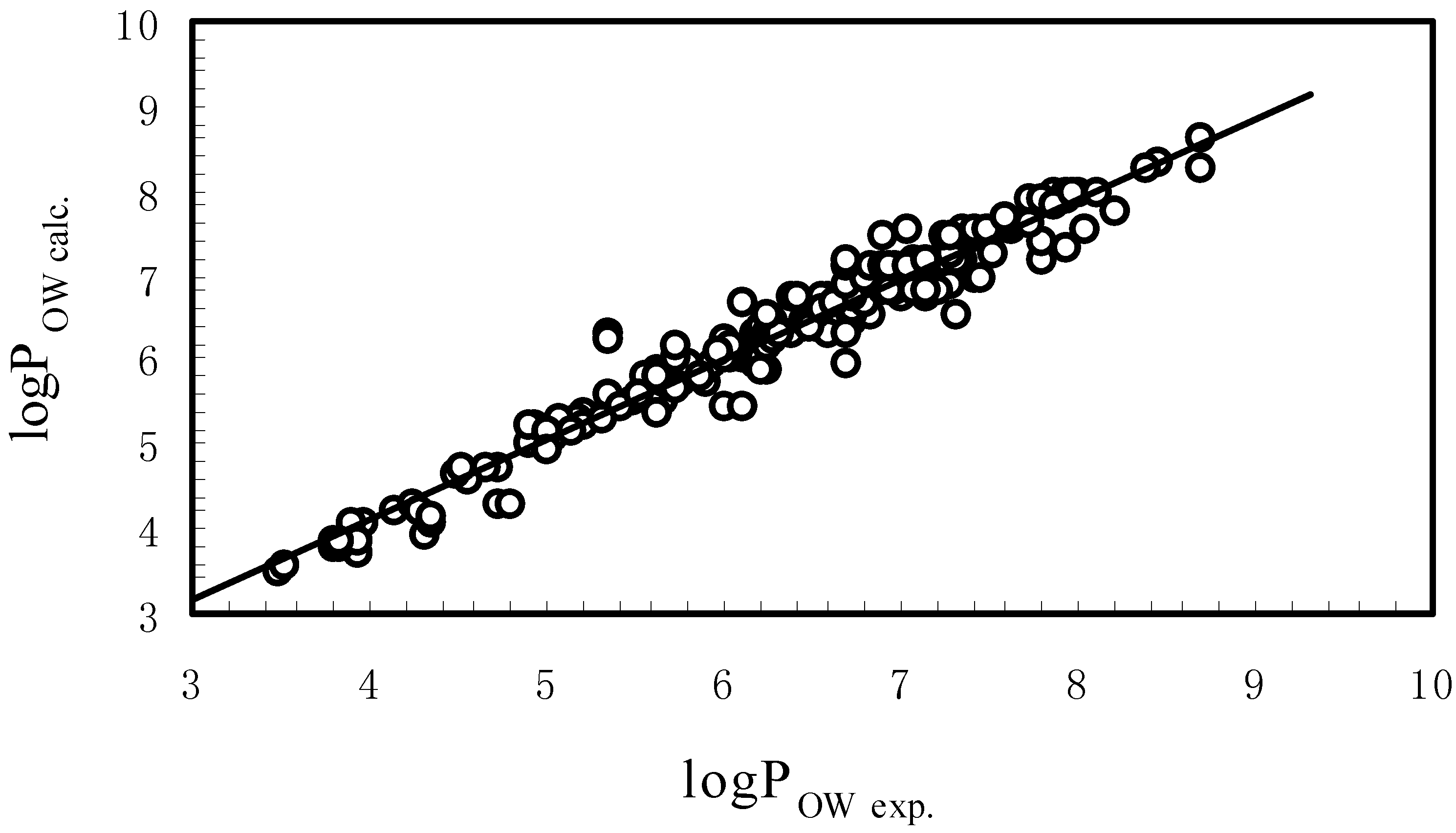
It is relatively easy to build a QSPR model for the congeners, while it is somewhat difficult to correlate a data set of heterogeneous compounds. Besides having a high correlation and low deviation, a valuable QSPR model should also have a large application range. Thus, in order to verify the application of Eq. (2) in more complex data sets, we combined the logPOW of 157 PCBs and some other halogen substituted aromatic compounds [10, 11] (including PBBs, PCNs, and HBs, listed in Table 1) as a data set, and used Eq. (2b) to perform a correlation analysis, the following correlation equation was obtained:
Figure 2 is the plot of experimental logPOW versus the calculated ones by Eq. (8), which shows that Eq. (8) has a good correlation and prediction ability. The standard deviation of the correlation equation is only 0.247 log units, which is within the experimental uncertainties. The result of Eq. (8) showed that the model (i.e., Eq. (2b)) can be employed to predict logW or logPOW for a wide range compounds with various structures.
It should be noted that some excellent software (such as ACD/LogP, CLogP [28], and so on) have been developed to compute logPOW. In order to compare the presented results with the data calculated by these softwares, some leading compounds were selected (see Table 4) and their logPOW were computed by Eq. (8) and by CLogP software (using CLogP packages in SYBYL 6.7 of Tripos, Inc.), respectively. For these compounds in Table 4, the average absolute deviation is 0.45 log units between the experimental logPOW exp. and the logPOW CLogP calculated by CLogP software. While, for the same compounds in Table 4, the average absolute deviation is only 0.14 log units between the logPOW exp. and the logPOW calc. predicted by Eq. (8). Seen from the average absolute deviation, the precision of present method is a little better than that of CLogP software.
5. Conclusions
Based on the comprehension of the dissolution process, a very simple three-parameter model was proposed to predict the aqueous solubility and n-octanol/water partition coefficients for organohalogen compounds containing nonhydrogen-binding interactions. The model has satisfactory prediction accuracy. Furthermore, every item in the model has a very explicit meaning, which would be helpful to understand the structure-solubility relationships.
Acknowledgment
The Project was supported by the National Natural Science Foundation of China (Grant No. 20772028) and the Natural Science Foundation of Hunan (Grant No. 06JJ2002).
References and Notes
- Hantsch, C. Quantitative approach to biochemical structure-activity relationships. Acc. Chem. Res. 1969, 2, 232–239. [Google Scholar]
- Bodor, N; Huang, MJ. A new method for the estimation of the aqueous solubility of organic compounds. J. Pharm. Sci. 1992, 81, 954–960. [Google Scholar]
- Hansch, C; Leo, A. Substituent Constant for Correlation in Chemical and Biology; Wiley-Interscience: New York, NY, USA, 1979. [Google Scholar]
- Cao, C; Li, ZL. Molecular Polarizability. 1. Relationship to Water Solubility of Alkanes and Alcohols. J. Chem. Inf. Comput. Sci. 1998, 38, 1–7. [Google Scholar]
- Bodor, N; Gabanyi, Z; Wong, CK. A new method for the estimation of partition coefficient. J. Am. Chem. Soc. 1989, 111, 3783–3786. [Google Scholar]
- Jain, N; Yalkowsky, SH. UPPER III: Unified physical property estimation relationships. Application to non-hydrogen bonding aromatic compounds. J. Pharm. Sci. 1999, 88, 852–860. [Google Scholar]
- Huuskonen, JJ; Villa, AEP; Tetko, IV. Prediction of partition coefficient based on atom-type electrotopological state indices. J. Pharm. Sci. 1999, 88, 229–233. [Google Scholar]
- Hall, LH; Kier, LB. Electrotopological State Indices for Atom Types: A Novel Combination of Electronic, Topological, and Valence State Information. J. Chem. Inf. Comput. Sci. 1995, 35, 1039–1045. [Google Scholar]
- Abraham, MH. Scales of solute hydrogen-bonding: their construction and application to physicochemical and biochemical processes. Chem. Soc. Rev. 1993, 22, 73–83. [Google Scholar]
- Ruelle, P. The n-octanol and n-hexane/water partition coefficient of environmentally relevant chemicals predicted from the mobile order and disorder (MOD) thermodynamics. Chemosphere 2000, 40, 457–512. [Google Scholar]
- Wang, X; Tang, S; Liu, S; et al. Molecular Hologram Derived Quantitative Structure–Property Relationships to Predict Physico-Chemical Properties of Polychlorinated Biphenyls. Chemosphere 2003, 51, 617–632. [Google Scholar]
- Staikova, M; Wania, F; Donaldson, DJ. Molecular polarizability as a single-parameter predictor of vapour pressures and octanol–air partitioning coefficients of non-polar compounds: a priori approach and results. Atmos. Environ. 2004, 38, 213–225. [Google Scholar]
- Gramatica, P; Navas, N; Todeschini, R. 3D-modelling and prediction by WHIM descriptors. Part 9. Chromatographic relative retention time and physico-chemical properties of polychlorinated biphenyls (PCBs). Chemometr. Intell. Lab. 1998, 40, 53–63. [Google Scholar]
- Hansen, BG; Paya-Perez, AB; Rahman, M; Larsen, BR. QSARs for KOW and KOC of PCB congeners: a critical examination of data, assumptions and statistical approaches. Chemosphere 1999, 39, 2209–2228. [Google Scholar]
- Tolls, J; van Dijk, J; Verbruggen, EJM; et al. Aqueous Solubility-Molecular Size Relationships: A Mechanistic Case Study Using C10- to C19-Alkanes. J. Phys. Chem. A. 2002, 106, 2760–2765. [Google Scholar]
- Kamlet, MJ; Doherty, RM; Abraham, MH; et al. Linear solvation energy relationship. 46. An improved equation for correlation and prediction of octanol/water partition coefficients of organic nonelectrolytes (including strong hydrogen bond donor solutes). J. Phys. Chem. 1988, 92, 5244–5255. [Google Scholar]
- Huang, J; Yu, G; Zhang, ZL; et al. Application of TLSER method in predicting the aqueous solubility and n - octanol/water partition coefficient of PCBs, PCDDs and PCDFs. J. Environ. Sci. 2004, 16, 21–29. [Google Scholar]
- Lin, ZH; Liu, SS; Li, ZL; et al. QSPR Study on Solubility and Octanol/Water Partition Coefficients of Hydrocarbons by Molecular Distance-Edge Vector. Environ. Chem. 2000, 19, 528–537. (in Chinese). [Google Scholar]
- Dai, JY; Chen, L; Zhao, JF. Prediction of partition property of polychlorinated organic compounds using linear solvation energy parameter. China Environ. Sci. 2002, 22, 329–333. (in Chinese). [Google Scholar]
- Jorgensen, WL; Duffy, EM. Prediction of drug solubility from structure. Adv. Drug Deliver. Rev. 2002, 54, 355–366. [Google Scholar]
- Kühen, R; Ebert, RU; Schüürmann, G. Model Selection Based on Structural Similarity-Method Description and Application to Water Solubility Prediction. J. Chem. Inf. Model. 2006, 46, 636–641. [Google Scholar]
- Ballschmiter, KH; Haltrich, W; Kühn, W; et al. HOV-Studie: Halogenorganische Verbindungen in Gewässern; Fachgruppe Wasserchemie der Gesellschaft Deutscher Chemiker: Frankfurt, 1987. [Google Scholar]
- Padmanabhan, J; Parthasarathi, R; Subramanian, V; Chattaraj, PK. QSPR models for polychlorinated biphenyls: n-Octanol/water partition coefficient. Bioorg. Med. Chem. 2006, 14, 1021–1028. [Google Scholar]
- Lü, WJ; Chen, YL; Liu, MC; et al. QSPR prediction of n-octanol/water partition coefficient for polychlorinated biphenyls. Chemosphere 2007, 69, 469–478. [Google Scholar]
- Zuo, JW; Jiang, YJ; Hu, GX; et al. QSPR/QSAR Studies on the Physicochemical Properties and Biological Activities of Polychlorinated Biphenyls. Acta Phys.-Chim. Sin. 2005, 21, 267–272. (in Chinese). [Google Scholar]
- Kamlet, MJ; Doherty, RM; Abboud, JLM; et al. Solubility–a new look. Chemtech 1986, 16, 566–576. [Google Scholar]
- Hansch, C; Quinlan, JE; Lawrence, GL. Linear free-energy relationship between partition coefficients and the aqueous solubility of organic liquids. J. Org. Chem. 1968, 33, 347–350. [Google Scholar]
- Chou, JT; Jurs, PC. Computer-Assisted Computation of Partition Coefficients from Molecular Structures Using Fragment Constants. J. Chem. Inf. Comput. Sci. 1979, 19, 172–178. [Google Scholar]
Figure 1.
The plot of experimental aqueous solubility vs. the ones calculated by Eq. (3)
Figure 1.
The plot of experimental aqueous solubility vs. the ones calculated by Eq. (3)

Figure 2.
The plot of experimental n-octanol/water partition coefficient vs. the ones calculated by Eq. (8).
Figure 2.
The plot of experimental n-octanol/water partition coefficient vs. the ones calculated by Eq. (8).


Table 1.
The aqueous solubility (logW) and n-octanol/water partition coefficient (logPOW) of some organohalogen compounds.
| Substitution patterns | V | EHOMO (a.u.) | ELUMO (a.u.) | -logWexp.a | logPOW exp.b | -logWcalc.c | logPOW calc.d | -ΔlogWe | ΔlogPOWe |
|---|---|---|---|---|---|---|---|---|---|
| Chlorobiphenyls | |||||||||
| 2- | 172.9 | −0.31684 | 0.11773 | 4.38 | 4.82 | 4.55 | −0.17 | ||
| 3- | 172.9 | −0.31044 | 0.10490 | 5.39 | 4.66 | 5.15 | 4.71 | 0.24 | −0.05 |
| 4- | 172.9 | −0.30610 | 0.10507 | 5.33 | 4.63 | 5.08 | 4.67 | 0.25 | −0.04 |
| 2,2’- | 185.8 | −0.33398 | 0.12177 | 5.72 | 4.72 | 5.31 | 4.89 | 0.41 | −0.17 |
| 2,3- | 185.8 | −0.32596 | 0.10991 | 5.35 | 4.99 | 5.58 | 5.02 | −0.23 | −0.03 |
| 2,3’- | 185.8 | −0.32760 | 0.10802 | 5.26 | 4.84 | 5.66 | 5.07 | −0.40 | −0.23 |
| 2,4- | 185.8 | −0.32248 | 0.10594 | 5.56 | 5.15 | 5.66 | 5.06 | −0.10 | 0.09 |
| 2,4’- | 185.8 | −0.32189 | 0.10697 | 5.46 | 5.09 | 5.62 | 5.04 | −0.16 | 0.05 |
| 2,5- | 185.8 | −0.32464 | 0.10552 | 5.00 | 5.70 | 5.09 | −0.09 | ||
| 2,6- | 185.8 | −0.33322 | 0.11642 | 4.93 | 5.47 | 4.97 | −0.04 | ||
| 3,3’- | 185.8 | −0.32076 | 0.09420 | 6.45 | 5.27 | 6.02 | 5.25 | 0.43 | 0.02 |
| 3,4- | 185.8 | −0.31429 | 0.09528 | 6.39 | 5.23 | 5.89 | 5.17 | 0.50 | 0.06 |
| 3,4’- | 185.8 | −0.31601 | 0.09419 | 6.40 | 5.15 | 5.95 | 5.21 | 0.45 | −0.06 |
| 3,5- | 185.8 | −0.32035 | 0.09364 | 5.40 | 6.03 | 5.25 | 0.15 | ||
| 4,4’- | 185.8 | −0.31190 | 0.09439 | 6.37 | 5.23 | 5.88 | 5.17 | 0.49 | 0.06 |
| 2,2’,3- | 198.7 | −0.33898 | 0.11209 | 6.10 | 5.12 | 6.07 | 5.36 | 0.03 | −0.24 |
| 2,2’,4- | 198.7 | −0.34012 | 0.11041 | 6.49 | 5.39 | 6.14 | 5.40 | 0.35 | −0.01 |
| 2,2’,5- | 198.7 | −0.33646 | 0.11028 | 6.17 | 5.33 | 6.09 | 5.37 | 0.08 | −0.04 |
| 2,2’,6- | 198.7 | −0.33558 | 0.11438 | 5.90 | 5.04 | 5.94 | 5.29 | −0.04 | −0.25 |
| 2,3,3’- | 198.7 | −0.33701 | 0.10200 | 5.60 | 6.37 | 5.52 | 0.08 | ||
| 2,3,4- | 198.7 | −0.32989 | 0.09988 | 6.18 | 5.68 | 6.33 | 5.49 | −0.15 | 0.19 |
| 2,3,4’- | 198.7 | −0.33020 | 0.10032 | 5.80 | 5.29 | 6.32 | 5.49 | −0.52 | −0.20 |
| 2,3,6- | 198.7 | −0.33795 | 0.10464 | 6.49 | 5.44 | 6.29 | 5.48 | 0.20 | −0.04 |
| 2,3’,4- | 198.7 | −0.33268 | 0.09730 | 6.11 | 5.54 | 6.46 | 5.56 | −0.35 | −0.02 |
| 2,3’,5- | 198.7 | −0.33037 | 0.09875 | 6.14 | 5.65 | 6.38 | 5.52 | −0.24 | 0.13 |
| 2,4,4’- | 198.7 | −0.33669 | 0.09729 | 6.22 | 5.71 | 6.52 | 5.59 | −0.30 | 0.12 |
| 2,4,5- | 198.7 | −0.33641 | 0.10953 | 5.74 | 6.11 | 5.38 | 0.36 | ||
| 2,4,6- | 198.7 | −0.32716 | 0.09635 | 5.50 | 6.41 | 5.53 | −0.03 | ||
| 2,4’,5- | 198.7 | −0.32866 | 0.09554 | 6.18 | 5.68 | 6.46 | 5.56 | −0.28 | 0.12 |
| 2,4’,6- | 198.7 | −0.33949 | 0.10293 | 6.16 | 5.24 | 6.37 | 5.52 | −0.21 | −0.28 |
| 2,3’,4’- | 198.7 | −0.32913 | 0.09591 | 6.21 | 5.71 | 6.45 | 5.55 | −0.24 | 0.16 |
| 2,3’,5’- | 198.7 | −0.33555 | 0.10933 | 6.30 | 5.71 | 6.11 | 5.38 | 0.19 | 0.33 |
| 3,3’,5- | 198.7 | −0.33039 | 0.08369 | 5.70 | 6.87 | 5.77 | −0.07 | ||
| 3,4,4’- | 198.7 | −0.31950 | 0.08533 | 5.22 | 6.66 | 5.65 | −0.43 | ||
| 2,2’,3,3’- | 211.6 | −0.34469 | 0.10442 | 6.83 | 5.67 | 6.77 | 5.80 | 0.06 | −0.13 |
| 2,2’,3,4- | 211.6 | −0.34347 | 0.10180 | 7.00 | 5.79 | 6.84 | 5.84 | 0.16 | −0.05 |
| 2,2’,3,4’- | 211.6 | −0.34602 | 0.10288 | 6.96 | 5.72 | 6.84 | 5.84 | 0.12 | −0.12 |
| 2,2’,3,5’- | 211.6 | −0.34073 | 0.10278 | 6.91 | 5.73 | 6.76 | 5.80 | 0.15 | −0.07 |
| 2,2’,3,6- | 211.6 | −0.33988 | 0.10317 | 6.30 | 4.84 | 6.74 | 5.78 | −0.44 | −0.94 |
| 2,2’,3,6’- | 211.6 | −0.34164 | 0.10791 | 6.30 | 4.84 | 6.61 | 5.72 | −0.31 | −0.88 |
| 2,2’,4,4’- | 211.6 | −0.34756 | 0.10135 | 7.23 | 5.94 | 6.91 | 5.88 | 0.32 | 0.06 |
| 2,2’,4,5- | 211.6 | −0.34328 | 0.10017 | 6.86 | 5.69 | 6.89 | 5.86 | −0.03 | −0.17 |
| 2,2’,4,5’- | 211.6 | −0.34181 | 0.10125 | 7.12 | 5.87 | 6.83 | 5.83 | 0.29 | 0.04 |
| 2,2’,4,6- | 211.6 | −0.34116 | 0.10154 | 6.94 | 5.75 | 6.81 | 5.82 | 0.13 | −0.07 |
| 2,2’,4,6’- | 211.6 | −0.34355 | 0.10650 | 6.65 | 5.51 | 6.68 | 5.76 | −0.03 | −0.25 |
| 2,2’,5,5’- | 211.6 | −0.34136 | 0.10118 | 7.00 | 5.79 | 6.82 | 5.83 | 0.18 | −0.04 |
| 2,2’,5,6’- | 211.6 | −0.33758 | 0.10649 | 6.65 | 5.55 | 6.60 | 5.71 | 0.05 | −0.16 |
| 2,2’,6,6’- | 211.6 | −0.34062 | 0.11159 | 6.20 | 5.24 | 6.47 | 5.65 | −0.27 | −0.41 |
| 2,3,3’,4- | 211.6 | −0.34043 | 0.09287 | 6.77 | 6.10 | 7.08 | 5.97 | −0.31 | 0.13 |
| 2,3,4,4’- | 211.6 | −0.33393 | 0.09127 | 6.86 | 6.24 | 7.04 | 5.94 | −0.18 | 0.30 |
| 2,3,4,5- | 211.6 | −0.33570 | 0.08962 | 6.05 | 7.12 | 5.98 | 0.07 | ||
| 2,3,4’,5- | 211.6 | −0.33694 | 0.08918 | 6.77 | 6.10 | 7.15 | 6.00 | −0.38 | 0.10 |
| 2,3,4’,6- | 211.6 | −0.33980 | 0.09821 | 7.02 | 5.76 | 6.90 | 5.87 | 0.12 | −0.11 |
| 2,3,5,6- | 211.6 | −0.34219 | 0.09374 | 7.25 | 5.96 | 7.08 | 5.97 | 0.17 | −0.01 |
| 2,3’,4,4’- | 211.6 | −0.33518 | 0.08905 | 6.63 | 5.98 | 7.13 | 5.99 | −0.50 | −0.01 |
| 2,3’,4,5- | 211.6 | −0.33790 | 0.08747 | 6.32 | 7.22 | 6.04 | 0.28 | ||
| 2,3’,4,6- | 211.6 | −0.34162 | 0.09677 | 7.26 | 6.03 | 6.97 | 5.91 | 0.29 | 0.12 |
| 2,3’,4’,5- | 211.6 | −0.33665 | 0.08847 | 6.69 | 6.22 | 7.17 | 6.01 | −0.48 | 0.21 |
| 2,3’,4’,6- | 211.6 | −0.33738 | 0.08940 | 7.02 | 5.76 | 7.15 | 6.00 | −0.13 | −0.24 |
| 2,4,4’,5- | 211.6 | −0.34486 | 0.10227 | 6.77 | 6.10 | 6.84 | 5.84 | −0.07 | 0.26 |
| 2,4,4’,6- | 211.6 | −0.33283 | 0.08676 | 7.26 | 6.03 | 7.17 | 6.01 | 0.09 | 0.02 |
| 2,3’,4’,5’- | 211.6 | −0.34118 | 0.09656 | 6.71 | 5.98 | 6.97 | 5.91 | −0.26 | 0.07 |
| 3,3’,4,4’- | 211.6 | −0.32696 | 0.07703 | 6.21 | 7.40 | 6.12 | 0.09 | ||
| 3,3’,5,5’- | 211.6 | −0.34046 | 0.07418 | 6.10 | 7.70 | 6.28 | −0.18 | ||
| 2,2’,3,3’,6- | 224.5 | −0.34538 | 0.09793 | 6.78 | 5.60 | 7.36 | 6.19 | −0.58 | −0.59 |
| 2,2’,3,4,4’- | 224.5 | −0.35109 | 0.09425 | 7.62 | 6.18 | 7.56 | 6.30 | 0.06 | −0.12 |
| 2,2’,3,4,5- | 224.5 | −0.34736 | 0.09147 | 7.87 | 6.38 | 7.60 | 6.31 | 0.27 | 0.07 |
| 2,2’,3,4,5’- | 224.5 | −0.34484 | 0.09419 | 7.66 | 6.23 | 7.47 | 6.25 | 0.19 | −0.02 |
| 2,2’,3,4,6- | 224.5 | −0.34424 | 0.09240 | 7.92 | 6.50 | 7.52 | 6.27 | 0.40 | 0.23 |
| 2,2’,3,4,6’- | 224.5 | −0.34923 | 0.09995 | 6.78 | 5.60 | 7.35 | 6.18 | −0.57 | −0.58 |
| 2,2’,3,4’,5- | 224.5 | −0.34906 | 0.09275 | 7.82 | 6.32 | 7.58 | 6.31 | 0.24 | 0.01 |
| 2,2’,3,4’,6- | 224.5 | −0.34780 | 0.09405 | 7.17 | 5.87 | 7.52 | 6.27 | −0.35 | −0.40 |
| 2,2’,3,5,5’- | 224.5 | −0.34726 | 0.09667 | 7.82 | 6.32 | 7.43 | 6.22 | 0.39 | 0.10 |
| 2,2’,3,5,6- | 224.5 | −0.34678 | 0.09634 | 7.40 | 6.06 | 7.43 | 6.22 | −0.03 | −0.16 |
| 2,2’,3,5’,6- | 224.5 | −0.34390 | 0.09255 | 7.19 | 5.92 | 7.51 | 6.27 | −0.32 | −0.35 |
| 2,2’,3,4’,5’- | 224.5 | −0.34157 | 0.09673 | 7.76 | 6.30 | 7.34 | 6.17 | 0.42 | 0.13 |
| 2,2’,3,4’,6’- | 224.5 | −0.34292 | 0.10112 | 7.40 | 6.04 | 7.22 | 6.11 | 0.18 | −0.07 |
| 2,2’,4,4’,5- | 224.5 | −0.34864 | 0.09267 | 7.95 | 6.41 | 7.58 | 6.30 | 0.37 | 0.11 |
| 2,2’,4,4’,6- | 224.5 | −0.34908 | 0.09510 | 7.66 | 6.23 | 7.50 | 6.27 | 0.16 | −0.04 |
| 2,2’,4,5,5’- | 224.5 | −0.34567 | 0.09264 | 6.65 | 7.54 | 6.28 | 0.37 | ||
| 2,2’,4,5’,6- | 224.5 | −0.34263 | 0.09516 | 7.47 | 6.11 | 7.41 | 6.21 | 0.06 | −0.10 |
| 2,3,3’,4,4’- | 224.5 | −0.34251 | 0.08561 | 7.52 | 6.79 | 7.72 | 6.37 | −0.20 | 0.42 |
| 2,3,3’,4,5- | 224.5 | −0.34496 | 0.08289 | 7.68 | 6.92 | 7.84 | 6.44 | −0.16 | 0.48 |
| 2,3,3’,4’,6- | 224.5 | −0.34592 | 0.08472 | 7.65 | 6.20 | 7.80 | 6.42 | −0.15 | −0.22 |
| 2,3,3’,5,6- | 224.5 | −0.35128 | 0.08237 | 7.95 | 6.41 | 7.95 | 6.50 | 0.00 | −0.09 |
| 2,3,3’,5’,6- | 224.5 | −0.34429 | 0.08794 | 7.76 | 6.45 | 7.67 | 6.35 | 0.09 | 0.10 |
| 2,3,4,4’,5- | 224.5 | −0.34871 | 0.09230 | 7.50 | 6.71 | 7.59 | 6.31 | −0.09 | 0.40 |
| 2,3,4,4’,6- | 224.5 | −0.33919 | 0.08172 | 7.96 | 6.44 | 7.80 | 6.41 | 0.16 | 0.03 |
| 2,3,4’,5,6- | 224.5 | −0.34518 | 0.08471 | 7.88 | 6.39 | 7.79 | 6.41 | 0.09 | −0.02 |
| 2,3’,4,4’,5- | 224.5 | −0.34360 | 0.08771 | 7.33 | 6.57 | 7.67 | 6.35 | −0.34 | 0.22 |
| 2,3’,4,4’,6- | 224.5 | −0.34027 | 0.08002 | 7.91 | 6.40 | 7.87 | 6.45 | 0.04 | −0.05 |
| 2,3’,4,5,5’- | 224.5 | −0.34174 | 0.08062 | 6.30 | 7.87 | 6.45 | −0.15 | ||
| 2,3’,4,5’,6- | 224.5 | −0.34715 | 0.09151 | 7.92 | 6.42 | 7.59 | 6.31 | 0.33 | 0.11 |
| 2,3’,4,4’,5’- | 224.5 | −0.34973 | 0.09068 | 7.42 | 6.64 | 7.66 | 6.35 | −0.24 | 0.29 |
| 2,2’,3,3’,4,4’- | 237.4 | −0.35717 | 0.08854 | 6.96 | 8.21 | 6.71 | 0.25 | ||
| 2,2’,3,3’,4,5- | 237.4 | −0.35284 | 0.08620 | 8.42 | 6.76 | 8.22 | 6.71 | 0.20 | 0.05 |
| 2,2’,3,3’,4,5’- | 237.4 | −0.35195 | 0.08719 | 7.30 | 8.17 | 6.69 | 0.61 | ||
| 2,2’,3,3’,4,6- | 237.4 | −0.34963 | 0.08771 | 8.48 | 6.78 | 8.12 | 6.66 | 0.36 | 0.12 |
| 2,2’,3,3’,4,6’- | 237.4 | −0.35075 | 0.09200 | 7.65 | 6.20 | 8.00 | 6.60 | −0.35 | −0.40 |
| 2,2’,3,3’,5,5’- | 237.4 | −0.35253 | 0.08590 | 6.72 | 8.22 | 6.72 | 0.00 | ||
| 2,2’,3,3’,5,6- | 237.4 | −0.34916 | 0.08788 | 7.65 | 6.20 | 8.11 | 6.65 | −0.46 | −0.45 |
| 2,2’,3,3’,5,6’- | 237.4 | −0.34856 | 0.09087 | 7.82 | 6.32 | 8.00 | 6.60 | −0.18 | −0.28 |
| 2,2’,3,3’,6,6’- | 237.4 | −0.34611 | 0.09568 | 6.96 | 7.81 | 6.50 | 0.46 | ||
| 2,2’,3,4,4’,5- | 237.4 | −0.35384 | 0.08494 | 8.52 | 6.82 | 8.27 | 6.74 | 0.25 | 0.08 |
| 2,2’,3,4,4’,5’- | 237.4 | −0.35173 | 0.08704 | 8.38 | 6.73 | 8.17 | 6.69 | 0.21 | 0.04 |
| 2,2’,3,4,4’,6’- | 237.4 | −0.35560 | 0.09050 | 8.24 | 6.58 | 8.12 | 6.66 | 0.12 | −0.08 |
| 2,2’,3,4,5,5’- | 237.4 | −0.34844 | 0.08494 | 8.42 | 6.75 | 8.20 | 6.70 | 0.22 | 0.05 |
| 2,2’,3,4,5,6’- | 237.4 | −0.35021 | 0.09052 | 8.13 | 6.56 | 8.04 | 6.62 | 0.09 | −0.06 |
| 2,2’,3,4,5’,6- | 237.4 | −0.34545 | 0.08651 | 8.01 | 6.45 | 8.10 | 6.65 | −0.09 | −0.20 |
| 2,2’,3,4’,5,5’- | 237.4 | −0.35230 | 0.08574 | 8.58 | 6.85 | 8.23 | 6.72 | 0.35 | 0.13 |
| 2,2’,3,4’,5’,6- | 237.4 | −0.34866 | 0.09070 | 7.94 | 6.41 | 8.01 | 6.60 | −0.07 | −0.19 |
| 2,2’,3,5,5’,6- | 237.4 | −0.34523 | 0.08657 | 7.93 | 6.42 | 8.09 | 6.64 | −0.16 | −0.22 |
| 2,2’,4,4’,5,5’- | 237.4 | −0.35172 | 0.08561 | 8.49 | 6.80 | 8.22 | 6.71 | 0.27 | 0.09 |
| 2,2’,4,4’,5,6’- | 237.4 | −0.34981 | 0.08924 | 8.12 | 6.65 | 8.07 | 6.64 | 0.05 | 0.01 |
| 2,2’,4,4’,6,6’- | 237.4 | −0.35885 | 0.09295 | 8.12 | 6.54 | 8.09 | 6.65 | 0.03 | −0.11 |
| 2,3,3’,4,4’,5- | 237.4 | −0.34708 | 0.07635 | 8.31 | 7.44 | 8.46 | 6.83 | −0.15 | 0.61 |
| 2,3,3’,4,4’,6- | 237.4 | −0.34978 | 0.08301 | 8.48 | 6.78 | 8.28 | 6.74 | 0.20 | 0.04 |
| 2,3,3’,4’,5,6- | 237.4 | −0.34945 | 0.08314 | 8.48 | 6.78 | 8.27 | 6.74 | 0.21 | 0.04 |
| 2,3,3’,4’,5’,6- | 237.4 | −0.35415 | 0.08765 | 8.27 | 6.63 | 8.19 | 6.70 | 0.08 | −0.07 |
| 2,3,3’,5,5’,6- | 237.4 | −0.35226 | 0.08243 | 7.00 | 8.33 | 6.77 | 0.23 | ||
| 2,3’,4,4’,5,5’- | 237.4 | −0.34670 | 0.07271 | 8.21 | 7.29 | 8.57 | 6.89 | −0.36 | 0.40 |
| 3,3’,4,4’,5,5’- | 237.4 | −0.34085 | 0.06119 | 8.85 | 7.55 | 8.86 | 7.04 | −0.01 | 0.51 |
| 2,2’,3,3’,4,4’,5- | 250.3 | −0.35707 | 0.08042 | 8.90 | 7.08 | 8.84 | 7.11 | 0.06 | −0.03 |
| 2,2’,3,3’,4,4’,6- | 250.3 | −0.35814 | 0.08285 | 7.11 | 8.77 | 7.08 | 0.03 | ||
| 2,2’,3,3’,4,5,5’- | 250.3 | −0.35537 | 0.07930 | 9.10 | 7.21 | 8.85 | 7.12 | 0.25 | 0.09 |
| 2,2’,3,3’,4,5,6’- | 250.3 | −0.35338 | 0.08477 | 8.59 | 6.85 | 8.64 | 7.01 | −0.05 | −0.16 |
| 2,2’,3,3’,4,5’,6- | 250.3 | −0.35238 | 0.08192 | 8.68 | 6.92 | 8.72 | 7.05 | −0.04 | −0.13 |
| 2,2’,3,3’,4,6,6’- | 250.3 | −0.35462 | 0.08300 | 8.15 | 6.55 | 8.72 | 7.05 | −0.57 | −0.50 |
| 2,2’,3,3’,4,5’,6’ | 250.3 | −0.35079 | 0.08562 | 8.42 | 6.73 | 8.57 | 6.97 | −0.15 | −0.24 |
| 2,2’,3,3’,5,5’,6- | 250.3 | −0.35207 | 0.08211 | 8.59 | 6.85 | 8.71 | 7.04 | −0.12 | −0.19 |
| 2,2’,3,3’,5,6,6’- | 250.3 | −0.34986 | 0.08556 | 7.94 | 6.41 | 8.56 | 6.96 | −0.62 | −0.55 |
| 2,2’,3,4,4’,5,5’- | 250.3 | −0.35515 | 0.07911 | 9.10 | 7.21 | 8.85 | 7.12 | 0.25 | 0.09 |
| 2,2’,3,4,4’,5,6- | 250.3 | −0.35418 | 0.07794 | 8.97 | 7.13 | 8.88 | 7.13 | 0.09 | 0.00 |
| 2,2’,3,4,4’,5,6’- | 250.3 | −0.35507 | 0.08347 | 8.68 | 6.92 | 8.71 | 7.04 | −0.03 | −0.12 |
| 2,2’,3,4,4’,5’,6- | 250.3 | −0.35243 | 0.08170 | 8.85 | 7.04 | 8.73 | 7.05 | 0.12 | −0.01 |
| 2,2’,3,4,5,5’,6- | 250.3 | −0.34792 | 0.07777 | 8.75 | 6.99 | 8.79 | 7.08 | −0.04 | −0.09 |
| 2,2’,3,4’,5,6,6’- | 250.3 | −0.35225 | 0.08459 | 8.49 | 6.78 | 8.63 | 7.00 | −0.14 | −0.22 |
| 2,3,3’,4,4’,5,5’- | 250.3 | −0.35350 | 0.06968 | 8.72 | 7.72 | 9.14 | 7.27 | −0.42 | 0.45 |
| 2,3,3’,4,4’,5,6- | 250.3 | −0.35197 | 0.07472 | 8.91 | 7.08 | 8.95 | 7.17 | −0.04 | −0.09 |
| 2,3,3’,4,4’,5’,6- | 250.3 | −0.35930 | 0.07838 | 9.10 | 7.21 | 8.94 | 7.17 | 0.16 | 0.04 |
| 2,3,3’,4,5,5’,6- | 250.3 | −0.35485 | 0.07407 | 9.10 | 7.21 | 9.01 | 7.20 | 0.09 | 0.01 |
| 2,3,3’,4’,5,5’,6- | 250.3 | −0.35800 | 0.07853 | 9.10 | 7.21 | 8.91 | 7.15 | 0.19 | 0.06 |
| 2,2’,3,3’,4,4’,5,5’- | 263.2 | −0.36003 | 0.07389 | 9.70 | 7.62 | 9.46 | 7.51 | 0.24 | 0.11 |
| 2,2’,3,3’,4,4’,5,6- | 263.2 | −0.36014 | 0.07477 | 9.29 | 7.35 | 9.43 | 7.50 | −0.14 | −0.15 |
| 2,2’,3,3’,4,4’,5,6’- | 263.2 | −0.35760 | 0.07749 | 9.42 | 7.43 | 9.31 | 7.43 | 0.11 | 0.00 |
| 2,2’,3,3’,4,4’,6,6’- | 263.2 | −0.35828 | 0.08100 | 9.10 | 7.21 | 9.20 | 7.38 | −0.10 | −0.17 |
| 2,2’,3,3’,4,5,5’,6- | 263.2 | −0.35470 | 0.07375 | 9.42 | 7.43 | 9.39 | 7.47 | 0.03 | −0.04 |
| 2,2’,3,3’,4,5,5’,6’- | 263.2 | −0.35688 | 0.07765 | 9.10 | 7.21 | 9.29 | 7.42 | −0.19 | −0.21 |
| 2,2’,3,3’,4,5,6,6’- | 263.2 | −0.35309 | 0.07686 | 9.20 | 7.30 | 9.26 | 7.41 | −0.06 | −0.11 |
| OctaCl- | |||||||||
| 2,2’,3,3’,4,5’,6,6’- | 263.2 | −0.35469 | 0.08120 | 9.29 | 7.35 | 9.14 | 7.35 | 0.15 | 0.00 |
| 2,2’,3,4,4’,5,5’,6- | 263.2 | −0.35469 | 0.07336 | 9.50 | 7.49 | 9.40 | 7.48 | 0.10 | 0.01 |
| 2,2’,3,4,4’,5,6,6’- | 263.2 | −0.35822 | 0.07589 | 9.48 | 7.48 | 9.37 | 7.47 | 0.11 | 0.01 |
| 2,3,3’,4,4’,5,5’,6- | 263.2 | −0.36143 | 0.07507 | 9.70 | 7.62 | 9.44 | 7.51 | 0.26 | 0.11 |
| 2,2’,3,3’,4,4’,5,5’,6- | 276.1 | −0.35975 | 0.07059 | 10.18 | 7.94 | 9.93 | 7.83 | 0.25 | 0.11 |
| 2,2’,3,3’,4,4’,5,6,6’- | 276.1 | −0.36005 | 0.07278 | 10.07 | 7.88 | 9.87 | 7.80 | 0.20 | 0.08 |
| 2,2’,3,3’,4,5,5’,6,6’- | 276.1 | −0.35684 | 0.07291 | 8.20 | 9.81 | 7.77 | 0.43 | ||
| DecaCl- | 289.0 | −0.36182 | 0.07013 | 8.20 | 10.35 | 8.12 | 0.08 | ||
| Chloronaphthalenes | |||||||||
| 1- | 143.1 | −0.29516 | 0.08950 | 4.24 | 4.23 | 0.01 | |||
| 2- | 143.1 | −0.29795 | 0.09062 | 4.14 | 4.24 | −0.10 | |||
| 1,2- | 156.0 | −0.30423 | 0.07999 | 4.42 | 4.74 | −0.32 | |||
| 1,4- | 156.0 | −0.30258 | 0.07629 | 4.66 | 4.79 | −0.13 | |||
| 1,5- | 156.0 | −0.30286 | 0.07636 | 4.67 | 4.79 | −0.12 | |||
| 1,7- | 156.0 | −0.30507 | 0.07757 | 4.56 | 4.79 | −0.23 | |||
| 1,8- | 156.0 | −0.29812 | 0.07750 | 4.41 | 4.73 | −0.32 | |||
| 2,3- | 156.0 | −0.30553 | 0.07967 | 4.71 | 4.75 | −0.04 | |||
| 2,7- | 156.0 | −0.30912 | 0.07857 | 4.81 | 4.80 | 0.01 | |||
| 1,3,7- | 168.9 | −0.31340 | 0.06630 | 5.35 | 5.31 | 0.04 | |||
| 2,3,6- | 168.9 | −0.31512 | 0.06818 | 5.12 | 5.30 | −0.18 | |||
| 1,2,3,4- | 181.8 | −0.31569 | 0.05984 | 5.75 | 5.71 | 0.04 | |||
| 1,2,3,5- | 181.8 | −0.31696 | 0.05772 | 5.77 | 5.75 | 0.02 | |||
| 1,3,5,7- | 181.8 | −0.31919 | 0.05479 | 6.19 | 5.82 | 0.37 | |||
| 1,3,5,8- | 181.8 | −0.31355 | 0.05442 | 5.76 | 5.78 | −0.02 | |||
| 1,4,6,7- | 181.8 | −0.31813 | 0.05561 | 5.81 | 5.80 | 0.01 | |||
| Chlorobenzenes | |||||||||
| Mono- | 102.2 | −0.33466 | 0.13195 | 2.98 | 3.00 | −0.02 | |||
| 1,2- | 113.1 | −0.34231 | 0.11787 | 3.38 | 3.53 | −0.15 | |||
| 1,3- | 114.6 | −0.34436 | 0.11598 | 3.48 | 3.61 | −0.13 | |||
| 1,4- | 115.2 | −0.33830 | 0.11560 | 3.38 | 3.58 | −0.20 | |||
| 1,2,3- | 125.3 | −0.35227 | 0.10497 | 4.04 | 4.08 | −0.04 | |||
| 1,2,4- | 128.1 | −0.34649 | 0.10290 | 3.98 | 4.13 | −0.15 | |||
| 1,3,5- | 128.1 | −0.35843 | 0.10131 | 4.02 | 4.26 | −0.24 | |||
| 1,2,3,4- | 141.0 | −0.35244 | 0.09274 | 4.55 | 4.62 | −0.07 | |||
| 1,2,3,5- | 141.0 | −0.35558 | 0.09100 | 4.65 | 4.67 | −0.02 | |||
| 1,2,4,5- | 141.0 | −0.35147 | 0.09104 | 4.51 | 4.64 | −0.13 | |||
| Penta- | 153.9 | −0.35809 | 0.08139 | 5.03 | 5.12 | −0.09 | |||
| Hexa- | 166.8 | −0.36423 | 0.07241 | 5.47 | 5.59 | −0.12 | |||
| 3,4-Dimethyl- | 131.6 | −0.31901 | 0.13266 | 3.82 | 3.46 | 0.36 | |||
| Chlorotoluenes | |||||||||
| 2- | 116.9 | −0.32902 | 0.13290 | 3.42 | 3.24 | 0.18 | |||
| 3- | 118.1 | −0.32981 | 0.13103 | 3.28 | 3.30 | −0.02 | |||
| 4- | 118.3 | −0.32396 | 0.13090 | 3.33 | 3.26 | 0.07 | |||
| 2,4- | 129.0 | −0.33516 | 0.11725 | 4.24 | 3.81 | 0.43 | |||
| 2,6- | 126.9 | −0.34055 | 0.11804 | 4.29 | 3.80 | 0.49 | |||
| 2,3-diCl-p-cymene | 190.0 | −0.32996 | 0.12206 | 5.50 | 4.94 | 0.56 | |||
| 2,5-diCl-p-cymene | 190.0 | −0.32714 | 0.11994 | 5.60 | 4.95 | 0.65 | |||
| 2,3,6-triCl-p-cymene | 202.9 | −0.33672 | 0.10871 | 6.20 | 5.49 | 0.71 | |||
| TetraCl-p-cymene | 215.8 | −0.34333 | 0.09615 | 6.80 | 6.02 | 0.78 | |||
| Bromobenzenes | |||||||||
| Mono | 105.5 | −0.33082 | 0.12952 | 3.02 | 3.08 | −0.06 | |||
| 1,2- | 121.6 | −0.33684 | 0.11453 | 3.64 | 3.72 | −0.08 | |||
| 1,3- | 121.6 | −0.33898 | 0.11280 | 3.75 | 3.76 | −0.01 | |||
| 1,4- | 121.6 | −0.33232 | 0.11143 | 3.79 | 3.73 | 0.06 | |||
| 1,3,5- | 137.7 | −0.35159 | 0.09877 | 4.51 | 4.44 | 0.07 | |||
| 1,2,4,5- | 153.8 | −0.34276 | 0.08639 | 5.13 | 4.91 | 0.22 | |||
| Hexa- | 186.0 | −0.35176 | 0.06184 | 5.73 | 6.06 | −0.33 | |||
| Bromotoluenes | |||||||||
| 2- | 120.2 | −0.32632 | 0.13018 | 3.42 | 3.33 | 0.09 | |||
| 3- | 121.3 | −0.32684 | 0.12998 | 3.28 | 3.36 | −0.08 | |||
| 4- | 122.5 | −0.32096 | 0.12962 | 3.33 | 3.34 | −0.01 | |||
| Bromochlorobenzenes | |||||||||
| 2- | 116.8 | −0.33903 | 0.11593 | 3.83 | 3.61 | 0.22 | |||
| 4- | 116.8 | −0.33494 | 0.11346 | 3.83 | 3.62 | 0.21 | |||
Table 2.
The characteristics of descriptors in Eq. (3)
| Descriptor | V | EHOMO | ELUMO |
|---|---|---|---|
| S | 0.0033 | 3.2308 | 4.2833 |
| t-score | 9.0395 | −3.4612 | −7.6414 |
| Significance | 0.0000 | 0.0007 | 0.0000 |
Table 3.
Interrelations of descriptors in Eq. (3)
| V | EHOMO | ELUMO | |
|---|---|---|---|
| V | 1 | ||
| EHOMO | −0.5981 | 1 | |
| ELUMO | −0.5704 | 0.2004 | 1 |
Table 4.
The results of logPOW calculation by the presented method and the ClogP software for a few leading organohalogen compounds.
| Substitution patterns | logPOW exp.a | logPOW calc.b | logPOW CLogPc | ΔlogPOWd | ΔlogPOWe |
|---|---|---|---|---|---|
| Chlorobiphenyls | |||||
| 2- | 4.38 | 4.55 | 4.49 | −0.17 | −0.11 |
| 4- | 4.63 | 4.67 | 4.74 | −0.04 | −0.11 |
| 2,2’- | 4.72 | 4.89 | 4.96 | −0.17 | −0.24 |
| 2,3- | 4.99 | 5.02 | 5.09 | −0.03 | −0.10 |
| 2,6- | 4.93 | 4.97 | 4.96 | −0.04 | −0.03 |
| 4,4’- | 5.23 | 5.17 | 5.46 | 0.06 | −0.23 |
| 2,2’,4- | 5.39 | 5.40 | 5.67 | −0.01 | −0.28 |
| 2,2’,5- | 5.33 | 5.37 | 5.67 | −0.04 | −0.34 |
| 2,3,4- | 5.68 | 5.49 | 5.68 | 0.19 | 0.00 |
| 2,3,4’- | 5.29 | 5.49 | 5.80 | −0.20 | −0.51 |
| 2,4,6- | 5.50 | 5.53 | 5.67 | −0.03 | −0.17 |
| 2,2’,3,3’- | 5.67 | 5.80 | 6.14 | −0.13 | −0.47 |
| 2,2’,3,5’- | 5.73 | 5.80 | 6.26 | −0.07 | −0.53 |
| 2,2’,4,4’- | 5.94 | 5.88 | 6.38 | 0.06 | −0.44 |
| 2,3,4,5- | 6.05 | 5.98 | 6.39 | 0.07 | −0.34 |
| 2,3,5,6- | 5.96 | 5.97 | 6.26 | −0.01 | −0.30 |
| 3,3’,4,4’- | 6.21 | 6.12 | 6.64 | 0.09 | −0.43 |
| 2,2’,3,3’,6- | 5.60 | 6.19 | 6.60 | −0.59 | −1.00 |
| 2,2’,3,4,4’- | 6.18 | 6.30 | 6.85 | −0.12 | −0.67 |
| 2,2’,3,5,5’- | 6.32 | 6.22 | 6.97 | 0.10 | −0.65 |
| 2,3,4,4’,5- | 6.71 | 6.31 | 7.10 | 0.40 | −0.39 |
| 2,3,4,4’,6- | 6.44 | 6.41 | 6.97 | 0.03 | −0.53 |
| 2,2’,3,4,4’,5- | 6.82 | 6.74 | 7.57 | 0.08 | −0.75 |
| 2,3,3’,4,4’,5- | 7.44 | 6.83 | 7.70 | 0.61 | −0.26 |
| 2,3,3’,4,4’,6- | 6.78 | 6.74 | 7.57 | 0.04 | −0.79 |
| 2,2’,3,3’,4,5,5’- | 7.21 | 7.12 | 8.16 | 0.09 | −0.95 |
| 2,2’,3,4,4’,5,6- | 7.13 | 7.13 | 8.15 | 0.00 | −1.02 |
| 2,2’,3,4,5,5’,6- | 6.99 | 7.08 | 8.15 | −0.09 | −1.16 |
| 2,3,3’,4,4’,5,5’- | 7.72 | 7.27 | 8.29 | 0.45 | −0.57 |
| 2,2’,3,3’,4,4’,5,5’- | 7.62 | 7.51 | 8.75 | 0.11 | −1.13 |
| 2,2’,3,3’,4,4’,5,6- | 7.35 | 7.50 | 8.62 | −0.15 | −1.27 |
| 2,2’,3,3’,4,5’,6,6’- | 7.35 | 7.35 | 8.49 | 0.00 | −1.14 |
| 2,2’,3,3’,4,4’,5,5’,6- | 7.94 | 7.83 | 9.34 | 0.11 | −1.40 |
| 2,2’,3,3’,4,4’,5,6,6’- | 7.88 | 7.80 | 9.21 | 0.08 | −1.33 |
| Deca- | 8.20 | 8.12 | 9.92 | 0.08 | −1.72 |
| Chloronapthalenes | |||||
| 2- | 4.14 | 4.24 | 4.03 | −0.10 | 0.11 |
| 1,4- | 4.66 | 4.79 | 4.74 | −0.13 | −0.08 |
| 1,7- | 4.56 | 4.79 | 4.74 | −0.23 | −0.18 |
| 2,3- | 4.71 | 4.75 | 4.62 | −0.04 | 0.09 |
| 2,3,6- | 5.12 | 5.30 | 5.34 | −0.18 | −0.22 |
| 1,2,3,5- | 5.77 | 5.75 | 5.93 | 0.02 | −0.16 |
| 1,4,6,7- | 5.81 | 5.80 | 6.05 | 0.01 | −0.24 |
| Chlorobenzenes | |||||
| 1,2- | 3.38 | 3.53 | 3.45 | −0.15 | −0.07 |
| 1,2,3- | 4.04 | 4.08 | 4.04 | −0.04 | 0.00 |
| 1,3,5- | 4.02 | 4.26 | 4.28 | −0.24 | −0.26 |
| 1,2,3,4- | 4.55 | 4.62 | 4.63 | −0.07 | −0.08 |
| Penta- | 5.03 | 5.12 | 5.35 | −0.09 | −0.32 |
| Hexa- | 5.47 | 5.59 | 6.06 | −0.12 | −0.59 |
| 3,4-Dimethyl- | 3.82 | 3.46 | 3.80 | 0.36 | 0.02 |
| Chlorotoluenes | |||||
| 2- | 3.42 | 3.24 | 3.35 | 0.18 | 0.07 |
| 2,6- | 4.29 | 3.80 | 4.07 | 0.49 | 0.22 |
| 2,5-diCl-p-cymene | 5.60 | 4.95 | 5.49 | 0.65 | 0.11 |
| Bromobenzenes | |||||
| Mono- | 3.02 | 3.08 | 3.01 | −0.06 | 0.01 |
| 1,3- | 3.75 | 3.76 | 3.87 | −0.01 | −0.12 |
| Hexa- | 5.73 | 6.06 | 6.72 | −0.33 | −0.99 |
| 4-Cl- | 3.83 | 3.62 | 3.72 | 0.21 | 0.11 |
| Bromotoluenes | |||||
| 4- | 3.33 | 3.34 | 3.50 | −0.01 | −0.17 |
Share and Cite
MDPI and ACS Style
Gao, S.; Cao, C. A New Approach on Estimation of Solubility and n-Octanol/ Water Partition Coefficient for Organohalogen Compounds. Int. J. Mol. Sci. 2008, 9, 962-977. https://doi.org/10.3390/ijms9060962
AMA Style
Gao S, Cao C. A New Approach on Estimation of Solubility and n-Octanol/ Water Partition Coefficient for Organohalogen Compounds. International Journal of Molecular Sciences. 2008; 9(6):962-977. https://doi.org/10.3390/ijms9060962
Chicago/Turabian StyleGao, Shuo, and Chenzhong Cao. 2008. "A New Approach on Estimation of Solubility and n-Octanol/ Water Partition Coefficient for Organohalogen Compounds" International Journal of Molecular Sciences 9, no. 6: 962-977. https://doi.org/10.3390/ijms9060962