Optical Sensor for Characterizing the Phase Transition in Salted Solutions

Abstract

We propose a new optical sensor to characterize the solid-liquid phase transition in salted solutions. The probe mainly consists of a Raman spectrometer that extracts the vibrational properties from the light scattered by the salty medium. The spectrum of the O – H stretching band was shown to be strongly affected by the introduction of NaCl and the temperature change as well. A parameter S_D defined as the ratio of the integrated intensities of two parts of this band allows to study the temperature and concentration dependences of the phase transition. Then, an easy and efficient signal processing and the exploitation of a modified Boltzmann equation give information on the phase transition. Validations were done on solutions with varying concentration of NaCl.

1. Introduction

Raman spectroscopy (RS) is a well-established technique to study the vibrational properties of solid, liquids or gas, in relation with the structure and the properties of the substance. It is less frequent to use RS as a probe of physical characteristics or properties of a substance. Raman sensors are able to employ recent technical improvements in the development of smart apparatus, with higher spatial resolution and possibilities of long-distance or on-line measurements [1,2].

One of the main advantages of a Raman sensor is the combination of the determination of a physical parameter, as in usual sensors, with the physical microscopic mechanism associated with its change. An additional advantage of the Raman probe is its non-destructive character, as many optical techniques. Furthermore in contrast with many other ones, it does not need any preparation of the specimen, allowing an on-site measurement, and only a small volume of the substance (diameter of one micrometer) is necessary for the analysis. It is reminded that the RS results in an inelastic collision between the exciting light beam with the substance under study and the energy shift of the photons provides the energy (frequency) of the optical phonons characterizing the substance.

The efficiency of the Raman effect and thus the scattered light intensity depends on the deformability and polarizability of chemical bonds. A Raman line is often specific to a chemical bond. Therefore RS can be used to identify the vibrational mode and thus the associated chemical bond responsible, as an example, to a phase transition. Three spectral parameters can be usually derived from the treatment of a Raman line. Generally the line is fitted to a lorentzian or to a gaussian shape, from which are deduced the peak maximum (phonon frequency shift), the FWHM (Full Width at Half Maximum) (or phonon damping) and the intensity. The phonon frequency is sensitive to any external parameter such as the temperature, the pressure, etc. affecting the substance. The linewidth of the Raman peak reflects the ordered or disordered character of the structure. At last, the intensity at the peak maximum, or rather the integrated intensity of the Raman line can be related to the concentration of a particular species in a material. As a consequence, the peak position (mode frequency), the linewidth (damping) and intensity extracted from a Raman line can be used for the determination of some physical parameters. The choice of the relevant parameter among these three possibilities mainly depends on the efficiency, the resolution and the accuracy which can be achieved using frequency, damping or intensity. In addition, it is generally possible to identify which chemical bond is responsible to a peculiar property of the substance and/or is affected by a change of an external parameter. Therefore, a Raman line can be considered as a real fingerprint of a chemical bond. The study detailed hereafter shows that the Raman spectrometry can be applied to the temperature and concentration dependences of the solid-liquid phase transition in a salted solutions.

2. Physical background of the sensor

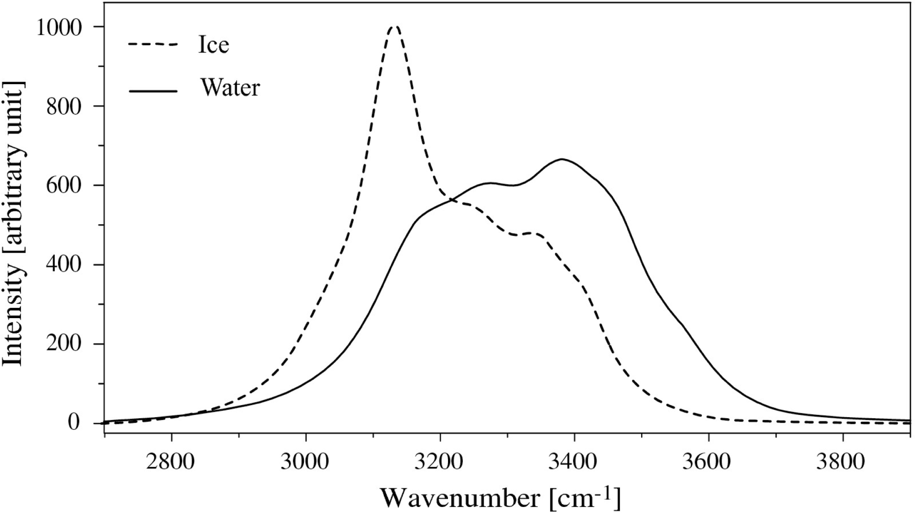
On Figure 1 is plotted the typical O – H stretching band recorded by RS in pure water in both solid and liquid phases. This broad band was widely investigated [3–5], and it is worth noting that the large change in its shape which occurs in both sides of the solid-liquid phase transition. This means that the lower part of the spectrum, which is related to fully H bonded atoms, is closely linked to the ordered solid phase, whereas the upper part which is ascribed by partly H−bonded and free O – H characterizes the liquid phase [6]. 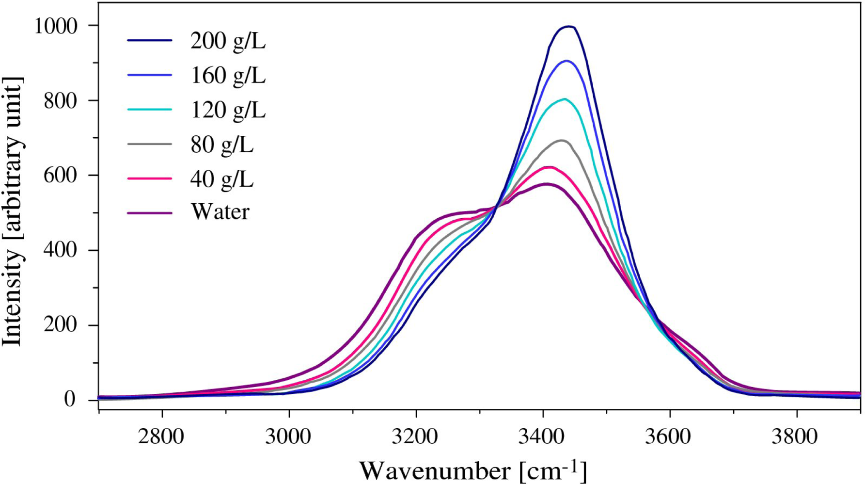Figure 2 shows the same part of the spectrum recorded in NaCl liquid solutions of various concentrations. This clearly reflects the own influence of NaCl introduction which affects the higher frequency part.

From these observations, a parameter S_$𝒟$ is defined as the ratio of the lower and upper parts of the O – H spectrum, which should be able to describe the temperature and concentration dependences of the solid-liquid phase transition. The order or disorder character of the transition in salted solutions can be reflected from the values of this quantity. We propose to use this parameter deduced from Raman scattering measurements to study the phase transition characteristics. According to the frequency range of the spectrum recorded in pure water (see Figure 2), the acquisition of the spectrum is made from 3000 to 3650 cm⁻¹. The O – H vibrations are then studied by comparing via S_$𝒟$ the integrated intensity J₁ (3000 → 3325 cm⁻¹) of the left side which is more sensitive to the temperature change and the integrated intensity J₂ (3325 → 3650 cm⁻¹) of the right side which is rather affected by the salt introduction. We therefore define the S_$𝒟$ parameter on Equation 1.

$$S_{𝒟}=\frac{J_2}{J_1}$$

(1)

The RS of O – H of water or brines is rather centered on 3325 cm⁻¹. This value was shown as the limit between the right and the left frequency parts of the O – H spectrum. We have checked that such a choice of the exact limit is not so important. In fact the analysis of physical mechanisms involved in the O – H spectrum is more complicated and usually the spectrum is deconvoluted into 4, 5 or 6 bands to interpret it. This is the subject of many controversies [3,7,8]. Here we choose an easier way by considering only two parts which are rather linked to one or another process. The results described below show that the results derived from the method described here are fairly good. Figure 3 shows the typical plot of S_$𝒟$ for pure water from −25 °C to 10 °C. This material could therefore be considered clearly as a standard, its freezing point identified at 0 °C. We point out the phase transition around the mid part of the two extrema.

This plot can be, as usually, fitted by means of a modified Boltzmann equation (Michel [9] and Polidori [10]) shown on Equation 2.

$$S_{𝒟}=(A_2+A_3 · T)+\frac{A_1-(A_2+A_3 · T)}{1+e^{(T-T_c)/\mathrm{\Delta }T}}$$

(2)

where T is the temperature of the medium, T_c the phase transition temperature, A₁ is the value of S_$𝒟$ when T ≪ T_c, A₂ is the y-intercept for the linear part of S_$𝒟$, obtained for T ≫ T_c, A₃ is the slope for T ≫ T_c, and ΔT is the specific slope at T = T_c. Thus defined, the parameters A₁ and A₂ characterize the order and disorder process within the phase transition since they correspond to ice and liquid water, respectively. Indeed A₃ is related to the thermal agitation, which is responsible for the breakdown of some hydrogen bonds, leading to an increasing disorder as the temperature raises.

As S_$𝒟$, A₁, A₂ and A₃ are quantities without units. We can notice that in case of A₃ = 0, typical Boltzmann curve is well obtained.

The fit curve on Figure 3 is obtained by the Levenberg-Marquart algorithm on the −25 → +10°C temperature range and the regression coefficient is R² = 0.998. It clearly indicates the good agreement between the experimental data and the calculated curve. From the results of the pure water, the suggested method was extended to study the phase transition characteristics of salted solutions of various concentrations.

3. Description of the probe and discussion of the results

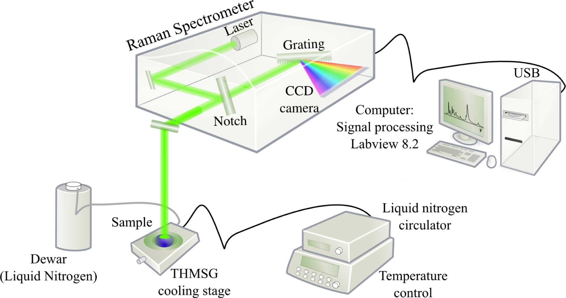
Figure 4 shows the sensor who mainly consists of a Raman spectrometer (including the laser, the notch filter and the CCD camera) and a computer for signal processing. The water sample is excited by an argon-ion laser at a wavelength of 514.5 nm, and with an output power of 25 mW. The Raman spectrum is measured in the backscattering configuration through a 50× long-working distance objective, located at about 8 mm of the top of the sample. The backscattered radiation is collected by a CCD camera of 1024 pixels.

The spectrometer with a spectral resolution of 2 cm⁻¹ is linked to the computer by an USB plug. The software was developed to do acquisitions, calibrations and process the signal to calculate S_$𝒟$, and to extract the phase transition temperature T_c. The value S_$𝒟$ is calculated by midpoint rule and developed on Equation 3.

$$S_{𝒟}=\frac{\sum _{i=326}^{650}\left[\frac{I(i)+I(i-1)}{2}\times \{n(i)-n(i-1)\}\right]}{\sum _{i=1}^{325}\left[\frac{I(i)+I(i-1)}{2}\times \{n(i)-n(i-1)\}\right]}$$

(3)

The main advantage of this simple method is the reduction of the noise influence. This calculus and the Levenberg-Marquart algorithm have been coded under LabVIEW 8.2.

In order to achieve to a simpler equation than Equation 2, calibrate of our sensor was performed by calculating the 5 parameters A₁, A₂, A₃, T_c et ΔT for any concentration. This technique also permits to save a significant calculation time. We perform several acquisitions of S_$𝒟$ for different concentrations in order to apply the modified Boltzmann regression.

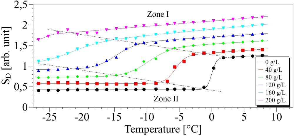
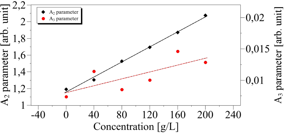
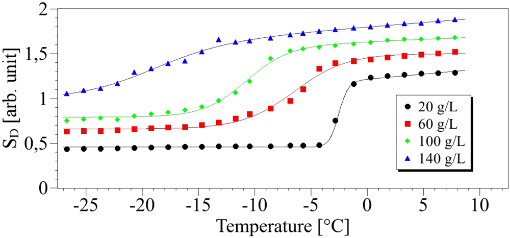
Figure 5 shows results of experimental data and associated fit for concentrations of salt from 0 to 200 g/L.

The values of A₂ and A₃ of Equation 2 can be determined from the zone I of Figure 5 and are deduced from a linear relationship: A₂ + A₃ · T which derives from equation 2 when T ≫ T_c. Both parameters are reported in Figure 6 as function of the concentration. We can observe on Figure 6, that a linear dependence of A₂ and A₃ on the concentration especially for A₂. The standard errors are s = 0.02 and s = 0.29 respectively and the correlation coefficients are respectively R² = 0.99 and R² = 0.57. These values for A₃ can be explained by the small slope of S_$𝒟$ leading to increasing uncertainties.

The relationship of A₂ and A₃ are then:

$$\begin{array}{l}{A}_2=1.16+4.50\times {10}^{-3} · \mathrm{C}\\ A_3=8.04\times {10}^{-3}+2.74\times {10}^{-5} · \mathrm{C}\end{array}$$

(4)

where C is the concentration. In the liquid phase, the behaviour of S_$𝒟$ can be linearly linked to the temperature as detailed Equation 5.

$$S_{𝒟}=1.16+(4.50\times {10}^{-3}+2.74\times {10}^{-5} · T) · \mathrm{C}+8.04\times {10}^{-3} · T$$

(5)

One should mention that temperature in pure liquid water could be therefore theoretically determined by Equation 5 with C = 0 g/L (see Equation 6).

$$T=124.3 · S_{𝒟}-144$$

(6)

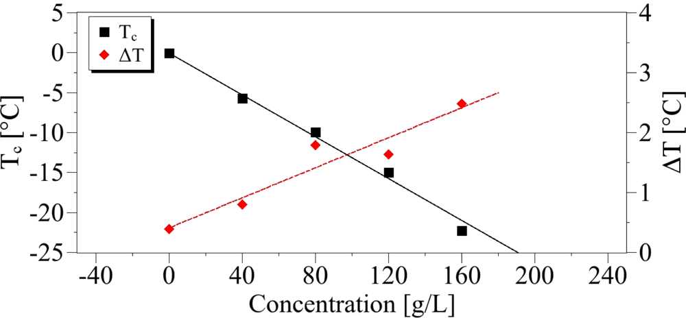
The liquid-solid phase transition zone was used to determine the T_c and ΔT parameters defined in Equation 2, and their concentration dependences.

We obtained:

$$\begin{array}{l}{T}_c=-0.131 · \mathrm{C}\\ \mathrm{\Delta }T=0.415+0.012 · \mathrm{C}\end{array}$$

(7)

The regression curve of the temperature T_c (figure 7) is provided with R² = 0.99 and s = 0.85, whereas for ΔT, the regression coefficient is R² = 0.91 and the standard error is s = 0.028. On these calculations, the value at the concentration 200 g/L was discarded since for large salt contents the solution is inhomogeneous so that the transition is not abrupt. Additionally this shows the limitation of our method in these cases. The introduction of increasing NaCl content induces changes of the phase transition characteristics revealed by the Raman probe. First, as expected, the increase in saline water concentration diminishes the freezing point, bringing it closer to −20 °C. Simultaneously the slope ΔT is growing with the salt content. 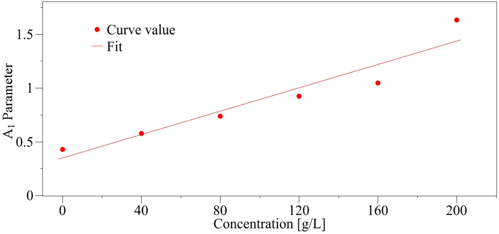In the high temperature (liquid phase), a disorder increase reflected by the parameter A₃ is as well observed with increasing concentration. Below the phase transition (solid phase), the plots of S_$𝒟$ are proportional to temperature (Zone II on Figure 5), so that of the parameter A₁ can be easily calculated and its dependence versus the concentration gives a straight line (cf. Figure 8).

The expression of parameter A₁ is thus written as:

$$A_1=3.48\times {10}^{-1}+5.43\times {10}^{-4} · \mathrm{C}$$

(8)

All values and the errors associated are summarized on

Table 1. Fitted parameters of curves of figure 5.

Concentration (g/L)	Parameters
	A1	A2	A3 (×10−3)	Tc (°C)	ΔT (°C)
0	0.430 ± 0.002	1.19 ± 0.01	7.4 ± 1.5	0.01 ± 0.002	0.39 ± 0.02
40	0.580 ± 0.003	1.300 ± 0.008	11.4 ± 1.3	−5.77 ± 0.06	0.80 ± 0.05
80	0.740 ± 0.004	1.530 ± 0.007	8.8 ± 0.2	−8.23 ± 0.12	1.79 ± 0.09
120	0.920 ± 0.006	1.690 ± 0.004	10.0 ± 0.7	−9.93 ± 0.10	1.63 ± 0.09
160	1.05 ± 0.02	1.870 ± 0.002	14.6 ± 0.4	−22.26 ± 0.27	2.48 ± 0.2
200	1.64 ± 0.08	2.080 ± 0.004	12.8 ± 0.4	−25.79 ± 0.95	0.56 ± 0.05

.

From them and from Equations 4, 7 and 8, we are able to simplify Equation 2 into Equation 9.

$$S_{𝒟}=(1.16+0.0045 · C)+(0.00804+0.000027 · C) · T+\frac{(-0.812+0.0009 · C)+(0.00804+0.000027 · C) · T)}{1+{\mathit{exp}}^{\frac{T-1.69+0.131 · C}{0.415+0.00125 · C}}}$$

(9)

The Raman probe of the phase transition was studied for eleven saline concentrations. The resulting plots for four concentrations are shown on Figure 9.

4. Conclusions

We propose to use a Raman sensor to probe the liquid-solid phase transitions in salted solutions, along with its thermodynamic characteristics. This new method can be deployed on several application fields where the knowledge of the phase transition is needed. We can mention: (1) both the water and ice phases on road during winter period, (2) frozen food control, as well as its production and its storage and (3) biodiversity studies where biological cycle depends on snow/ice/water phases. Our method is based on the rapid exploitation of the O – H Raman spectrum which is found to be strongly dependent on the temperature and salt concentration. For the ratio S_$𝒟$ of two parts of the spectrum, only their integrated scattered intensities are needed without any deconvolution. Parameters describing the phase transition are derived from the quantity S_$𝒟$ and their dependences on the concentration can be easily found.