Article

Modeling and Analysis of Energy Conservation Scheme Based on Duty Cycling in Wireless Ad Hoc Sensor Network

1
School of Electronic Engineering, Soongsil University, 511 Sangdo-dong, Dongjak-gu, Seoul, Korea
2
Department of Electrical and Computer Engineering, University of Waterloo, Waterloo, ON N2L 3G1, Canada
*
Author to whom correspondence should be addressed.
Sensors 2010, 10(6), 5569-5589; https://doi.org/10.3390/s100605569
Submission received: 5 February 2010 / Revised: 22 April 2010 / Accepted: 25 May 2010 / Published: 3 June 2010

Abstract

:
In sensor network, energy conservation is one of the most critical issues since sensor nodes should perform a sensing task for a long time (e.g., lasting a few years) but the battery of them cannot be replaced in most practical situations. For this purpose, numerous energy conservation schemes have been proposed and duty cycling scheme is considered the most suitable power conservation technique, where sensor nodes alternate between states having different levels of power consumption. In order to analyze the energy consumption of energy conservation scheme based on duty cycling, it is essential to obtain the probability of each state. In this paper, we analytically derive steady state probability of sensor node states, i.e., sleep, listen, and active states, based on traffic characteristics and timer values, i.e., sleep timer, listen timer, and active timer. The effect of traffic characteristics and timer values on the steady state probability and energy consumption is analyzed in detail. Our work can provide sensor network operators guideline for selecting appropriate timer values for efficient energy conservation. The analytical methodology developed in this paper can be extended to other energy conservation schemes based on duty cycling with different sensor node states, without much difficulty.

1. Introduction

Sensor network generally consists of multiple sensor nodes and a sink node, where sensor nodes monitor and measure physical information such as temperature, humidity, pressure, movement of any object, etc. [1, 2]. Sensed information is transferred from sensor nodes to a sink node via multi-hop routing and it is finally delivered to the central management system.
In sensor network, sensor nodes should perform a sensing task for a long time (e.g., lasting a few years) and the battery of them cannot be replaced in most practical situations. Therefore, energy conservation or power control is considered as one of the most critical issues in sensor network in order to guarantee a certain level of performance [3]. It is also widely accepted that energy consumption due to communication is much higher than that due to either sensing information or processing sensed information [4, 5]. Regarding energy consumption due to communication, just listening communication interface also consumes comparable power to receiving data and it is reported that the ratio of energy consumption among listening, receiving, and transmitting data is about 1, 1, and 1.5, respectively [5, 6]. Therefore, it is important to put communication interface of sensor nodes in low power sleep state when communication between neighbor sensor nodes is not required, in order to save energy [7].
In order to extend the lifetime of sensor nodes, numerous works have been carried out and most algorithms proposed in these works mainly use duty cycling, data-driven approaches, and mobility [4]. Duty cycling achieves energy conservation by putting unused communication interface of sensor nodes in low power sleep state as long as possible. Data-driven approaches reduce the number of sampled data by eliminating redundant data delivery to the sink node using correlation property between sampled data [8]. The energy consumption of sensor nodes can be reduced further if mobile nodes moving around sensor network can be used for data collection, and thus, sensor nodes just route their data to the mobile nodes via direct or limited multi-hop routing [9].
Out of these schemes, duty cycling scheme is considered the most suitable power conservation technique [4] and we only focus on energy conservation schemes based on duty cycling in this paper. In [4], the authors classify duty cycling as topology control and power management. In topology control, redundancy of sensor nodes is used and only a subset of sensor nodes are activated, while maintaining network connectivity, and the other sensor nodes are deactivated for power saving [1012]. Thus, it is important to decide which sensor nodes should be activated or deactivated in topology control.
Power management deals with activated sensor nodes and transitions between states having different levels of power consumption, such as sleep, listen, and active states, are controlled for efficient power conservation [1315]. In power management, sensor nodes initially stay in sleep state when communication is not required, by putting communication interface in the low power sleep state. In order to check any incoming data, a sensor node periodically wakes up at the expiration of sleep timer by moving into listen state and listens to the radio interface. In listen state, if there is no incoming data until the expiration of listen timer, it moves back to sleep state. Otherwise, its state changes to active state and communication with another sensor node is performed. In active state, if there is no further data to be transmitted or received until the expiration of active timer, after completing transmitting or receiving any data, it moves to sleep state again.
In duty cycling, since different states of sensor nodes have different levels of power consumption, it is essential to obtain the steady state probability of sensor node states in order to analyze the energy consumption [3]. Also, since state transitions are controlled by timer values, the effect of timer values and traffic characteristics on the steady state probability should be analyzed in detail, so that sensor network operators can select appropriate timer values of sensor nodes for efficient energy conservation. To the best of our knowledge, however, energy consumption in most previous works is analyzed via simulation, without deriving the steady state probability analytically. Furthermore, the effect of timer values on energy consumption has not been investigated analytically in detail. In this sense, our work is the first attempt to derive the steady state probability of sensor node states based on traffic characteristics and timer values and investigate the effect of traffic characteristics and timer values on energy consumption analytically. We note that since the analytical methodology developed in this paper is based on a general energy conservation scheme based on duty cycling, it can be extended to other energy conservation schemes based on duty cycling with different sensor node states, without much difficulty.
The remainder of this paper is organized as follows: Section 2 surveys related works on duty cycling. Section 3 develops analytical model for deriving steady state probability of sensor node states and obtains energy consumption. Numerical examples are presented in Section 4. Finally, Section 5 summarizes this work and presents further works.

2. Related Works

In this section, related works on energy conservation schemes based on duty cycling are surveyed. As mentioned in Introduction, duty cycling can be classified as topology control and power management. In addition, topology control is further divided into location driven protocol and connectivity driven protocol based on the criteria used to decide activation and deactivation of sensor nodes [4]. In location driven protocol, the location of sensor nodes is used as the criteria and geographical adaptive fidelity (GAF) [11] is a representative example of this protocol. In connectivity driven protocol, on the other hand, network connectivity is used as the criteria and Span [12] is one example of this protocol.
In GAF [11], sensor network is divided into grids, where any two sensor nodes located within adjacent grids can communicate with each other. In each grid, only one sensor node is active and other sensor nodes in the grid are in sleep state. There are three states in GAF, i.e., sleep, discovery, and active states. In sleep state, radio interface of a sensor node is put into sleep state and the sensor node moves into discovery state at the expiration of sleep timer. In discovery state, the sensor node exchanges discovery messages with other sensor nodes within the same grid. If the sensor node receives a discovery message from a sensor node with higher rank, i.e., higher residual energy, within discovery timer, it moves back to sleep state. Otherwise, it moves to active state. In active state, if the sensor node receives a discovery message from a sensor node with higher rank within active timer, it enters into sleep state. Otherwise, it moves back to discovery state at the expiration of active timer.
Span [12] is a distributed backbone selection protocol and adaptively elects coordinators in sensor network. The coordinators perform multi-hop routing for other sleeping sensor nodes by staying awake. Sensor nodes in sleep state periodically wake up and check whether to sleep or stay awake as a coordinator using coordinator eligibility rule which is based on the battery level and the number of neighbor sensor nodes. In coordinator eligibility rule, if two neighbor sensor nodes of a non-coordinator sensor node cannot reach each other, either directly or via one or two coordinators, the non-coordinator sensor node becomes a coordinator sensor node. In order to avoid the situation that multiple sensor nodes become a coordinator at the same time, a random back off delay is used before taking a coordinator role. Each coordinator periodically checks if it can withdraw a coordinator role by checking if every pair of sensor nodes of its neighbor sensor nodes can communicate, either directly or via one or two coordinators.
In power management, activated sensor nodes alternate between sleep, listen, and active states, based on traffic characteristics, without depending on topology or connectivity information. The power management scheme is further divided into sleep/wakeup protocol which is independent on medium access control (MAC) protocol and MAC protocol with low duty cycle, where sleep/wakeup is tightly coupled with MAC protocol [4]. In this paper, we only focus on sleep/wakeup protocol because it can be used with any MAC protocol. Basic energy conservation algorithm (BECA)[13] and sparse topology and energy management (STEM) [14] belong to this protocol.
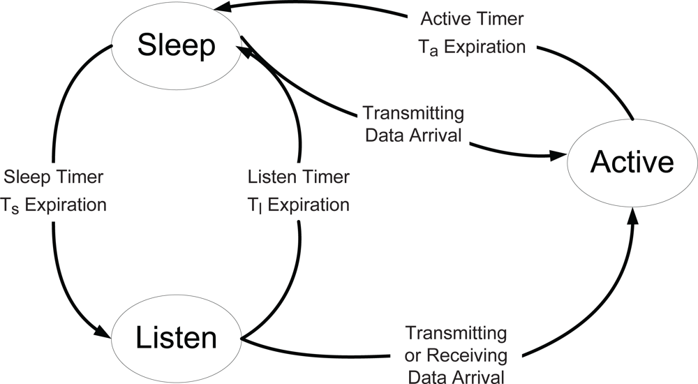
In BECA [13], sensor nodes stay in sleep state initially when communication is not required, by putting the communication interface in the low power sleep state. Each sensor node periodically wakes up for every sleep timer, Ts, by moving into listen state and listens any incoming data to the sensor node during listen timer, Tl. In listen state, if there is no incoming data until the expiration of the listen timer, it moves back to sleep state again. Otherwise, its state changes to active state and it communicates with another sensor node. In active state, if there is no further data to be transmitted or received until the expiration of active timer, Ta, after completing transmitting or receiving any data, it moves to sleep state again. Figure 1 shows state transition model of BECA.
In STEM [14], all sensor nodes wake up simultaneously for every Twakeup and remain in active state for active time. Then, they move to sleep state at the same time until the next wakeup time. In STEM, low duty cycle, i.e., high energy efficiency, is possible by adjusting active time much smaller than wakeup time. The STEM has the problem of high probability of collisions due to simultaneous wakeup and thus, staggered wakeup pattern (SWP) [15] has been proposed to solve this problem by waking up sensor nodes at different times based on the different levels of routing tree.

3. Modeling and Analysis of Sensor Node State Transition Model

In this paper, we develop an analytical methodology for deriving steady state probability of sensor node states of BECA as an example. We note that the analytical methodology developed for BECA can be extended to other energy conservation schemes based on duty cycling with different sensor node states, without much difficulty.

3.1. Modeling of Sensor Node State Transition

Figure 2 shows a modified state transition model of BECA, where active state in original state transition model of BECA is divided into four sub-states; active-transmit, active-receive, active-forward, and active-idle states, for ease of mathematical derivation. In active-transmit state, a sensor node transmits its locally generated sensing data to a sink node. In active-forward state, on the other hand, a sensor node relays sensing data from other sensor nodes to neighbor sensor nodes. In active-receive state, a sensor node receives sensing data from other sensor nodes. In active-idle state, the sensor node does not receive or transmit any sensing data, and if there is no further data to be transmitted or received until the expiration of active timer, it moves to sleep state. We note that we differentiate active-forward state from active-transmit state because traffic characteristic for a sensor node’s locally generated sensing data traffic is different from aggregated sensing data generated by other sensor nodes, and thus, we need to consider them separately for an accurate modeling [16].

3.2. Derivation of Steady State Probability

For mathematical derivation, we need to assume traffic model of sensor networks, which depends on the data reporting process of considered sensor network applications, i.e., event-driven, time-driven, and query-driven [17, 18]. In event-driven case, data are generated when an event occurs. In time-driven case, data are generated periodically. In query-driven case, data are generated by the request of a sink node when needed. In this paper, we mainly focus on event-driven case and it is proved that the data generation at an individual sensor node follows a Poisson process, based on the assumptions that the event is uniformly distributed in sensor networks and every event is independent of other events [17]. Regarding the service time of data packet, we use an exponential distribution model for more general consideration of service time, although simple constant bit rate (CBR) model is commonly used. The use of Poisson and exponential distributions allows us to develop a tractable analytical model for deriving steady state probability of sensor node states. The developed model based on Poisson and exponential distributions can be easily extended to other cases with different traffic model.
Based on the above discussions, we have made the following assumptions regarding the density functions of random variables:
  • Transmitting, receiving, and forwarding data packets at a sensor node occur according to a Poisson process with parameters λt, λr, and λf, respectively;
  • The time duration that a sensor node remains in active-transmit, active-receive, and active-forward states follows an exponential distribution with a mean value of 1 / μt, 1 / μr, and 1 / μf ;
  • The values of sleep timer, listen timer, and active timer are assumed as constant and they are denoted by Ts, Tl, and Ta, respectively.
We denote sleep, listen, active-transmit, active-receive, active-forward, and active-idle states as states 1, 2, 3, 4, 5, and 6, respectively, for notational convenience. Since the residence times of a sensor node in sleep, listen, and active-idle states do not follow an exponential distribution, the sensor node state transition behavior is analyzed using a semi-Markov process approach [19].
The steady state probability of each sensor node state can be obtained as [19]:
P k = π k t k ¯ i = 1 6 π i t i ¯ ,               k = 1 , 2 , 3 , 4 , 5 ,   and   6
where πk denotes the stationary probability of state k and t k ¯ is the mean residence time of the sensor node in state k. The stationary probability is obtained by solving the following balancing equations [19]:
π j = k = 1 6 π k P kj ,   j = 1 , 2 , 3 , 4 , 5 ,   and   6
1 = k = 1 6 π k  
where Pkj represents the state transition probability from state k to state j. The state transition probability matrix P = [pkj] of the state transition model is given by:
P = ( 0 P 12 P 13 0 0 0 P 21 0 P 23 P 24 P 25 0 0 0 0 0 0 P 36 0 0 0 0 0 P 46 0 0 0 0 0 P 56 P 61 0 P 63 P 64 P 65 0 )
Then, stationary probabilities can be solved as:
π 1 = 1 D
π 2 = P 12 π 1 = P 12 D
π 3 = P 61 P 13 + P 61 P 12 P 23 + P 63 ( 1 P 12 P 21 ) P 61 π 1 = P 61 P 13 + P 61 P 12 P 23 + P 63 ( 1 P 12 P 21 ) P 61 D
π 4 = P 61 P 12 P 24 + P 64 ( 1 P 12 P 21 ) P 61 π 1 = P 61 P 12 P 24 + P 64 ( 1 P 12 P 21 ) P 61 D
π 5 = P 61 P 12 P 25 + P 65 ( 1 P 12 P 21 ) P 61 π 1 = P 61 P 12 P 25 + P 65 ( 1 P 12 P 21 ) P 61 D
π 6 = 1 P 12 P 21 P 61 π 1 = 1 P 12 P 21 P 61 D
where D is obtained by:
D = 1 + P 12 ( 1 + P 23 + P 24 + P 25 ) + P 13 + 1 + P 63 + P 64 + P 65 P 12 P 21 ( 1 + P 63 + P 64 + P 65 ) P 61
State transition probability Pkj can be derived based on the distribution of time from states k to j, Tkj. Exit from the sleep state is caused by any of the following events:
  • Sleep timer expiration (T12);
  • A transmitting data packet arrival (T13).
Then, the state transition probabilities P12 and P13 are obtained as:
P 12 = 0 f T 12 ( t ) Pr ( T 13 > t ) dt = 0 δ ( t T s ) 0 λ t   e λ t   u dudt = 0 δ ( t T s ) e λ t   t dt = e λ t   T s
P 13 = 1 P 12 = 1 e λ t T s
Exit from the listen state is caused by any of the following events:
  • Listen timer expiration (T21);
  • A transmitting data packet arrival (T23);
  • A receiving data packet arrival (T24);
  • A forwarding data packet arrival (T25).
Then, the state transition probability P21 is obtained as:
P 21 = 0 f T 21 ( t ) Pr ( T 23 > t ) Pr ( T 24 > t ) Pr ( T 25 > t ) dt = 0 δ ( t T l ) t λ t e λ t u du t λ r e λ r u du t λ f e λ f   u dudt = 0 δ ( t T l ) e λ t t e λ r t e λ f   t dt = e ( λ t + λ r + λ f ) T t
Similarly, the state transition probabilities P23, P24, and P25 are obtained as:
P 23 = 0 f T 23 ( t ) Pr ( T 21 > t ) Pr ( T 24 > t ) Pr ( T 25 > t ) dt = λ t λ t + λ r + λ f ( 1 e ( λ t + λ r + λ f ) T l )
P 24 = 0 f T 24 ( t ) Pr ( T 21 > t ) Pr ( T 23 > t ) Pr ( T 25 > t ) dt = λ r λ t + λ r + λ f ( 1 e ( λ t + λ r + λ f ) T l )
P 25 = 0 f T 25 ( t ) Pr ( T 21 > t ) Pr ( T 23 > t ) Pr ( T 24 > t ) dt = λ f λ t + λ r + λ f ( 1 e ( λ t + λ r + λ f ) T l )
In active-transmit, active-receive, and active-forward states, exit from these states are caused by the service completion of transmitting, receiving, and forwarding data packets, respectively, and the state transition probabilities P36, P46, and P56 are simply obtained as:
P 36 = P 46 = P 56 = 1
Exit from the active-idle state is caused by any of the following events:
  • Active timer expiration (T61);
  • A transmitting data packet arrival (T63);
  • A receiving data packet arrival (T64);
  • A forwarding data packet arrival (T65).
Then, the state transition probability P61 is obtained as:
P 61 = 0 f T 61 ( t ) Pr ( T 63 > t ) Pr ( T 64 > t ) Pr ( T 65 > t ) dt = 0 δ ( t T a ) t λ t e λ t u du t λ r e λ r u du t λ f e λ f   u dudt = 0 δ ( t T a ) e λ t t e λ r t e λ f   t dt = e ( λ t + λ r + λ f ) T a
Similarly, the state transition probabilities P63, P64, and P65 are obtained as:
P 63 = 0 f T 63 ( t ) Pr ( T 61 > t ) Pr ( T 64 > t ) Pr ( T 65 > t ) dt = λ t λ t + λ r + λ f ( 1 e ( λ t + λ r + λ f ) T a )
P 64 = 0 f T 64 ( t ) Pr ( T 61 > t ) Pr ( T 63 > t ) Pr ( T 65 > t ) dt = λ r λ t + λ r + λ f ( 1 e ( λ t + λ r + λ f ) T a )
P 65 = 0 f T 65 ( t ) Pr ( T 61 > t ) Pr ( T 63 > t ) Pr ( T 64 > t ) dt = λ f λ t + λ r + λ f ( 1 e ( λ t + λ r + λ f ) T a )
Now, we have derived all the state transition probabilities, and the mean residence time of the sensor node in each state is calculated. The mean residence time in the sleep state is derived as:
t 1 ¯ = E [ t 1 ] = E [ min { T 12 ,   T 13 } ] = 0 Pr ( min { T 12 ,   T 13 } > t ) dt = 0 Pr ( T 12 > t ) Pr ( T 13 > t ) dt = 0 U [ T s t ] e λ t t dt = 0 T s e λ t t dt = 1 e λ t T s λ t
The mean residence time in the listen state is similarly derived as:
t 2 ¯ = E [ t 2 ] = E [ min { T 21 ,   T 23 , T 24 , T 25 } ] = 0 Pr ( min { T 21 ,   T 23 , T 24 , T 25 } > t ) dt = 0 Pr ( T 21 > t ) Pr ( T 23 > t )   Pr ( T 24 > t )   Pr ( T 25 > t ) dt = 0 e λ t t Pr ( T 21 > t ) Pr ( T 24 > t ) Pr ( T 25 > t ) dt = 1 λ t P 23 = 1 λ t + λ r + λ f ( 1 e ( λ t + λ r + λ f ) T l )
The mean residence time in the active-transmit state is derived as:
t 3 ¯ = E [ t 3 ] = E [ min { T 36 } ] = 0 Pr ( min { T 36 } > t ) dt = 0 e μ t t dt = 1 μ t
Likewise, the mean residence time in the active-receive and active-forward is derived as:
t 4 ¯ = E [ T 4 ] = E [ min { T 46 } ] = 0 Pr ( min { T 46 } > t ) dt = 0 e μ t t dt = 1 μ r
t 5 ¯ = E [ t 4 ] = E [ min { T 46 } ] = 0 Pr ( min { T 46 } > t ) dt = 0 e μ t t dt = 1 μ f
The mean residence time in the active-idle state is derived as:
t 6 ¯ = E [ t 6 ] = E [ min { T 61 ,   T 63 , T 64 , T 65 } ] = 0 Pr ( min { T 61 ,   T 63 , T 64 , T 65 } > t ) dt = 0 Pr ( T 61 > t ) Pr ( T 63 > t )   Pr ( T 64 > t )   Pr ( T 65 > t ) dt = 0 e λ t t Pr ( T 61 > t ) Pr ( T 64 > t ) Pr ( T 65 > t ) dt = 1 λ t P 63 = 1 λ t + λ r + λ f ( 1 e ( λ t + λ r + λ f ) T a )
Based on the values of πk and t k ¯ obtained from Equations (4)(9) and Equations (22)(27), respectively, we can finally derive the steady state probability of each sensor node state using Equation (1) [19]. Now, we can obtain the energy consumption of a sensor node per unit time by using the steady state probability as:
E = k = 1 6 ψ k P k
where ψk is the power consumption in state k.R

4. Numerical Examples

4.1. Parameters Setting

In this section, numerical examples are presented in order to show the effect of various parameters on the steady state probability and energy consumption. In sensor network, since sensor nodes transmit locally generated sensing data to a sink node and the locally generated data traffic from sensor nodes contributes to forwarding data traffic of a sensor node, we relate local transmitting data traffic and forwarding data traffic of a sensor node by λf = wfλt, where wf is the weighting factor for forwarding data traffic to local transmitting data traffic and it is proportional to the number of sensor nodes in sensor network. Also, since forwarding traffic should be received first before forwarding [16], the relationship λr = λf is assumed. The relationship 1/μt = 1/μr = 1/μf is also assumed since each sensor node normally generates sensing data with the same size. Based on these relationships, we define activity of a sensor node as follows:
ρ = λ t + λ r + λ f μ t = ( 1 + 2 w f ) λ t μ t
The default parameters for timers and traffic characteristic are given by Table 1. Parts of the parameters in Table 1 vary in the following numerical examples in order to analyze the effect of the parameters on the performance. Power consumption in each state is assumed, as the ones depicted in Table 2, based on the energy model described in [6, 11, 12].

4.2. Effect of Sleep Timer, Ts

Figure 3 shows the effect of sleep timer on the steady state probability of sleep, listen, and active states. We note that instead of showing the probabilities of four sub-states; active-transmit, active-receive, active-forward, and active-idle states which have a very similar pattern, we just show the probability of active state collectively, in order to avoid confusion and strengthen the result. To validate the analytical methodology developed in this paper, we conducted a discrete-event simulation for steady state probabilities, using C++ language. The simulation results were obtained by running 104 h of simulation time after 103 hours of warm-up time. From the results, it is shown that the validity of the proposed analytical model is proved since analysis results are well matched with simulation results. As the value of sleep timer increases, the probability of sleep state decreases, since it is more likely that a sensor node stays in sleep state more for higher value of sleep timer. On the other hand, the probabilities of listen state and active state decrease, because the chance of staying in either listen state or active state decreases due to increased probability of sleep timer.
Figure 4 shows the effect of sleep timer on the energy consumption for varying activity, where the values of λt, λr, and λf are changed with 1 μ t = 1 μ r = 1 μ f = 1 3600 h. We note that simulation results only for steady state probabilities are presented but those for energy consumption are not presented in this paper since energy consumption is just a weighted sum of steady state probabilities, and thus, the validity of the analytical model for energy consumption is proved by just showing that for steady state probabilities. As can be expected from the result in Figure 3, the energy consumption decreases as the value of sleep timer increases, since the effect of sleep state becomes dominant, which has low power consumption. For a fixed value of sleep timer, energy consumption increases as the activity increases due to more transitions to active state with higher power consumption. We note that although the energy consumption decreases as the value of sleep timer increases, this also increases wakeup delay from sleep state to listen state. Therefore, an appropriate selection of sleep timer is needed to tradeoff between power consumption and wakeup delay.
Figure 5 shows the effect of sleep timer on the energy consumption for varying service time, where the value of activity is fixed as 0.1. Although the value of activity is the same, smaller service time, i.e., higher data arrival, results in more state changes into active state. Therefore, the energy consumption increases as the service time for transmitting, receiving, or forwarding data decreases. This is because although the total service time for either transmitting, receiving, or forwarding data is the same for the same activity, the sensor node with higher data arrival rate has higher probability of active state, since the sensor node stays in active state additionally until the expiration of active timer, where the number of the expirations of active timer is higher for higher rate of data arrival.

4.3. Effect of Listen Timer, Tl

Figure 6 shows the effect of listen timer on the steady state probability using both analysis and simulation. Similar to Figure 3, analysis results are well matched with simulation results. The probability of sleep state decreases, as the value of listen timer increases, since it is more likely that a sensor node stays in listen state more for higher value of listen timer, which is evident from the definition of listen timer. The probability of active state increases since it has more chances to make transition from listen state to active state due to data arrival, as the value of listen timer increases.
Figure 7 shows the effect of listen timer on the energy consumption for varying activity, where the values of λt, λr, and λf are changed with 1 μ t = 1 μ r = 1 μ f = 1 3600 h. As can be expected from the result in Figure 6, the energy consumption increases as the value of listen timer increases, since the probabilities of listen and active states, which have higher power consumption, increase. For a fixed value of listen timer, energy consumption increases as the activity increases due to more transitions into active state with higher power consumption. We note that although smaller value of listen timer is better, from the aspect of energy consumption, the smaller value of listen timer results in more transitions into sleep state. Since more transitions into sleep state result in higher wakeup delay, an appropriate selection of listen timer is needed to tradeoff between power consumption and wakeup delay.
Figure 8 shows the effect of listen timer on the energy consumption for varying service time, where the value of activity is fixed to 0.1. Although the value of activity is the same, the energy consumption increases as the service time for transmitting, receiving, or forwarding data decreases due to the similar rationale, as in Figure 5.

4.4. Effect of Active Timer, Ta

Figure 9 shows the effect of active timer on the steady state probability using both analysis and simulation. Similar to previous figures on steady state probabilities, analysis results are well matched with simulation results, as well. As can be expected, the probability of active state increases, as the value of active timer increases. On the other hand, the probability of sleep and listen states decreases, as the value of active timer increases. This is due to the fact that higher value of active timer results in less transitions to sleep state, and thus, the transition from sleep state to listen state is also less likely to occur.
Figure 10 shows the effect of active timer on the energy consumption for varying activity, where the values of λt, λr, and λf are changed with 1 μ t = 1 μ r = 1 μ f = 1 3,600 h. Since the probability of active state increases as the value of active timer increases, the energy consumption also increases since active state has more power consumption. For a fixed value of active timer, energy consumption generally increases as the activity increases, due to more transitions into active state with higher power consumption. On the other hand, for very small values of active timer, energy consumption decreases, even though the activity increases, because more transitions into active state due to higher activity also results in more transitions into listen state with very low power consumption from active state, after the fast expiration of small active timer.
Figure 11 shows the effect of active timer on the energy consumption for varying service time, where the value of activity is fixed as 0.1. Although the value of activity is the same, the energy consumption generally increases as the service time for transmitting, receiving, or forwarding data decreases due to the similar rationale, as in Figure 8. On the other hand, for very small values of active timer, energy consumption decreases as the service time increases, due to the similar rationale, as in Figure 10.

4.5. Effect of λt

Figure 12 shows the effect of λt on the steady state probability for λf = λr = 10/h using both analysis and simulation. Similar to previous figures on steady state probabilities, analysis results are well matched with simulation results, too. The steady state probability of active state sharply increases, as the value of λt increases, which also increases the values of λr and λf. On the other hand, the steady state probabilities of both sleep and listen states decrease, as the value of λt increases, due to more transitions to active state from these states.
Figure 13 shows the effect of λt on the energy consumption for varying service time, where the value of activity increases as the service time increases. As can be expected from Figure 12, the energy consumption also sharply increases, as the value of λt increases, with the dominant effect of active state having higher power consumption. For a fixed value of λt, power consumption also increases as the service time increases due to higher activity.

5. Conclusions and Further Works

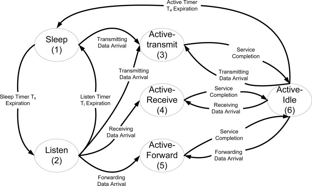
In this paper, we developed an analytical methodology of state transition model of an energy conservation scheme based on duty cycling and derive both steady state probability of sensor node states and energy consumption analytically based on traffic characteristic and timer values. Then, the effects of sleep timer, listen timer, active timer, and traffic characteristics on the steady state probability and energy consumption have been analyzed.
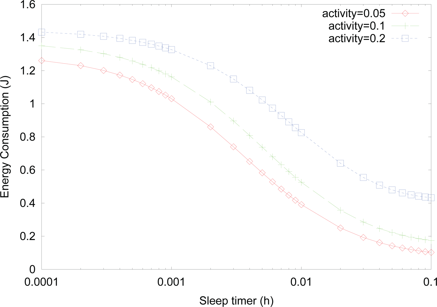
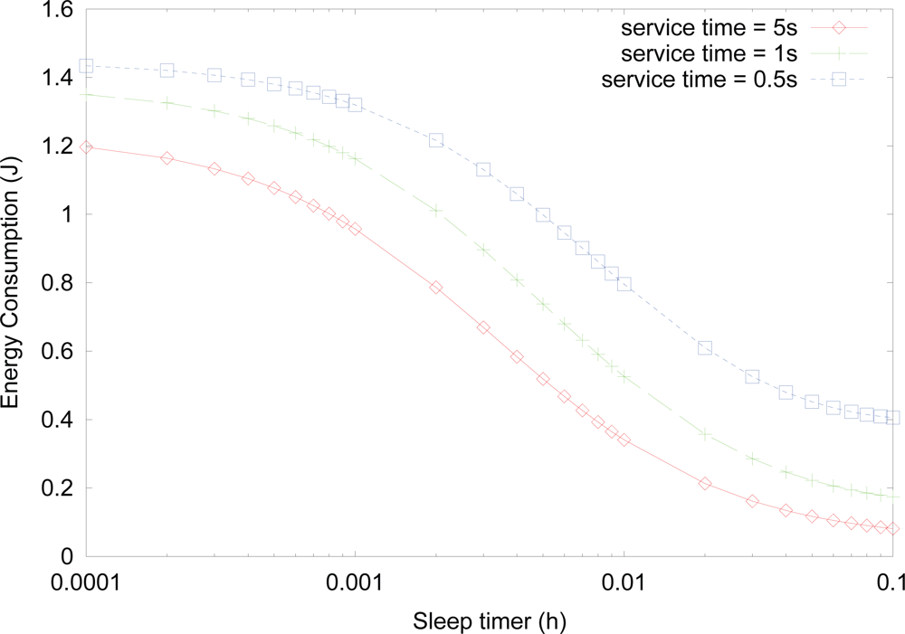
From the numerical examples, it can be concluded that the steady state probability and thus, resulting energy consumption are very sensitive to the change of timer values and traffic characteristic, and thus, an appropriate selection of timer values taking into account of traffic characteristics is very important for efficient power conservation. The result of this paper can provide sensor network operators guideline for selecting appropriate timer values for efficient energy conservation, depending on traffic characteristic. We note that since the analytical methodology developed in this paper is based on a general energy conservation scheme based on duty cycling, it can be extended to other energy conservation schemes based on duty cycling with different sensor node states, without difficulty.
As further works, the effect of timer values and traffic characteristics on the other performance measures, such as the delay of data delivery and the number of retransmissions for successful routing will be analyzed for more thorough analysis of an energy conservation scheme based on duty cycling, using the analytical model developed in this paper. The extension of the proposed analytical model for system optimization or design of a new duty cycling scheme, such as traffic-aware duty cycling scheme based on dynamic adjustments of optimal timer values for varying traffic environments, will be studied in further works too.

Acknowledgments

This research is supported by the ubiquitous Computing and Network (UCN) Project, the Ministry of Knowledge and Economy(MKE) Knowledge and Economy Frontier R&D Program in Korea as a result of UCNs subproject 10C2-C1-20S.

References

  1. Akyildiz, I.; Su, W.; Sankarasubramaniam, Y.; Cayirci, E. A survey on sensor networks. IEEE Commun. Mag 2002, 40, 102–114. [Google Scholar]
  2. Yick, J.; Mukherjee, B.; Ghosal, D. Wireless sensor network survey. Elsevier Comput. Netw 2008, 52, 2292–2330. [Google Scholar]
  3. Pantazis, N.A.; Vergados, D.D. A Survey on Power Control Issues in Wireless Sensor Networks. IEEE Commun. Surv. Tutorials 2007, 9, 86–107. [Google Scholar]
  4. Anastasi, G.; Conti, M.; Francesco, M.D.; Passarella, A. Energy conservation in wireless sensor networks: A survey. ElsevierAd Hoc Networks 2009, 7, 537–568. [Google Scholar]
  5. Savvides, A.; Han, C.C.; Srivastava, M. Dynamic fine-grained localization in ad hoc networks of sensors. Proceedings of the ACM SIGMOBILE Annual International Conference on Mobile Computing and Networking, Rome, Italy, July 16–21, 2001; pp. 166–179.
  6. Stemm, M.; Katz, R.H. Measuring and reducing energy consumption of network interfaces in hand-held devices. IEICE Trans. Commun 1997, E80-B, 1125–1131. [Google Scholar]
  7. Jones, C.E.; Sivalingam, K.M.; Agrawal, P.; Chen, J.C. A survey of energy efficient network protocols for wireless networks. Wirel. Netw 2001, 7, 343–358. [Google Scholar]
  8. Vuran, M.C.; Akan, O.B.; Akyildiz, I.F. Spatio-temporal correlation: theory and applications for wireless sensor networks. Elsevier Comput. Netw 2004, 45, 245–261. [Google Scholar]
  9. Chakrbarti, A.; Sabharwal, B.; Zazhang, B. Using predictable observer mobility for power efficient design of sensor networks. Proceedings of the 2nd International Workshop on Information Processing in Sensor Networks, Palo Alto, CA, USA, April 22–23, 2003; pp. 129–145.
  10. Santi, P. Topology control in wireless ad hoc and sensor network. ACM Comput. Surv 2005, 37, 164–194. [Google Scholar]
  11. Xu, Y.; Heidemann, J.; Estrin, D. Geography-informed energy conservation for ad hoc routing. Proceedings of the ACM SIGMOBILE Annual International Conference on Mobile Computing and Networking, Rome, Italy, July 16–21, 2001; pp. 70–84.
  12. Chen, B.; Jamieson, K.; Balakrishnan, H.; Morris, R. Span: An energy-efficient coordination algorithm for topology maintenance in ad hoc wireless networks. Wirel. Netw 2002, 8, 85–96. [Google Scholar]
  13. Xu, Y.; Heidemann, J.; Estrin, D. Adaptive Energy-conservation Routing for Multi-hop Ad Hoc Networks; Technical Report 527; USC/Informaton Sciences Institute: Marina del Rey, CA, USA, 2000. [Google Scholar]
  14. Schugers, C.; Tsiatsis, V.; Srivastava, M.B. STEM: topology management for energy efficient sensor networks. Proceedings of the IEEE Aerospace Conference, Big Sky, MT, USA, March 9–16, 2002.
  15. Keshavarzian, A.; Lee, H.; Venkatraman, L. Wakeup scheduling in wireless sensor networks. Proceedings of the ACM International Symposium on Mobile Ad Hoc Networking and Computing, Florence, Italy, May 22–25, 2006; pp. 322–333.
  16. Gao, Q.; Blow, K.J.; Holding, D.J.; Marshall, I. Analysis of energy conservation in sensor networks. Wirel. Netw 2005, 11, 787–794. [Google Scholar]
  17. Rai, V.; Mahapatra, R.N. Lifetime modeling of a sensor network. Proceedings of the Conference on Design, Automation and Test in Europte, Washington, DC, USA, March 2005; pp. 202–203.
  18. Noori, M.; Ardakani, M. A probability model for lifetime of event-driven wireless sensor networks. Proceedings of the 5th Annual IEEE Communications Society Conference on Sensor, Mesh and Ad Hoc Communications and Networks, San Francisco, CA, USA, June 16–20, 2008; pp. 269–277.
  19. Ross, S.M. Stochastic Processes; John Wiley & Sons: Hoboken, NJ, USA, 1996. [Google Scholar]
Figure 1. State transition model of BECA.
Sensors 10 05569f1
Figure 2. A modified state transition model of BECA.
Sensors 10 05569f2
Figure 3. Effect of sleep timer on the steady state probability.
Sensors 10 05569f3
Figure 4. Effect of sleep timer on the energy consumption for varying activity.
Sensors 10 05569f4
Figure 5. Effect of sleep timer on the energy consumption for varying service time.
Sensors 10 05569f5
Figure 6. Effect of listen timer on the steady state probability.
Sensors 10 05569f6
Figure 7. Effect of listen timer on the energy consumption for varying activity.
Sensors 10 05569f7
Figure 8. Effect of listen timer on the energy consumption for varying service time.
Sensors 10 05569f8
Figure 9. Effect of active timer on the steady state probability.
Sensors 10 05569f9
Figure 10. Effect of active timer on the energy consumption for varying activity.
Sensors 10 05569f10
Figure 11. Effect of active timer on the energy consumption for varying service time.
Sensors 10 05569f11
Figure 12. Effect of λt on the steady state probability.
Sensors 10 05569f12
Figure 13. Effect of λt on the energy consumption.
Sensors 10 05569f13
Table 1. Parameter values for timers and traffic characteristic.
ParameterValue
Ts 10 3600 h
Tl 10 3600 h
Ta 10 3600 h
ρ0.1
wf10
1 μ t 10 3600 h
1 μ r 10 3600 h
1 μ f 10 3600 h
λt 3600 210 / h
λr 3600 21 / h
λf 3600 21 / h
Table 2. Parameter values for power consumption.
ParameterValue
ψ10.025 W
ψ21.155 W
ψ31.6 W
ψ41.2 W
ψ51.6 W
ψ61.5 W

