Field Calibrations of Soil Moisture Sensors in a Forested Watershed

Abstract
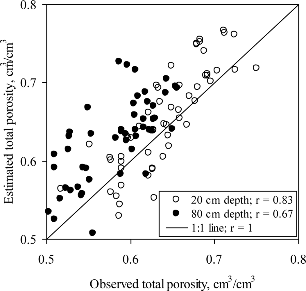
: Spatially variable soil properties influence the performance of soil water content monitoring sensors. The objectives of this research were to: (i) study the spatial variability of bulk density (ρb), total porosity (θt), clay content (CC), electrical conductivity (EC), and pH in the upper Mākaha Valley watershed soils; (ii) explore the effect of variations in ρb and θt on soil water content dynamics, and (iii) establish field calibration equations for EC-20 (Decagon Devices, Inc), ML2x (Delta-T-Devices), and SM200 (Delta-T-Devices) sensors to mitigate the effect of soil spatial variability on their performance. The studied soil properties except pH varied significantly (P < 0.05) across the soil water content monitoring depths (20 and 80 cm) and six locations. There was a linear positive and a linear inverse correlation between the soil water content at sampling and ρb, and between the soil water content at sampling and θt, respectively. Values of laboratory measured actual θt correlated (r = 0.75) with those estimated from the relationship θt = 1 − ρb/ρs, where ρs is the particle density. Variations in the studied soil properties affected the performance of the default equations of the three tested sensors; they showed substantial under-estimations of the actual water content. The individual and the watershed-scale field calibrations were more accurate than their corresponding default calibrations. In conclusion, the sensors used in this study need site-specific calibrations in order to mitigate the effects of varying properties of the highly weathered tropical soils.1. Introduction
Non-agricultural forested lands exhibit spatially variable soil water content as a function of soil basic properties [1], land cover [2], and topography [3]. Soil water content varies across a soil profile due to changes in ρb, θt, and CC [4,5]. Surface soil layers of forested watersheds are subject to higher soil water content dynamics due to evapotranspiration and rainfall; deep soil profiles have higher water content due to uniform conditions.
Accurate measurement of soil water content is important for water balance and hydrologic flux calculations, rainfall-runoff-infiltration models, ground truthing of remote sensing data, irrigation scheduling, water allocation calculations, and evaluation of potential drought impacts on stream flow [6]. Reliable measurement of soil water content with water sensors has been challenging in forested lands due to spatially variable soil physical and hydrological properties [6]. Variations in ρb have greater effects on sensor readings than those caused by CC or organic matter content [7].
Direct measurements of soil water content by the thermo-gravimetric method is more accurate than any other indirect method; however, this method is labor intensive, time consuming, destructive, and discrete for repetitive measurements. Indirect techniques of soil water content measurement (e.g., single- and multi-capacitance soil water content monitoring systems) overcome these disadvantages of the thermo-gravimetric method; in addition, they enable automate real-time spatially-distributed data collection [8,9]. Such techniques have been used for real-time monitoring of soil water content at different scales, i.e., greenhouse, field plots, watersheds subject to different agricultural management practices. Installation of theses sensors begins with a careful selection of monitoring locations, which are conceptually subdivided into macro- and micro-zones [8]. Macro-zone refers to the selection of one or several locations in a watershed or in an agricultural field characterized by dominant topography, soil type, vegetation, and management practices. On the other hand, micro-zone selection aims at determining the position of the sensor in relation to individual points/locations, soil depths (shallow vs. deep) or irrigation delivery points (drip or sprinkler emitter).
The single soil water content monitoring sensors EC-20 [10], ML2x [11], and SM200 [11] have been used in agricultural and non-agricultural settings. These sensors were calibrated under different soil and environmental conditions [12,13]. Czarnomski et al. [14] compared the accuracy and precision of the EC-20 with those of a TDR under field and laboratory conditions. They found that the default calibration equation of EC-20 underestimated water content by up to 0.12 cm3 cm−3 and that EC-20 wasn’t sensitive to ρb; they also concluded that the EC-20 data were more consistent than those of TDR. Logsdon and Hornbuckle [15] reported that the larger measurement volume of the CS616 resulted in less spatial variability of soil water content compared to that of the ML2x because of the relatively smaller measurement volume of the latter. The use of default calibration equations results in considerable over- and under-estimations of soil water content measured by the EC-20 and ML2x, respectively [12]. These findings strongly recommend site-specific calibrations to improve the accuracy and performance of soil water content monitoring devices. Hu et al. [16] calibrated CS616, ML2x, and SM200 units and reported that the ML2x performed better than the other two sensors with new calibration equations.
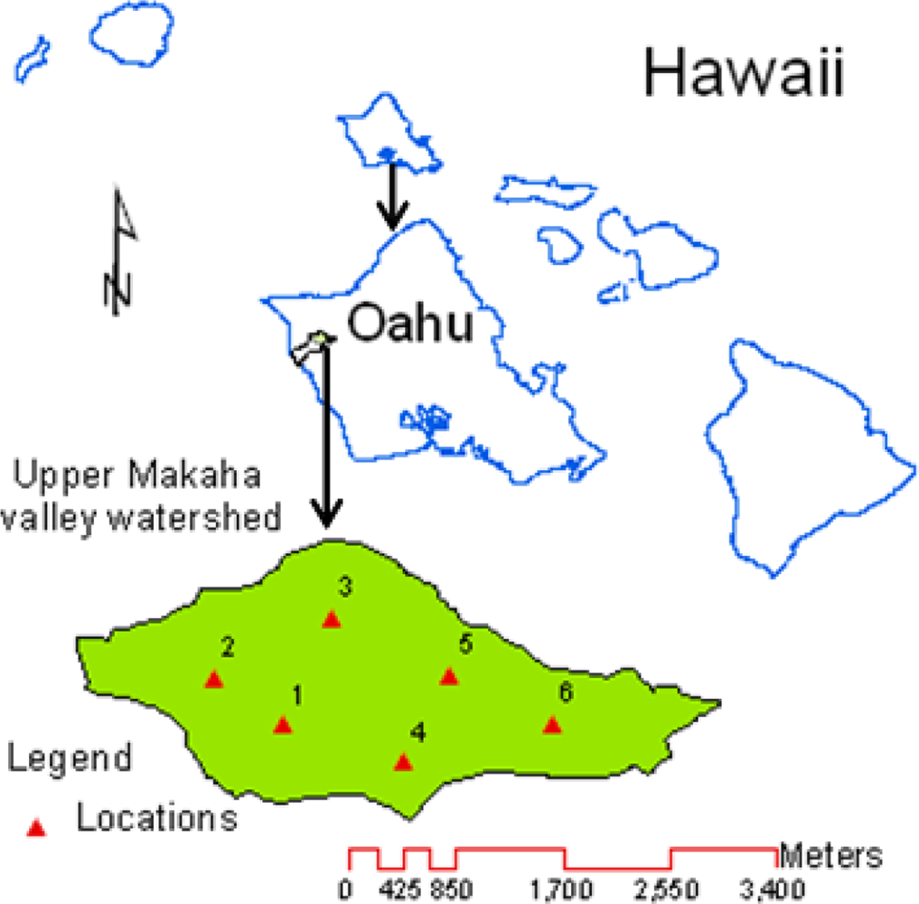
The Mākaha Valley watershed is located in the dry leeward side of the island of O’ahu, HI, USA (Figure 1). This watershed has been the home of a long-term hydrologic study aiming at determining the effects of rainfall variability, groundwater pumping, and invasive species on its hydrology and water quality [17]. The watershed has been instrumented with EC-20, ML2x, and SM200 sensors, and other equipment for real-time monitoring of water budget components. The objectives of this study were to (i) study the spatial variability of ρb, θt, CC, EC, and pH of the upper Mākaha Valley watershed soil, (ii) explore the effect of variations in ρb and θt on soil water content dynamics, and (iii) establish field calibration equations for EC-20, ML2x, and SM200 sensors to improve their performance.
2. Materials and Methods
2.1. Soil Water Content Sensing Devices
The sensors calibrated during this study were the EC-20, ML2x, and SM200 (Table 1). The calibration equation of the EC-20 is a linear function that relates EC-20 readings (V) to the actual soil water content. There is a linear correlation between soil water content measured with the ML2x and the square root of the dielectric constant (√ɛ) [18,19]. The SM200 probe has a similar calibration equation as that of the ML2x.
2.2. Experimental Locations
Field calibrations of the selected sensors were performed at two depths of six monitoring locations across the upper Mākaha Valley sub-watershed (Figure 1). These locations, referred to as locations 1 through 6 from here onward, were initially selected to represent the spatial variations of the topography, soil, and vegetation covers across the study area (Table 2). Soils in the lower valley are less permeable than those along the valley ridges. The soils over the valley floor and along the southeastern ridge of the upper valley are mainly clay loam, silty loam, and silty clay [20].
2.3. Soil Properties
Disturbed and undisturbed soil core samples were collected in three replicates from each depth of the six locations. The undisturbed soil core samples (radius = 2.5 cm; height = 7.5 cm) were collected with a sludge hammer soil sampler (Soilmoisture Equipment Crop. Santa Barbara, CA, USA). The trimmed soil cores were sealed with plastic caps, placed in labeled zip-lock plastic bags, and taken to the laboratory to measure their ρb and θt following the standard procedures described by Grossman and Reinsch [21] and Flint and Flint [22], respectively.
Replicates of the disturbed bulk soil samples were thoroughly mixed to produce a representative sample for each depth and location. These samples were air dried and sieved (<2 mm); a sub-sample was used to determine particle size distribution using the hydrometer method [23]. The textural triangle of the United States Department of Agriculture (USDA) classification scheme was used to determine the soil particle size distributions. Color schemes were used to determine the NRCS (Natural Resources Conservation Services) soil series information. EC and pH of these samples were measured from their 1:2 soil:water solutions with a multi-functional sympHony® meter (Model SB90M5; Batavia, IL, USA) and the respective electrodes.
2.4. Calibration Procedure
Two units of each EC-20, ML2x, and SM200 sensor were installed at 20 and 80 cm depths at locations 1 through 6 following standard procedures [8]. Various soil water content levels ranging between field capacity (∼0.23 cm3 cm−3) and saturation (∼0.59 cm3 cm−3) were generated by intermittently applying water at and surrounding the sensor installation points. Watermark soil matric potential sensors were used to monitor the soil water potential at various soil water content levels. The soil water sensors and matric potential sensors were logged with their corresponding data loggers at 1-min intervals. At least 3 uniform sensor readings were averaged and used with the corresponding actual water content determined in the laboratory from intact soil core samples collected in three replicates from the close proximity of the sensors’ zone of influence such that the center of the soil cores aligned with the center of the individual sensor. These samples were used to determine actual soil water content following the thermo-gravimetric method. These samples were also used to determine ρb and θt. Total porosity was also estimated from the following equation:
2.5. Calibration Equations and Data Analyses
Values of actual soil water content were plotted versus the respective readings (V) of the EC-20, ML2x, and SM200 to establish field calibration equations separately for the two depths (20 and 80 cm) at each location. A factorial analysis of variance (ANOVA) was conducted to evaluate the effect of soil depths and locations on ρb, θt, CC, EC, and pH using Statistix software package [24]. The coefficient of correlation (r), which represents the degree of association between the calculated and the actual water content; the root mean square error (RMSE), which represents the accuracy of calibration equation to predict actual water content; and the mean bias error (MBE), which is an indicator of sensor’s accuracy in form of the difference between means of the calculated and actual water contents, were used to evaluate the field and default calibration equations. The RMSE (cm3 cm−3) and MBE (cm3 cm−3) were calculated as follows:
3. Results and Discussion
3.1. Selected Soil Properties
Across the six soil water content monitoring locations, the soils at 20 cm depth had larger CC than those at 80 cm depth (Table 3). Clay content at 20 cm depth ranged from 157 at location 6 to 610 g kg−1 at location 2; whereas, at 80 cm depth, the CC values ranged from 288 at locations 4 and 5 to 690 g kg−1 at location 2. Soil from both depths at locations 1 and 4 were clay loam. Locations 2 and 3 had clay soils at both depths; whereas, at location 5, loam and sandy loam soils existed at 20 and 80 cm soil depths, respectively. Soil from the 80 cm depth at location 6 was silty clay. Soils at location 6 had the smallest CC among the other sampling locations. Different NRCS soil series were found across the watershed. Location 1 had Molisol, location 2 had Inceptisol, and locations 3 through 5 had Ultisol. Andisols, formed by weathering of volcanic ash under well-drained conditions, dominated location 6; they are characterized by low bulk density (Table 3) and are favorable for keeping aerobic conditions [25].
Larger ρb was observed at 80 cm depth than at 20 cm depth across the six locations except at location 4 (Table 3). The opposite was expected for θt, given the inverse relationship between θt and ρb. Smaller ρb had resulted in larger θt given their inverse relationship (Equation (1)). At the 20 cm depth, ρb ranged from 0.49 at locations 6 to 0.95 g cm−3 at location 4; however, at 80 cm depth, it ranged from 0.72 at location 6 to 1.27 g cm−3 at location 1. At the 20 cm depth, θt ranged from 0.66 at location 4 to 0.72 cm3 cm−3 at location 5; whereas, at 80 cm depth, it varied between 0.56 at location 1 and 0.67 cm3 cm−3 at locations 4.
The values of EC at 20 cm soil depth were almost double of those at 80 cm soil depth at locations 1 through 3; whereas, at locations 4 and 5, the EC values at 20 cm soil depth were 1.5 and 1.2 times those at 80 cm soil depth, respectively (Table 3). At 20 cm soil depth, the EC ranged from 426 at location 3 to 2,016 μS cm−1 at location 1; whereas, at 80 cm soil depth, it ranged from 222 at location 3 to 1,270 μS cm−1 at location 4. Decomposition of the organic matter from the tree litter might have resulted in the larger EC values of the soil samples of the 20 cm soil layer. Reduction in pH of the top soil layers at locations 1 through 3 might have also resulted from the decomposition of organic matter. The soils from the two depths of the six locations were acidic to neutral as their pH varied from 4.24 at 20 cm depth at location 2 to 5.81 at 20 cm depth at location 5.
ANOVA results showed a significant (P < 0.05) increase in ρb and EC values and a significant (P < 0.05) decrease in θt with increase in soil depth (Table 4). This may be due to compaction as a result of the overburden from the above soil load. Soil compaction enhanced ρb and thus reduced θt as shown by Equation (1). There was no significant effect of soil depth on CC and soil pH. Location had a significant (P < 0.05) effect on ρb, θt, and EC and a highly significant (P < 0.01) effect on CC.
3.2. Spatial Variability of Bulk Density and Total Porosity
In general, major soil properties including ρb and θt are consistent for a given soil type, series or order. Variations in ρb and θt are due to many factors such as high organic matter, CC or both. Most of the shrink-swell clays exhibited variability in ρb and θt. The shrink-swell behavior of the soils at locations 1 through 5 was confirmed from the good agreement between the actual θt and those calculated from Equation 1 (Figure 2). Small CC at location 6 suppressed soil shrinking and swelling at this location resulting in a weak correlation (r < 0.4) between the actual and calculated θt.
Pearson’s correlation test was conducted to correlate ρb and θt at 20 and 80 cm depths. Overall, there was a non-significant inverse relationship between ρb and θt except at 20 cm depth where a stronger (r = −0.93) inverse significant (P < 0.05) relationship existed. The strongest (r = 0.95) significant (P < 0.05) relationship between ρb at 20 and 80 cm depths reflected the increasing trend of ρb with soil depth at all experimental locations.
3.3. Soil Water Content Dynamics due to Spatial Variability of Bulk Density and Total Porosity
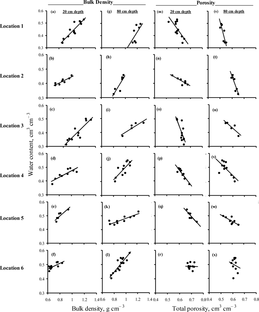
There was a linear increase in ρb and a linear decrease in θt with increase in soil water content at all depths and locations (Figure 3). Slopes of the ρb—water content and θt—water content models for the two depths and six locations were non-uniform reflecting a great spatial variability in these properties. This was an indicator of great soil water content dynamics due to shrinking and swelling—induced changes in ρb and θt. Such behavior of water content dynamics emphasized the need for site-specific calibration equations for soil water content sensors. There were weak θt—water content relationships (r = 7E-04, 0.02) at location 6 [Figures 3(r,x)] partially due to high ash and organic matter contents and partially due to poor structure of highly weathered soil (personal observations). Volcanic ash soils are classified as an Andisol with low densities and assumption of ρs = 2.65 g cm−3 may not be valid for these soils [25]. Moreover, Andisol usually have peculiar permittivity relations due to high surface area and low densities [26–30]. Our results showed that variations in ρb can affect soil water content estimation of high CC soils due to their shrink-swell behavior. Fares et al. [31] and Polyakov et al. [32] reported similar results for a sandy clay loam soil and for a weathered clay loam soil, respectively. Yule [33] and Smith [34] have reported errors in volumetric water content calculation made from ρb information when the ρb was not determined at the right moisture content.
3.4. Field Calibration of Sensors
Since soil depths and locations had significant effect on ρb, θt, CC, and EC (Table 4) in addition to the significant effect of ρb and θt on soil water content dynamics (Figure 3), field calibration equations for each sensor were established for each depth and location (Table 5). These site-specific field calibration equations of the EC-20, ML2x, and SM200 accurately predicted the actual water content (r > 0.88; RMSE 0.011 to 0.054 cm3 cm−3), compared with their respective default equations (r > 0.86; RMSE 0.026 to 0.247 cm3 cm−3). The values of RMSE and MBE of the actual water content and the calculated water content using default equations are inside the parentheses in Table 5. The values of MBE for the site-specific field calibration equations were smaller than those of their corresponding default equations indicating that the site-specific field calibration equations had significantly improved the accuracy of soil water content measurements of these sensors. On the other hand, the default calibration equations substantially under-estimated (larger absolute negative value of MBE) the actual water content compared with their corresponding site-specific field calibration equations (smaller MBE).
The watershed-scale field calibration equations (one equation of each sensor for all depths and locations) of the three sensors seem to substantially (P < 0.001) improve the accuracy of the tested sensors (Table 6). Estimation of actual water content using these new equations resulted in smaller RMSE and MBE as compared with their corresponding default equations. The ML2x exhibited the highest improvement in its accuracy with the use of the new calibration equation (r = 0.81; RMSE 0.038 cm3 cm−3) over its default equation (r = 0.79; RMSE 0.189 cm3 cm−3).
Similar improvement in the accuracy of the SM200 was achieved with the watershed-scale field calibration equations (RMSE 0.042 cm3 cm−3) compared with the default equation (RMSE 0.155 cm3 cm−3). There was a better agreement between actual water content and that measured by the SM200 watershed-scale field calibration equation (MBE −0.001 cm3 cm−3) than between actual water content and that determined by the default equation (MBE −0.126 cm3 cm−3). EC-20 showed the least improvement in its accuracy among the tested sensors with the use of watershed-scale field calibration equation (RMSE 0.054 cm3 cm−3; MBE −0.034 cm3 cm−3) compared to that of its default equation (RMSE 0.068 cm3 cm−3; MBE −0.014 cm3 cm−3).
The performance of the default and watershed site-specific calibration equations in tracking the actual water content is detailed in Figure 4. There was a minimal difference between the performance of the field and the default (MBE −0.034 cm3 cm−3 vs. −0.014 cm3 cm−3) equations of EC-20 (Figure 4(a); Table 6).
4. Conclusions
The effect of spatial variability of ρb, θt, CC, and EC on the performance of EC-20, ML2x, and SM200 sensors installed at 20 and 80 cm depths on six locations across the forested upper Mākaha Valley watershed in O’ahu (Hawai’I, USA) was studied. The studied soil properties significantly varied as a function of the water content monitoring depths and locations. Field calibration equations for the three tested sensors improved their performance for accurate measurement of actual soil water content.
The default equations of the ML2x and SM200 showed substantial under-estimations of actual water content; whereas, the field calibration equations of these sensors substantially improved their accuracy of measuring actual water content. The EC-20 default equation performed better than the default equations of the other two sensors. Moreover, there was no significant difference in the performance of the default and the field calibration equations of EC-20. EC-20 had the least improvement in its accuracy with the use of field calibration equation as compared with the other two sensors. Overall, the field calibration equations were more accurate in estimating soil water content (higher P, r and lower RMSE, MBE) than their corresponding default equations. The tested sensors need site-specific calibrations for accurate measurement of actual water content of these highly weathered tropical soils. The field calibration equations can mitigate the effects of varying soil properties and improve the accuracy of the tested sensors.
Acknowledgments
This project was supported by two grants from the US Department of Agriculture: (1) Cooperative State Research, Education and Extension Service grant number 2004-34135-15058, (2) McIntire-Stennis formula grant number 2006-34135-17690. The authors wish to thank the Honolulu Board of Water Supply for cooperation, and Amjad Ahmad, Nghia Dai Tran, Mohammad Safeeq, Alan Mair and other members of the Watershed Hydrology Laboratory for their help during the field work.
References
- Hawley, ME; Jackson, TJ; McCuen, RH. Surface soil moisture variation on small agricultural watersheds. J. Hydrol 1983, 62, 179–200. [Google Scholar]
- Reynolds, SG. The gravimetric method of soil moisture determination. III. An examination of factors influencing soil moisture variability. J. Hydrol 1970, 11, 288–300. [Google Scholar]
- Western, AW; Blöschl, G. On the spatial scaling of soil moisture. J. Hydrol 1999, 217, 203–224. [Google Scholar]
- Gómez-Plaza, A; Martínez-Mena, M; Albaladejo, J; Castillo, VM. Factors regulating spatial distribution of soil water content in small semiarid catchments. J. Hydrol 2001, 253, 211–226. [Google Scholar]
- Hu, W; Shao, MA; Wang, QJ; Reichardt, K. Soil water content temporal-spatial variability of the surface layer of a loess plateau hillside in china. Sci. Agric 2008, 65, 277–289. [Google Scholar]
- Paige, GB; Keefer, TO. Comparison of field performance of multiple soil moisture sensors in a semi-arid rangeland. J. Am. Water Resour. Assoc 2008, 44, 121–135. [Google Scholar]
- Gardner, WH. Water content. In Methods of Soil Analysis, Part 1 Physical and Mineralogical Methods; SSSA Book Ser 5; Klute, A, Ed.; SSSA: Madison, WI, USA, 1986; pp. 493–544. [Google Scholar]
- Fares, A; Polyakov, V. Advances in crop water management using capacitive water sensors. Adv. Agron 2006, 90, 43–77. [Google Scholar]
- Robinson, DA; Campbell, CS; Hopmans, JW; Hornbuckle, BK; Jones, SB; Knight, R; Ogden, F; Selker, J; Wendroth, O. Soil moisture measurement for ecological and hydrological watershed-scale observatories: A review. Vadose Zone J 2008, 7, 358–389. [Google Scholar]
- Decagon Devices, Inc. ECH2O Utility Mobile for Windows Handheld PCs Operator’s Manual, 2002. Available online: http://www.decagon.com/literature/manuals/Ech2oUtilityMobileManual.pdf/ (accessed on 12 March 2009).
- Dynamax Inc. ThetaProbe Type ML2x, 2009, Available online: ftp://ftp.dynamax.com/DynamaxPDF/irrigation-controls/ML2x.pdf (accessed on 12 March 2009).
- Foley, JL; Harris, E. Field calibration of ThetaProbe (ML2x) and ECHO probe (EC-20) soil water sensors in a Black Vertosol. Aust. J. Soil Res 2007, 45, 233–236. [Google Scholar]
- Fares, A; Hamdhani, H; Jenkins, DM. Temperature-dependent scaled frequency: Improved accuracy of multisensor capacitance probes. Soil Sci. Soc. Am. J 2007, 71, 894–900. [Google Scholar]
- Czarnomski, NM; Moore, GW; Pypker, TG; Licata, J; Bond, BJ. Precision and accuracy of three alternative instruments for measuring soil water content in two forest soils of the Pacific Northwest. Can. J. For. Res 2005, 35, 1867–1876. [Google Scholar]
- Logsdon, SD; Hornbuckle, B. Soil moisture probes for dispersive soils. Proceedings of TDR 2006: Third International Symposium and Workshop on Time Domain Reflectometry for Innovative Soils Applications; Purdue University: West Lafayette, IN, USA, 2006. Available online: https://engineering.purdue.edu/TDR/Papers/13_Paper.pdf (accessed on 12 March 2009). [Google Scholar]
- Hu, Y; Vu, H; Hubble, D. Water content measurement in highly plastic clay using dielectric based probes. Can. Geotech. J 2010, 41, 997–1010. [Google Scholar]
- Fares, A. Determining the Impacts of Water Pumping and Alien Species Invasion on Stream Flow for a Sustainable Water Resource Management in Mākaha Valley; Project report submitted to the Board of Water Supply; University of Hawaii: Honolulu, HI, USA; September; 2007. [Google Scholar]
- Whalley, WR. Considerations on the use of time-domain reflectometry (TDR) for measuring soil moisture content. J. Soil Sci 1993, 44, 1–9. [Google Scholar]
- White, IK; Zegelin, JH; Topp, GC. Comments on ‘Considerations on the use of time-domain reflectometry (TDR) for measuring soil water content’ by W.R. Whalley. J. Soil Sci 1994, 45, 503–508. [Google Scholar]
- Foote, DE; Hill, EL; Nakamura, S; Stephens, F. Soil Survey of the Islands of Kauai, Oahu, Maui, Molokai, and Lanai, State of Hawaii; United States Department of Agriculture, United States Printing Office: Washington, DC, USA, 1972. [Google Scholar]
- Grossman, RB; Reinsch, TG. Bulk density and linear extensibility. In Methods of Soil Analysis, Part 4; SSSA Book Ser 5; Dane, JH, Topp, GC, Eds.; SSSA: Madison, WI, USA, 2002; pp. 201–254. [Google Scholar]
- Flint, LE; Flint, AL. Porosity. In Methods of Soil Analysis, Part 4; SSSA Book Ser 5; Dane, JH, Topp, GC, Eds.; SSSA: Madison, WI, USA, 2002; pp. 241–254. [Google Scholar]
- Gee, GW; Or, D. Particle-size analysis. In Methods of Soil Analysis, Part 4; SSSA Book Ser 5; Dane, JH, Topp, GC, Eds.; SSSA: Madison, WI, USA, 2002; pp. 255–293. [Google Scholar]
- Analytical Software. User’s Manual: STATISTIX8; Analytical Software: Tallahassee, FL, USA, 2003. [Google Scholar]
- Chu, HY; Hosen, Y; Yagi, K; Okada, K; Ito, O. Soil microbial biomass and activities in a Japanese. Andisol as affected by controlled release and application depth of urea. Biol. Fertil. Soils 2005, 42, 89–96. [Google Scholar]
- Weitz, AM; Grauel, WT; Keller, M; Veldkamp, E. Calibration of time domain reflectometry technique using undisturbed soil samples from humid tropical soils of volcanic origin. Water Resour. Res 1997, 33, 1241–1249. [Google Scholar]
- Tomer, MD; Clothier, BE; Vogeler, I; Green, S. A dielectric—Water content relationship for sandy volcanic soils in New Zealand. Soil Sci. Soc. Am. J 1999, 63, 777–781. [Google Scholar]
- Veldkamp, E; O’Brien, JJ. Calibration of a frequency domain reflectoetry sensor for humid tropical soils of volcanic origin. Soil Sci. Soc. Am. J 2000, 64, 1549–1553. [Google Scholar]
- Miyamoto, T; Annaka, T; Chikushi, J. Soil aggregate structure effects on dielectric permittivity of an Andisol measured by time domain reflectometry. Vadose Zone J 2003, 2, 90–97. [Google Scholar]
- Regalado, CM; Ritter, A; Rodrguez-Gonzalez, RM. Performance of the commercial WET capacitance sensor as compared with Time Domain Reflectometry in volcanic soils. Vadoze Zone J 2007, 6, 244–254. [Google Scholar]
- Fares, A; Buss, P; Dalton, M; El-Kadi, AI; Parsons, LR. Dual field calibration of capacitance and neutron sensors in a shrinking-swelling clay soil. Vadose Zone J 2004, 3, 1390–1399. [Google Scholar]
- Polyakov, V; Fares, A; Ryder, MH. Calibration of capacitance system for measuring water content of tropical soil. Vadose Zone J 2005, 4, 1004–1010. [Google Scholar]
- Yule, DF. Volumetric calculations in cracking clay soils. In The Properties and Utilization of Cracking Clay Soils; Reviews in Rural Science No 5; McGarity, JW, Hoult, EH, So, HB, Eds.; University of New England: Armidale, NSW, Australia, 1984; pp. 136–140. [Google Scholar]
- Smith, GD. Soil constituent and prehistory effects on aggregates porosity in cracking clays. In The Properties and Utilization of Cracking Clay Soils; Reviews in Rural Science, No 5; McGarity, JW, Hoult, EH, So, HB, Eds.; University of New England: Armidale, NSW, Australia, 1984; pp. 109–115. [Google Scholar]


| Sensors | Operating frequency, MHz | Default Calibration Equation |
|---|---|---|
| EC-20 | 5 | y = 0.695x − 0.29 |
| ML2x | 100 | y = 0.560x3 − 0.762x2 + 0.762x − 0.063 |
| SM200 | 100 | y = 1.611x5 − 5.48x4 + 7.248x3 − 4.61x2 + 1.917x − 0.071 |
y: actual volumetric soil water content (cm3 cm−3); x: sensor readings (V).
| Location | Elevation, m | Ksat, cm h−1 | Depth, cm | NRCS Soil Series | Clay | Sand | USDA Soil texture |
|---|---|---|---|---|---|---|---|
| g kg−1 | |||||||
| 1 | 343 | 90.2 | 20 | Mollisol | 313 | 269 | Clay loam |
| 80 | Mollisol | 313 | 269 | Clay loam | |||
| 2 | 477 | 10.8 | 20 | Inceptisol | 610 | 308 | Clay |
| 80 | Inceptisol | 690 | 250 | Clay | |||
| 3 | 538 | 31.4 | 20 | Ultisol | 521 | 167 | Clay |
| 80 | Ultisol | 640 | 250 | Clay | |||
| 4 | 601 | 63.8 | 20 | Ultisol | 313 | 218 | Clay loam |
| 80 | Ultisol | 288 | 320 | Clay loam | |||
| 5 | 609 | 16.5 | 20 | Ultisol | 263 | 421 | Loam |
| 80 | Ultisol | 288 | 661 | Sandy loam | |||
| 6 | 725 | 19.3 | 20 | Andisol | 157 | 371 | Loam |
| 80 | Andisol | 230 | 218 | Silt loam | |||
| Location | Depth (cm) | ρb g (cm−3) | θt cm3 (cm−3) | EC# μS (cm−1) | pH# |
|---|---|---|---|---|---|
| 1 | 20 | 0.93 | 0.69 | 2016 | 5.01 |
| 80 | 1.27 | 0.56 | 840 | 5.52 | |
| 2 | 20 | 0.86 | 0.67 | 802 | 4.24 |
| 80 | 1.06 | 0.60 | 480 | 4.29 | |
| 3 | 20 | 0.83 | 0.67 | 426 | 4.60 |
| 80 | 0.97 | 0.58 | 222 | 4.69 | |
| 4 | 20 | 0.95 | 0.66 | 1888 | 5.65 |
| 80 | 0.93 | 0.67 | 1270 | 4.91 | |
| 5 | 20 | 0.69 | 0.72 | 1220 | 5.81 |
| 80 | 0.93 | 0.61 | 1024 | 4.89 | |
| 6 | 20 | 0.49 | 0.80 | 1189 | 4.88 |
| 80 | 0.72 | 0.75 | 959 | 5.09 |
#Electrical conductivity and pH measurements were made on 1:2 soil:water solutions.
| Factors | Bulk Density | Total Porosity | Clay Contents | Electrical Conductivity | pH |
|---|---|---|---|---|---|
| Depth | 0.0125* | 0.0153* | NS | 0.0336* | NS |
| Location | 0.0220* | 0.0463* | 0.0026** | 0.0355* | NS |
| Interaction | NS | NS | NS | NS | NS |
*:significant;**:highly significant; NS: not significant.
| Location | Depth | Sensor | a¶ × 10−2 | b§ × 10−2 | r | RMSE ÷ 102, cm3 cm−3 | MBE ÷ 102, cm3 cm−3 | n |
|---|---|---|---|---|---|---|---|---|
| 1 | 20 | EC-20 | 0.04 | −1.71 | 0.954(0.945) | 3.63 (12.0) | 2.82 (10.0) | 16 |
| ML2x | 48.68 | 20.31 | 0.917(0.919) | 3.00 (24.7) | −0.15 (−24.5) | 16 | ||
| SM200 | 30.10 | 29.85 | 0.968(0.974) | 3.73 (14.9) | 0.00 (−13.3) | 16 | ||
| 80 | EC-20 | 0.04 | −0.20 | 0.916(0.917) | 3.87 (7.31) | 2.81 (4.45) | 12 | |
| ML2x | 47.08 | 17.59 | 0.913(0.914) | 2.67 (21.3) | 0.00 (−21.1) | 12 | ||
| SM200 | 24.97 | 28.25 | 0.911(0.903) | 2.70 (11.5) | −0.00 (−8.63) | 12 | ||
| 2 | 20 | EC-20 | 0.03 | 11.51 | 0.917(0.917) | 1.79 (7.19) | −0.33 (−4.65) | 16 |
| ML2x | 31.74 | 24.28 | 0.944(0.937) | 1.45 (20.7) | −0.03 (−20.5) | 16 | ||
| SM200 | 27.05 | 32.38 | 0.930(0.939) | 1.62 (19.9) | −0.00 (−19.0) | 16 | ||
| 80 | EC-20 | 0.05 | −7.17 | 0.929(0.928) | 3.60 (2.61) | 3.19 (−0.39) | 12 | |
| ML2x | 26.0 | 25.01 | 0.929(0.926) | 1.63 (18.1) | −0.00 (−17.7) | 12 | ||
| SM200 | 18.39 | 31.25 | 0.960(0.957) | 1.59 (13.4) | 1.00 (−10.3) | 12 | ||
| 3 | 20 | EC-20 | 0.04 | −2.30 | 0.933(0.933) | 5.40 (6.04) | −4.75 (−2.45) | 16 |
| ML2x | 55.24 | 13.01 | 0.921(0.919) | 2.79 (21.3) | −0.08 (−21.0) | 16 | ||
| SM200 | 27.05 | 32.38 | 0.921(0.922) | 2.80 (12.7) | −0.00 (−12.3) | 16 | ||
| 80 | EC-20 | 0.04 | 0.12 | 0.935(0.935) | 1.66 (5.10) | 1.26 (4.46) | 10 | |
| ML2x | 19.49 | 28.66 | 0.920(0.925) | 1.18 (13.8) | −0.00 (−13.0) | 10 | ||
| SM200 | 42.16 | 24.84 | 0.891(0.891) | 1.36 (9.28) | 0.00 (−0.14) | 10 | ||
| 4 | 20 | EC-20 | 0.04 | 15.1 | 0.909(0.909) | 2.14 (6.13) | 1.18 (−2.16) | 18 |
| ML2x | 24.25 | 32.0 | 0.884(0.877) | 1.99 (23.8) | 0.27 (−23.4) | 18 | ||
| SM200 | 17.64 | 38.07 | 0.878(0.890) | 2.04 (18.4) | −0.00 (−16.5) | 18 | ||
| 80 | EC-20 | 0.04 | −0.12 | 0.917(0.917) | 1.61 (5.78) | −16.0 (−4.08) | 14 | |
| ML2x | 38.53 | 21.79 | 0.883(0.864) | 0.75 (19.6) | −0.00 (−19.4) | 14 | ||
| SM200 | 16.81 | 40.36 | 0.917(0.912) | 3.50 (16.5) | −0.95 (−13.8) | 14 | ||
| 5 | 20 | EC-20 | 0.03 | 15.02 | 0.908(0.908) | 2.21 (6.83) | −0.53 (−2.62) | 12 |
| ML2x | 60.96 | −1.05 | 0.897(0.888) | 3.08 (13.1) | 2.10 (−12.9) | 12 | ||
| SM200 | – | – | – | – | – | – | ||
| 80 | EC-20 | 0.04 | −4.12 | 0.911(0.911) | 10.7 (6.18) | −10.6 (−5.38) | 16 | |
| ML2x | 33.44 | 18.39 | 0.903(0.910) | 1.82 (8.91) | 0.17 (−7.73) | 16 | ||
| SM200 | – | – | – | – | – | – | ||
| 6 | 20 | EC-20 | 0.04 | −0.20 | 0.942(0.942) | 12.3 (6.83) | −12.2 (−5.73) | 18 |
| ML2x | 31.09 | 20.04 | 0.906(0.886) | 0.95 (9.02) | 0.00 (−8.68) | 12 | ||
| SM200 | – | – | – | – | – | – | ||
| 80 | EC-20 | 0.06 | −9.29 | 0.961(0.961) | 5.26 (4.93) | 5.10 (−4.66) | 16 | |
| ML2x | 26.51 | 30.51 | 0.943(0.953) | 1.08 (16.5) | −0.00 (−15.9) | 7 | ||
| SM200 | – | – | – | – | – | – | ||
¶slope;§y intercept.
| Sensor | N | Calibration | a¶ | b§ | P | r | RMSE ÷ 102, cm3 cm−3 | MBE, ÷ 102, cm3 cm−3 |
|---|---|---|---|---|---|---|---|---|
| EC-20 | 176 | Field | 0.3 | 0.0969 | 4.24E-33 | 0.75 | 5.41 | −3.36 |
| Default | 0.695 | −0.29 | 4.24E-33 | 0.75 | 6.84 | −1.37 | ||
| ML2x | 160 | Field | 0.2592 | 0.2768 | 1.41E-38 | 0.81 | 3.79 | 0.002 |
| Default | # | # | 1.34E-35 | 0.79 | 18.9 | −17.7 | ||
| SM200 | 113 | Field | 0.2109 | 0.3334 | 2.06E-22 | 0.75 | 4.22 | −0.103 |
| Default | # | # | 4.46E-23 | 0.76 | 15.5 | −12.6 | ||
¶slope;§y intercept;#:Parameters are given in Table 1.
© 2011 by the authors; licensee MDPI, Basel, Switzerland. This article is an open access article distributed under the terms and conditions of the Creative Commons Attribution license (http://creativecommons.org/licenses/by/3.0/).
Share and Cite
Abbas, F.; Fares, A.; Fares, S. Field Calibrations of Soil Moisture Sensors in a Forested Watershed. Sensors 2011, 11, 6354-6369. https://doi.org/10.3390/s110606354
Abbas F, Fares A, Fares S. Field Calibrations of Soil Moisture Sensors in a Forested Watershed. Sensors. 2011; 11(6):6354-6369. https://doi.org/10.3390/s110606354
Chicago/Turabian StyleAbbas, Farhat, Ali Fares, and Samira Fares. 2011. "Field Calibrations of Soil Moisture Sensors in a Forested Watershed" Sensors 11, no. 6: 6354-6369. https://doi.org/10.3390/s110606354
APA StyleAbbas, F., Fares, A., & Fares, S. (2011). Field Calibrations of Soil Moisture Sensors in a Forested Watershed. Sensors, 11(6), 6354-6369. https://doi.org/10.3390/s110606354