Direction-of-Arrival Estimation Based on Joint Sparsity

Abstract

We present a DOA estimation algorithm, called Joint-Sparse DOA to address the problem of Direction-of-Arrival (DOA) estimation using sensor arrays. Firstly, DOA estimation is cast as the joint-sparse recovery problem. Then, norm is approximated by an arctan function to represent joint sparsity and DOA estimation can be obtained by minimizing the approximate norm. Finally, the minimization problem is solved by a quasi-Newton method to estimate DOA. Simulation results show that our algorithm has some advantages over most existing methods: it needs a small number of snapshots to estimate DOA, while the number of sources need not be known a priori. Besides, it improves the resolution, and it can also handle the coherent sources well.

1. Introduction

Direction-of-Arrival (DOA) estimation using sensor arrays has been an active research area, playing a fundamental role in many applications involving electromagnetic, acoustic, and communication systems [1]. Many classical algorithms are available, and the popular methods include beamforming [2], MUSIC [3], ESPRIT [4] and the maximum likelihood method [5], etc. The beamforming method has low angle resolution and suffers from the Rayleigh resolution limit. MUSIC, ESPRIT and the maximum likelihood method all rely on the statistical properties of the data, and thus, require a sufficiently large number of samples for accurate estimation. Besides, MUSIC and ESPRIT cannot handle strongly coherent sources, while the maximum likelihood method has high computation costs.

The problem of sparse recovery has evolved rapidly recently [6,7] and it has been applied in DOA estimation with array processing. Gorodnitsky et al. [8] used a weighted least-squares algorithm named FOCUSS for DOA estimation, but this algorithm can only be used for single snapshots. Cotter [9] combined multiple measurement vectors (MMV) and matching pursuit (MP) to solve the joint-sparse recovery problem in DOA estimation, but it has low angle resolution. JLZA-DOA is proposed in [10]; it minimizes a mixed L_2,0 norm to deal with the joint-sparse recovery problem, and a fixed point method is used for DOA estimation. This algorithm doesn’t satisfy numerical stability, as matrix inversion is inevitable in every iteration. Stoica et al. [11] presented a novel SParse Iterative Covariance-based Estimation approach, abbreviated SPICE. However, this algorithm needs more snapshots to estimate DOA. Wide-band covariance matrix sparse representation (W-CMSR) is proposed in [12] for DOA estimation of wideband signals. So far, the most successful joint-sparse recovery algorithm for DOA estimation is L1-SVD [13,14]. It combines the SVD step of the subspace algorithms with a sparse recovery method based on l_2,1 –norm minimization. However, the number of sources needs be known a priori.

In this paper, we present Joint-Sparse DOA estimation, abbreviated as JSDOA, for sensor array DOA estimation. First, DOA estimation is cast as a joint-sparse recovery problem. Then, L_2,0 norm is approximated by the arctan function to represent spatial sparsity and DOA estimation can be obtained by minimizing the approximate L_2,0 norm. Finally, the minimization problem is solved by a quasi-Newton method to estimate DOA. The proposed algorithm has some advantages over most existing methods: it needs a small number of snapshots to estimate DOA, an the number of sources need not be known a priori. Besides, it improves the probability of resolution, and it can also handle coherent sources well.

The outline of the paper is as follow. In Section 2, the DOA estimation problem is formulated. The new algorithm, called JSDOA, is proposed in Section 3. In section 4, the validity of the proposed algorithm is proved by a number of simulations. Finally, conclusions are presented in Section 5.

2. Problem Formulation

2.1. DOA Estimation Problem

Consider a linear array consisting of M identical sensors and receiving signals from K narrowband signals s₁(t), s₂(t), ⋯, s_K(t), which arrive at the array from directions θ̄₁, θ̄₂, ⋯ θ̄_K with respect to the line of array. The received signal y_m(t) at the m^th sensor can be written as:

$$y_m(t)=\sum _{k=1}^{K}a({\overline{\theta }}_k)s_k(t)+n_m(t)$$

(1)

where ${\left\{a({\overline{\theta }}_k)\right\}}_{k=1}^K$ denote steering vectors, n_m(t) (m = 1, 2 ⋯, M) stand for the additive noise.

Let y(t) = [y₁(t), y₂(t), ⋯, y_M(t)]^T, n(t) = [n₁(t), ⋯, n_M(t)], Equation (1) can be written as:

$$y(t)=A(\overline{\theta })s(t)+n(t)$$

(2)

where the manifold matrix A (θ̄) consists of the steering vectors ${\left\{a({\overline{\theta }}_k)\right\}}_{k=1}^K$:

$$A(\theta )=\left[a({\overline{\theta }}_1),a({\overline{\theta }}_2),\cdots ,a({\overline{\theta }}_K)\right]$$

Therefore, DOA estimation is to find K and θ̄_k from T snapshots ${\left\{y(t)\right\}}_{t=t_1}^{t_T}$.

2.2. Joint-Sparse Recovery for DOA Estimation Problem

Because sources are sparse in space, DOA estimation with sensor arrays can be expressed as a joint-sparse recovery problem. Let Ω denote the set of possible locations, ${\left\{{\theta }_n\right\}}_{n=1}^N$ denotes a grid that covers Ω. We assume that the grid is fine enough such that the true location parameters of the existing sources lie on the grid. Let:

$$x(t)={[x_1(t), x_2(t), \cdots ,x_N(t)]}^T$$

Then the received signal y_m(t) at the m^th sensor can be written as:

$$y_m(t)=\sum _{n=1}^{N}a({\theta }_n)x_n(t)+n(t)$$

(3)

where the n^th element x_n(t) of x(t) is nonzero only if θ_n = θ̄_k, k ∈ [1,2, ⋯, K] and in that case x_n(t) = s_k(t):

Let Φ = [a(θ₁), a(θ₂), ⋯, a(θ_N)], (3) can be expressed as:

$$y(t)=\Phi x(t)+n(t)$$

(4)

when the number of snapshots is denoted as T, Equation (4) can be written as:

$$Y=\Phi X+N$$

(5)

where Y = [y(t₁), y(t₂), ⋯, y(t_T)], X = [x(t₁), x(t₂), ⋯, x(t_T)]. As we know, X is row-sparse and only K rows have nonzero elements, so DOA estimation can be obtained by a joint-sparse recovery problem, which is also called a multiple measurement vectors (MMV) problem. Using l_p,q norm to express joint sparsity, the MMV problem can be converted to l_p,q norm minimization:

$$\{\begin{array}{ll}\text{min}\hfill & {\Vert X\Vert }_{p,q}\hfill \\ s.t.\hfill & Y=\Phi X+N\hfill \end{array}$$

(6)

where p and q are non-negative, and ‖X‖_p,q is defined as:

$${\Vert X\Vert }_{p,q}=\sum _{i=1}^M{\left({\Vert X(i,:)\Vert }_p\right)}^q$$

(7)

Concretely, Eldar and Mishali [15] use p = 2, q = 1. Chen and Huo [16] study for p = 1, q = 1. The above algorithms do not perform very well for ‖X‖ _2,1 and ‖X‖ _1,1 can’t sufficiently reflect joint sparsity. Considering ‖X‖ _2,0 can reflect joint sparity sufficiently, we minimize ‖X‖ _2,0 norm to solve the MMV problem. However, ‖X‖ _2,0 norm minimization can hardly be solved directly. Therefore, in this paper we approximate ‖X‖ _2,0 norm by an arctan function and estimate DOA by solving an approximate ‖X‖ _2,0 norm minimization problem.

3. Joint-Sparse DOA Estimation Algorithm

In this section, the DOA estimation problem is converted into an approximate ‖X‖ _2,0 norm minimization problem. Firstly, the L_2,0 norm is approximated by an arctan function to construct an approximate ‖X‖ _2,0 norm minimization problem. Then this problem is solved by a quasi-Newton method to estimate DOA.

3.1. Basic Idea of the Proposed Method

Let ξ_i = ‖X(i,:)‖₂, i = 1, 2, ⋯, M, we have:

$${\Vert X\Vert }_{2,0}=\sum _{i=1}^M{\left({\Vert X(i,:)\Vert }_2\right)}^0={\Vert \xi \Vert }_0$$

(8)

where ξ = (ξ₁, ⋯, ξ_M). Considering the following arctan function:

$$f_{\delta }(s)=\frac{2}{\pi }\mathit{arc}\hspace{0.17em}\text{tan}(\frac{s^2}{2{\delta }^2})$$

(9)

where δ is a positive parameter and s is a variable parameter. Then f_δ(s) has the following property:

$$\underset{\delta \to 0}{\text{lim}}{f}_{\delta }(s)=\{\begin{array}{cc}1& s\ne 0\\ 0& s=0\end{array}$$

(10)

Let

$$F_{\delta }(\xi )=\sum _{i=1}^N{f}_{\delta }({\xi }_i)$$

From Equation (10), we have:

$$\underset{\delta \to 0}{\text{lim}}{F}_{\delta }(\xi )={\Vert \xi \Vert }_0$$

(11)

From Equations (8) and (10), then:

$$\underset{\delta \to 0}{\text{lim}}{F}_{\delta }(X)={\Vert X\Vert }_{2,0}$$

So DOA can be obtained by solving the approximate ‖X‖_2,0 norm minimization:

$$\{\begin{array}{ll}\text{min}\hfill & F_{\delta }(X)\hfill \\ s.t.\hfill & Y=\Phi X+N\hfill \end{array}$$

(12)

where δ is a small positive constant. Because noise is unknown, we synchronously hope to minimize F_δ(X) and ${\Vert \Phi X-Y\Vert }_F^2$. Then Equation (12) is converted into a multiple objective optimization:

$$\{\begin{array}{ll}\underset{X}{\text{min}}\hfill & F_{\delta }(X)\hfill \\ \underset{X}{\text{min}}\hfill & {\Vert \Phi X-Y\Vert }_F^2\hfill \end{array}$$

(13)

Using the linear weighting method, Equation (13) can be written as:

$$\underset{x}{\text{min}} L_{\delta ,\lambda }(X)=F_{\delta }(X)+\lambda {\Vert \Phi X-Y\Vert }_F^2$$

(14)

where ‖•‖_F denotes the Frobenious norm and the parameter λ will be discussed in Section 3.2. When the parameter δ is very small, the objective function F_δ(X) is highly unsmoothed and contains a lot of local minimization, so its global minimization is not easy. On the other hand, if the parameter δ is larger, the objective function F_δ(X) is smoother and contains less local minimization. In order to obtain global minimization, we select a decreasing sequence for δ, denoted as:

$$\delta =[{\delta }_1,{\delta }_2,\cdots ,{\delta }_J], {\delta }_{j+1}<{\delta }_j$$

where δ₁ is a relatively large value, and δ_J is a small value. For δ = δ_J−1, the solution of Equation (14) is denoted as x_δj–1, and x_δj–1 is used as the initial value for δ = δ_j, thus we hope the proposed algorithm can escape from getting trapped into a local minimum and reach the global minimization for a small value δ = δ_J.

For some fixed value δ = δ_j, minimization problem Equation (14) is solved by the quasi-Newton method in this paper. One of the most successful quasi-Newton methods is the BFGS algorithm, which is second order convergent and has good numerical stability. Therefore, we use the BFGS algorithm to solve Equation (14) for some fixed value δ = δ_j.

The conjugate gradient for a matrix variable is defined as:

$$\frac{\partial L_{\delta ,\lambda }(X)}{\partial X^{*}}=\frac{1}{2}\left(\frac{\partial L_{\delta ,\lambda }(X)}{\partial X_R}+i\frac{\partial L_{\delta ,\lambda }(X)}{\partial X_I}\right)$$

where X_R and X_l denote the real part and the imaginary part respectively, X^*denotes the conjugate of X. Then the conjugate gradient of L_δ,λ(X) (for its derivation see Appendix I) can be expressed as:

$$\frac{\partial L_{\delta ,\lambda }(X)}{\partial X^{*}}=\frac{1}{2{\delta }^2}\Lambda X-\lambda {\Phi }^{*}(Y-\Phi X)$$

(15)

where

$$\Lambda =\mathit{diag}\left\{{\delta }^2/\left({\xi }_1^4+4{\delta }^4\right), {\delta }^2/\left({\xi }_2^4+4{\delta }^4\right),\cdots ,{\delta }^2/\left({\xi }_n^4+4{\delta }^4\right)\right\}$$

Solving by the BFGS algorithm, the main iterative steps are as follows:

• Search step length t_k, satisfy: $t_k=\underset{t}{\text{min}} L_{{\delta }_j,\lambda } \left(x-t{H}^k\nabla L_{{\delta }_j,\lambda }(X)\right)$

• Iteration: $X^{k+1}=X^k-t_k H^k\frac{\partial L_{\delta ,\lambda }(X^k)}{\partial X^{*}}$

• BFGS adjustment:

  $$H^{k+1}=H^k+\left(1+\frac{{(g^k)}^T{H}^k{g}^k}{{(g^k)}^T{s}^k}\right)\frac{s^k{(s^k)}^T}{{(g^k)}^T{s}^k}-\frac{s^k{(g^k)}^T{H}^k-H^k{g}^k{(s^k)}^T}{{(g^k)}^T{s}^k}$$

  (16)

where s^k = X^k+1 – X^k, $g^k=\frac{\partial L_{\delta ,\lambda }(X^{k+1})}{\partial X^{*}}-\frac{\delta L_{\delta ,\lambda }(X^k)}{\partial X^{*}}$

3.2. Algorithm Description

Based on the above idea, JSDOA can be described as shown in

Table 1. The main steps of JSDOA.

Algorithm 1: joint-sparse DOA estimation
Input: A, y
Initialization:
(1) Set X0 = AT(AAT)−1Y
(2) Select a decreasing sequence δ = [δ1 δ2 ⋯ δJ], set ɛ and parameter λ
Iteration:
(1) for j = 1,2, … J
(2) solving (14) by BFGS algorithm
(2–1) x = xj − 1, H = I (I is unit matrix);
(2–2) while norm (∂Lδj,λ (X)/∂X) > δjɛ;
(2–3) Search step length $\tilde{t}:\tilde{t}=\underset{t}{\text{min}}{L}_{{\delta }_j,\lambda }\left(X-tH\partial L_{{\delta }_j,\lambda }(X)/\partial X\right)$
(2–4) Let X = X – t̃H∂Lδj,λ (X)/∂X
(2–5) Update the matrix by (16)
(2–6) end
(3) Let Xj = X
(4) end
Output: X̂ = XJ, spatial spectrum P(θ̄i) = 10 log10 (‖X̂(i,:)‖2)

.

Remark:

(1) Select parameter λ: in this paper, we select the parameter λ by the α– method [17]. Set f₁(X) = F_δ(X), $f_2(X)={\Vert \mathit{AX}-y\Vert }_F^2$, and minimizing f₁(X) and f₂(X), we have;

$$f_i(X^{(i)})=\underset{x}{\text{min}} f_i(X)\hspace{1em}i=1,2$$

It is easy to know that X⁽ⁱ⁾(i = 1,2) is 0 and A^T(AA^T)⁻¹Y respectively. Then we have:

$$f_{\mathit{ij}}=f_i(X^{(j)})\hspace{1em}i,j=1,2$$

Set λ = λ₂/λ₁ and introduce auxiliary parameter α, we can have:

$$\{\begin{array}{l}\sum _{i=1}^2{f}_{\mathit{ij}}{\lambda }_i=\alpha \hfill \\ \sum _{i=1}^2{\lambda }_i=1\hfill \end{array}$$

Setting the coefficient matrix f(i,j) = f_ij, from the above equations, the solution is:

$$\{\begin{array}{l}[{\lambda }_1,{\lambda }_2]=\frac{e^T{f}^{-1}}{e^T{f}^{-1}e}\hfill \\ \alpha =\frac{1}{e^T{f}^{-1}e}\hfill \end{array}$$

(17)

where e = [1,1]^T, and λ = λ₂/λ₁.

(2) Select parameter δ: In this paper, we set δ_j = γδ_j–1, j = 2, ⋯, J, γ ∈ (0.5,1). Let $\tilde{x}={\text{max}}_i|x_i^0|$, we hope parameter δ₁ satisfies:

$$f_{\delta }(\tilde{x})=\frac{2}{\pi }\mathit{arc}\hspace{0.17em}\text{tan}\hspace{0.17em}(\frac{{\tilde{x}}^2}{2{\delta }_1^2})\le \frac{1}{2}\Rightarrow {\delta }_1\ge \frac{\tilde{x}}{\sqrt{2}}$$

In order to save computation cost, we set ${\delta }_1={\text{max}}_i|x_i^0|/\sqrt{2}$. When δ_J → 0, F_δJ(x) → ‖x‖₀. However, if δ_J is too small, F_δJ(x) will be sensitive to noise, so δ_J shouldn’t be too small.

(3) For coherent sources: Many of popular methods, such as MUSIC and ESPRIT require the assumption that sources are uncorrelated, because the source covariance matrix remains nonsingular so long as none of these sources are coherent. However, the algorithm proposed in this paper doesn’t need to compute the source covariance matrix, and joint sparsity is used to estimate DOA, so the proposed algorithm can handle highly coherent sources as well.

(4) Limitation: The algorithm proposed in this paper suffers from two problems. First, there exist no clear-cut guidelines for the selection of δ_J, especially when knowledge of noise is unknown. Second, the proposed algorithm can’t perform well when the SNR is relatively low.

4. Simulation Results

In this section, we present several numerical simulation results to illustrate the performance of the proposed algorithm. First, we compare the spatial spectrum of JSDOA to those of beamforming [2], MUSIC [3], and L1-SVD [13] under various snapshot scenartios. Next, we compare the spatial spectrum with more than two sources. Then, the probability of resolution is compared. Finally, we compare the spatial spectrum for coherent sources. In the following numerical simulations, we consider a uniform linear array consisting of M = 8 identical sensors and receiving signals are narrowband signals. The sensors are uniformly placed with a spacing of half a wavelength. The interval for the DOA is Ω = [−90,90], we use a uniform grid ${\{{\theta }_n\}}_{n=1}^N$ to cover Ω with a step of 1°, which means N = 181.

4.1. Spatial Spectrum Comparison under Various Snapshots

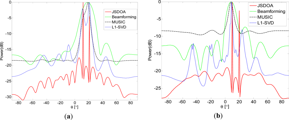
In this simulation, we compare spatial spectrum of different algorithms under various snapshots. We consider two uncorrelated sources located at 13° and 20° with SNR = 10. For JSDOA, we set ${\delta }_1={\text{max}}_i|x_i^0|/\sqrt{2}$, δ_j = γδ_j–1, γ = 0.5, J = 7. In Figures 1(a,b), we set T = 10 and T = 5, respectively. It can be seen from Figure 1 that JSDOA and L1-SVD can resolve the two sources as T = 10. However, only JSDOA can resolve the two sources as T = 5.

4.2. Spatial Spectrum Comparison with More Than Two Sources

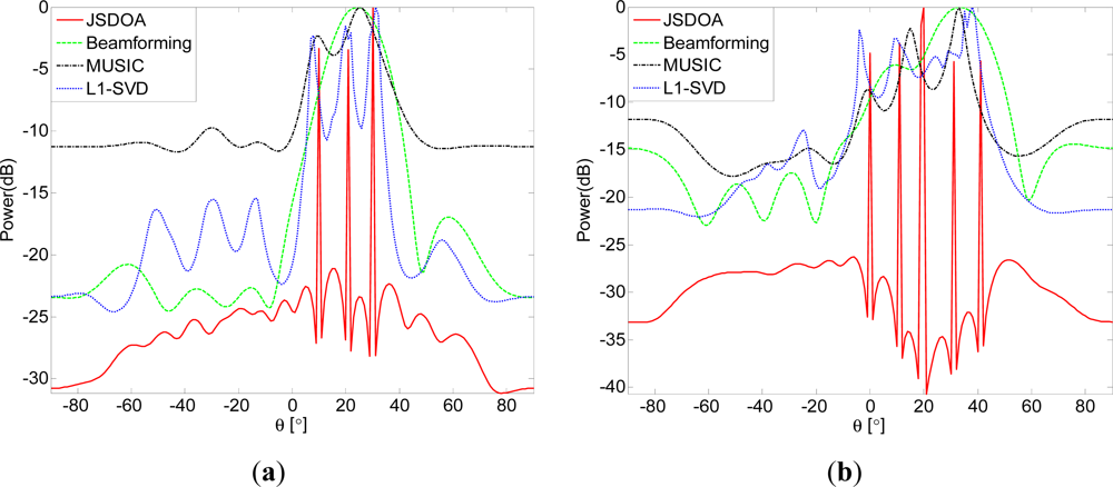
In this simulation, we compare the spatial spectrum of different algorithms with more than two uncorrelated sources. Set SNR = 10, T = 20, ${\delta }_1={\text{max}}_i|x_i^0|/\sqrt{2}$, δ_j = γδ_j–1, γ = 0.5, J = 7. In Figure 2(a), there are three sources located at 10, 20 and 30. In Figure 2(b), there are five sources located at 0, 10, 20, 30 and 40. It is shown from Figure 1 that JSDOA and L1-SVD can resolve the three sources, but only JSDOA can resolve the five sources.

4.3. Probability of Resolution Comparison under Various Conditions

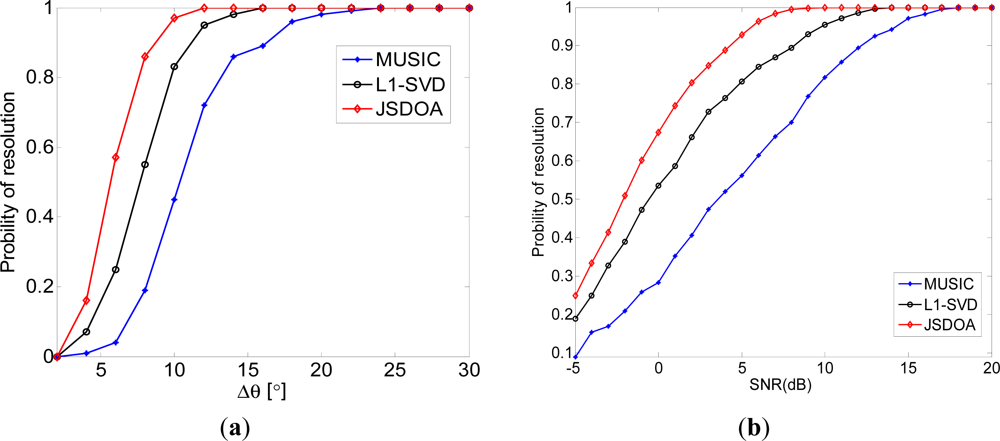
In this simulation, we compare probability of resolution for two uncorrelated sources. JSDOA, MUSIC and L1-SVD are used for comparison and we set T = 5, δ_j = γδ_j–1, γ = 0.5, J = 7. For each Δθ or SNR, 200 independent simulation are carried out. In Figure 3(a), one source is fixed at 10°, the other source is located at 10° + Δθ. vary from 0 to 30. In Figure 3(b), two sources are located at 10° and 20°. SNR vary from −5 to 20. It is shown from Figure 3 that JSDOA has the higher probability of resolution than MUSIC and L1-SVD.

4.4. Spatial Spectrum Comparison for Coherent Sources

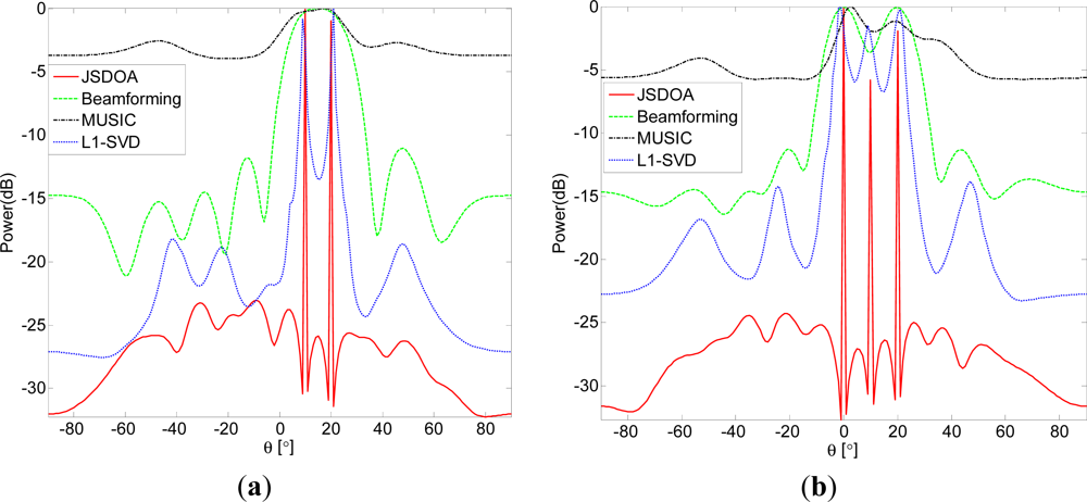
In this simulation, we compare spatial spectrum for completely coherent sources. Set SNR = 10, T = 20, ${\delta }_1={\text{max}}_i|x_i^0|/\sqrt{2}$, δ_j = γδ_j–1, γ = 0.5, J = 7. In Figure 4(a) two coherent sources, located at 10° and 20°, are considered.

In Figure 4(b) three coherent sources, located at 10° and 20°, are considered. It is shown from Figure 4 that JSDOA and L1-SVD can be used to estimate DOA for coherent sources and that JSDOA has higher resolution than L1-SVD.

5. Conclusions

In this paper, a joint-sparse recovery algorithm, called JSDOA, is proposed to estimate DOA with sensor arrays. We pose the DOA estimation problem as a joint-sparse recovery problem, which can be solved by minimizing the approximate L_2,0 norm. In particular, the L_2,0 norm is approximated by an arctan function to represent spatial sparsity and the approximate L_2,0 norm minimization problem is solved by a quasi-Newton method. Finally, the proposed algorithm is examined by simulations. Several advantages over existing DOA estimation algorithms were identified. It can perform well with a limited number of snapshots, while the number of sources need not be known a priori. Besides, it improves the resolution, and it can also handle the coherent sources well.

References

- Krim, H; Viberg, M. Two decades of array signal processing research: The parametric approach. IEEE Signal Process. Mag 1996, 13, 67–94. [Google Scholar]
- Johnson, DH; Dudgeon, DE. Array Signal Processing—Concepts and Techniques; Prentice-Hall: Englewood Cliffs, NJ, USA, 1993. [Google Scholar]
- Schmidt, R. Multiple emitter location and signal parameter estimation. IEEE Trans. Antennas Propag 1986, 34, 276–280. [Google Scholar]
- Roy, R; Kailath, T. Esprit-estimation of signal parameters via rotational invariance techniques. IEEE Trans. Acoust. Speech Signal Process 1989, 37, 984–995. [Google Scholar]
- Stoica, P; Sharman, KC. Maximum likelihood methods for direction-of-arrival estimation. IEEE Trans. Acoust. Speech Signal Process 1990, 38, 1132–1143. [Google Scholar]
- Hyder, M; Mahata, K. An improved smoothed l0 approximation algorithm for sparse representation. IEEE Trans. Signal Process 2010, 58, 2194–2205. [Google Scholar]
- Mourad, N; Reilly, JP. Minimizing Nonconvex Functions for Sparse Vector Reconstruction. IEEE Trans. Signal Process 2010, 58, 3485–3496. [Google Scholar]
- Gorodnitsky, IF; Rao, BD. Sparse signal reconstructions from limited data using FOCUSS: A re-weighted minimum norm algorithm. IEEE Trans. Signal Process 1997, 45, 600–616. [Google Scholar]
- Cotter, S. Multiple Snapshot Matching Pursuit for Direction of Arrival (DOA) Estimation. Proceedings of the European Signal Processing Conference, Poznan, Poland, 3–7 September 2007; pp. 247–251.
- Hyder, MM; Mahata, K. Direction-of-Arrival estimation using a mixed L2.0 morm approximation. IEEE Trans. Signal Process 2010, 58, 4646–4655. [Google Scholar]
- Stoica, P; Babu, P; Li, J. SPICE: A sparse covariance-based estimation method for array processing. IEEE Trans. Signal Process 2011, 59, 629–638. [Google Scholar]
- Liu, ZM; Huang, ZT; Zhou, YY. Direction-of-Arrival estimation of wideband signals via covariance matrix sparse representation. IEEE Trans. Signal Process 2011, 59, 4256–4270. [Google Scholar]
- Malioutov, D; Cetin, M; Willsky, A. A sparse signal reconstruction perspective for source localization with sensor arrays. IEEE Trans. Signal Process 2005, 53, 3010–3022. [Google Scholar]
- Sun, K; lin, Y; Meng, H. Sparse representation for source location with gain/phase errors. Sensors 2011, 11, 4780–4793. [Google Scholar]
- Chen, J; Huo, X. Theoretical results on sparse representations of multiple-measurement vectors. IEEE Trans. Signal Process 2006, 54, 4634–4643. [Google Scholar]
- Berg, E; Friedlander, MP. Theoretical and empirical results for recovery from multiple measurements. IEEE Trans. Inf. Theory 2010, 56, 2516–2527. [Google Scholar]
- Chankong, V; Haimes, YY. Multiobjective Decision Making Theory and Methodology; Elsevier Science Publishing: New York, NY, USA, 1983. [Google Scholar]
Appendix—The Conjugate Gradient of Lδ,λ(X)
From expression of Fδ(X), we have:
According the definition of conjugate gradient, we get:
Set
Then the conjugate gradient of G(X) can be written as: