The Camera Itself as a Calibration Pattern: A Novel Self-Calibration Method for Non-Central Catadioptric Cameras

Abstract
: A novel and practical self-calibration method for misaligned non-central catadioptric cameras is proposed in this paper. Without the aid of any special calibration patterns in the scene, the developed method is able to automatically estimate the pose parameters of the mirror with respect to the perspective camera. First it uses the ellipse corresponding to the mirror boundary in the image to compute the possible solutions for mirror postures. With two pose candidates, thereafter we propose a novel selection method to find the correct solution by using the image of the lens boundary. The whole calibration process is automatic and convenient to carry out since nothing more than a single image acquired from the catadioptric camera is needed. Experimental results both on synthesized and real images prove our success.1. Introduction
A catadioptric camera system usually consists of a revolutionary symmetric reflective mirror and a conventional perspective camera observing a scene reflected by the mirror. Such vision systems featuring the advantage of large field of view are being increasingly used in many applications [1–3], such as mobile robot navigation, video surveillance, virtual reality, outer space exploration and 3D reconstruction. Depending on whether they pose a single viewpoint [4,5], catadioptric cameras can be classified as central or non-central imaging systems.
Since camera calibration is a preliminary step in most applications, a variety of calibration methods for catadioptric systems have been reported. Currently most of these calibrations focus on central systems due to their popularity and relatively mature computing theories. However there are only a few combinations of mirror type and camera can have the opportunity to meet the single viewpoint requirement, which are insufficient for lots of applications. Furthermore when misalignment happens, all of the central catadioptric cameras become non-central, aside from when the mirrors are not the type in the central list [6]. Therefore non-central catadioptric systems are more general and the researches of calibration on them are of greater importance.
Calibration works on non-central systems can be divided into two categories. The first one focuses on non-central mirrors with unknown parameters and tries to model and calibrate them [5,7–9].The model is called caustic surface which represents the actual locus of the viewpoints. They use known light patterns [5] or known camera motion and point correspondence [7] to calculate the caustic. In [9], it was reported that three polarization images taken with different orientations could estimate the caustics of any combination of specular mirror and lens. During the calibration they assume the perspective camera is co-axial with the symmetric axis of the mirror. The second category [3,6,10,11] models the non-central system as a generalized camera where each pixel in the image corresponds to an incident ray reflected by a special point on the mirror. Micusik et al. [6] calibrated non-central cameras in two steps. First an approximate central camera is calibrated and then the non-central model was used to finish the 3D reconstruction. In [3] and [11] the forward projection model to calculate the reflective point on the mirror by non-iterative algorithms was proposed and used in motion estimation and 3D reconstruction. They all assume the coaxial mounting of the mirror and the perspective camera. Another major part of the researches in this category can deal with the misalignment between the camera and the mirror. Fabrizio et al. [10] presented a method which uses the internal and external mirror boundaries to calibrate the perspective camera and its posture relative to the mirror. In their configuration, a black needle was specially designed and mounted at the bottom of the mirror to provide the internal calibration circle. Mashita et al. [12] used the mirror boundary and a number of lines at infinity to estimate the mirror posture. Nonlinear optimization algorithms are commonly used in the calibration [11,13–15]. Strelow et al. [14] and Goncalves and Araujo [15] proposed methods for calibrating part and full parameters of the entire non-central camera systems by using bundle adjustment. They use preset calibration patterns in the scene and calculate the unknown parameters by minimizing the re-projection error. The accuracy of these methods mainly relies on the goodness of initial values because of nonlinear optimization. The majority of those misalignment-calibration methods can only deal with slight misalignment due to the assumptions they make in their algorithms. Caglioti [16] proposed a calibration algorithm for large off-axis non-central cameras by using line patterns. However they need the profile of the mirror to be seen in the image, which is not very practical in lots of cases. Recently Agrawal [3] extended their original work [17] to an off-axis forward projection model.
In this paper, we propose a novel self-calibration method for non-central catadioptric systems by using the camera itself as calibration pattern. Our method belongs to the second category listed above and is not subject to the constraint of slight misalignment. Like [10] and [12], we use the mirror boundary as the main reference pattern. However, unlike [10] and [12], where specially-designed needles or lines are used as extra calibration patterns, we do not need any extra calibration patterns apart from camera itself. We use the lens boundary of the perspective camera as extra condition. To our knowledge it is the first time that the calibration of anon-central system without using any extra calibration patterns apart from the camera itself is reported.
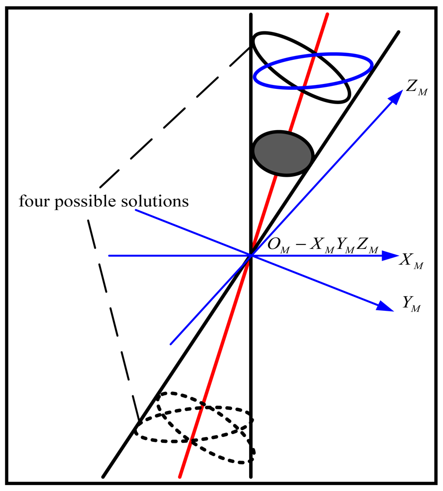
We focus on calibrating the relative pose between the perspective camera and the mirror. First, we use the ellipse-shaped mirror boundary image to estimate the four possible mirror postures based on Chen's extrinsic calibration method [18]. In order to remove the ambiguity of mirror posture, we then present a novel selection method making use of the imaged lens boundary to find the correct solution. Experiments conducted both on simulated data and real images confirm the performance of the proposed method.
In the following section the general model of non-central camera is briefly explained. After giving the algorithm idea in Section 3, Sections 4, 5, and 6 describe the three main steps of our algorithm in detail. Experimental results both on simulated data and real image are represented in Section 7. Finally, conclusions are given in the last section.
2. Camera Model
2.1. General Configuration of the Camera System
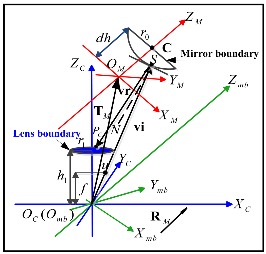
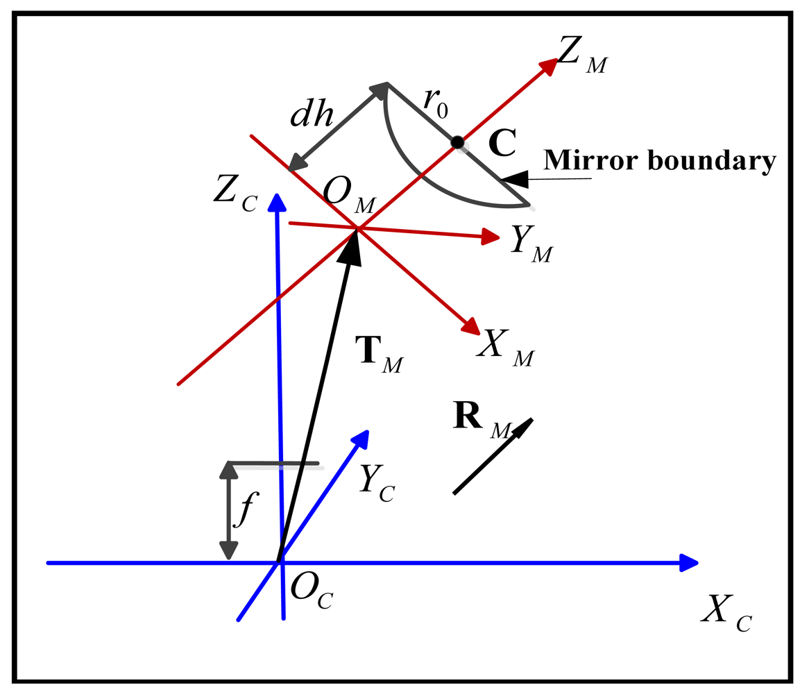
Figure 1 shows the general configuration of a catadioptric camera system, where the camera and the mirror coordinate systems are denoted with the subscripts “C” and “M” respectively. Due to the misalignment the rigid body transformation between the two coordinate systems, i.e., the rotation RM and translation TM, drifts from the ideal configuration and makes the system non-central.
The full model of the non-central system should include the parameters of the mirror and the conventional perspective camera as well as the relative posture between the mirror and the camera. Generally the manufacture of the mirror can be fairly accurate and the deviation from the theoretic design could be very small. Meanwhile the intrinsic parameters of the perspective camera can also be computed in advance by some mature algorithms like the calibration toolbox from Jean-Yves Bouguet [19], and they do not change when misalignment of catadioptric system happens. Therefore we believe it is reasonable and valuable to find a good self-calibration method by computing the relative posture between the mirror and camera given their intrinsic parameters.
2.2. Perspective Camera Model
Let XC = (XC,YC,ZC)T be the coordinates of a 3D point in the camera coordinate system and ũ=(u,v,1)T be the homogenous coordinates of the image point respectively, according to the pinhole model we have:
3. Algorithm Idea
The idea of the calibration algorithm will now be described. Before calibration a calibrating image should be acquired from the catadioptric camera. Different from most of the existing calibration methods, there is no any special calibration pattern in the environment. The only requirement for the image is the mirror boundary and the lens boundary or at least part of them should be clearly visible in the image, which is true for most of the catadioptric cameras. Now it is required to determine the mirror posture relative to the camera coordinate system. The steps of the algorithm are as follows.
Image preprocessing and robust ellipse extracting. The images of the mirror and lens boundary can be extracted and fitted with ellipses, which actually encodes the mirror posture (Section 6).
Mirror posture computing based on the imaging ellipse of the mirror boundary. It is a non-iterative method and finally two posture candidates are obtained (Section 4).
Correct posture selecting based on the image of lens boundary. During the selection process, the unknown position of the real lens boundary relative to the optical center should also be estimated simultaneously (Section 5).
The steps of this algorithm will be described in detail in the subsequent sections of the paper. The main subject of this paper comprises the last two steps of this algorithm, which will be described first. The first step is of peripheral interest, and a description of the robust method used for automatic ellipse extracting and fitting will be postponed to a later section.
4. Computing Mirror Posture Candidates
As show in Figure 1, the mirror posture can actually be represented by the transformation between the camera coordinate system OC − XCYCZC and the mirror coordinate system OM − XMYMZM. With intrinsic parameters of the perspective camera in hand, the next step is to compute the possible solutions of mirror postures by using the image of the mirror boundary. We apply Chen's method [18] to accomplish this. Considering a camera coordinate system OC − XCYCZC that the origin OC is the optical center and the ZC-axis is the optical axis asshown in Figure 1, the imaged mirror boundary can be described as an ellipse with the following form:
The quadratic form of Equation (3) is:
Substituting ũ in Equation (4) by Equation (1), an oblique ellipse cone in the camera coordinate system is obtained as follows:
As shown in Figure 1, a mirror boundary coordinate system Omb − XmbYmbZmb (the subscript “mb” stands for “mirror boundary”) is defined where the origin Omb overlapswith the optic center OC and Zmb-axis parallel with the unitnormal vector of the supporting plane of the circle to beviewed. The circle of mirror boundary centered at Cmb=(x0, y0, z0)T on Zmb=Z0 plane with known radius r0 can be described as:
Based on the definition of the two coordinate systems, only a rotation RM exists between the camera and mirror boundary coordinate system and the relationship can be expressed as:
To solve the above equation, first we convert Qc into a diagonal matrix by eigenvalue decomposition:
And from Equations (12), (13) and (14), the rotation from the mirror boundary coordinate to the camera coordinate is:
Finally we can describe the center of the circle and unit normal vector of the supporting plane in the camera coordinate system by the following expression:
In the mirror coordinate system OM − XMYMZM, being the central symmetric axis of the mirror, the ZM-axis is parallel to the vector nC while the origin OM does not overlap with the optical center. The translation between the mirror and the camera coordinate system is obtained by Equation (17), where dh is the distance from the mirror boundary center to OM.
Constraining nC points back towards the camera and CC lies in front of the camera as follows:
5. Mirror Pose Selection
Obviously more constraints are necessary to finally select the correct solution from the obtained posture candidates. In order for the calibration method to be independent of any special designed calibration patterns, we propose a novel method to achieve this by using the image of the lens boundary.
In the calibrating image, the lens boundary of the camera can also be easily observed in the center part of the image. The observed lens boundary in the image, whose size and position depends on the posture and the shape of the mirror, can be represented by a closed curve. Normally the curve is difficult to describe strictly by some special type of conics. For the revolutionary symmetric mirrors used in the catadioptric system, we find fitting the curve into an ellipse is accurate enough for the pose selection purpose, as we will see in the experiments. Theoretically, given the 3D position and the size of the lens boundary in the camera coordinate system, the correct posture can be selected by checking the similarity between the “observed” and the “predicted” lens boundary. There are two ways to define the “observed” and the “predicted” boundaries, each of which corresponds to checking the similarity under 2D image plane or 3D camera coordinate. In the 2D image plane, the “observed” one is the real ellipse we obtained and the “predicted” one is an ellipse computed by projecting the lens reflection on the mirror to the image plane. That is what our previous work has done [20] and it needs to calculate the reflective point on the mirror for each point on the lens boundary. The calculation has to be finished by a nonlinear optimization process and is very time-consuming. Here we propose a better way to check the similarity, where the “observed” is the real lens boundary in 3D camera coordinate and the “predicted” is the intersecting curves of a “cutting plane” with the reflective “cone” composed of the incident rays from the lens boundary. The “cutting plane” is actually the plane where the lens boundary lies in the camera coordinate system. For each pixel in the imaged lens boundary, the corresponding mirror points can be computed straightly and consequently the reflective “cone” can be obtained. Therefore this algorithm is much more effective.
However, in practice not all of the parameters of the lens boundary are known. Among those unknown the most important are the position parameters. Only the radius of the lens boundary can be found in the data sheet of the lens. By reasonably assuming the plane where the lens boundary lies be parallel with the X-Y plane of the camera coordinate system, the distance of the plane to the optical center is still left as an unknown. Therefore we need to estimate the distance of the lens boundary and select the correct mirror posture solution simultaneously.
Apparently this selection method can be applied to any type of the mirror as long as the mirror parameters are known. For simplicity we take the common hyperboloidal mirror as an example to explain the computing process.
The hyperboloidal mirror can be expressed by Equation (19):
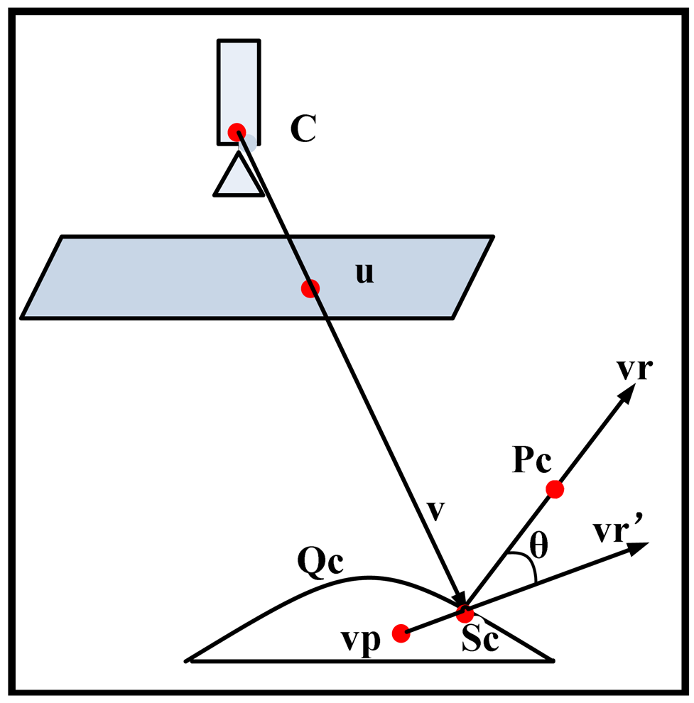
Given the mirror parameter , the next step is to obtain a reflective cone emitting from the mirror corresponding to the image of lens boundary. Due to the nonlinearity of the mirror shape, it's difficult to obtain a linear matrix form for the reflective cone. However as shown in Figure 3, the cone can be represented by a set of discrete reflective rays vr emitting from the mirror pointS, where each ray vrij corresponds to a sampling point uj(j = 0,1,2,…,n) in the imaged lens boundary.
In camera coordinates, from the perspective projection model, we have:
Expanding Equation (25) yields a quadric equation about λ. By imposing a positive depth constraint the correct root λ0 can be selected from the solution and hence can be determined. The normal vector to the quadric mirror at the reflective point is given by the first three coordinates of the tangent plane . The normalized normal vector is thus given by:
Now we have two set of rays vrij(i=1,2; j=1,2,…,n) which represent two reflective cones corresponding to the two posture candidates respectively. As shown in Figure 3, the lens boundary with radius r1 lies ahead of the optical center OC with distance h1. Two sets of intersecting points can be obtained by intersecting the rays vrij with the “cutting plane” at a distance h1 to OC. Writing and , can be computed by Equation (28):
Taking h1 as an unknown variable, one dimensional searching on h1's supporting region could be carried out. For each possible combination of posture labeled i and h1, one set of can be obtained by Equation (28). The set of the points can be fitted into an ellipse whose center and the length of the major axis a(i, h1) and minor axis b(i, h1) are all the functions of variables i and h1 and can all be computed, respectively. Obviously the correct i and h1 should result in a circle with radius r1 and central coordinates (0,0,h1)T. Therefore it is reasonable to construct an error function E measuring the difference between the intersecting ellipse and the real lens boundary as follows:
In Equation (29) the first term and the second term of E represent the central position error and the radius error respectively. Finally, the correct i and h1 can be obtained byminimizing the function, that is:
The function E is difficult to differentiate analytically, therefore a derivative-free optimizer is preferred. The downhill simplex method is a good candidate for this type of optimization [21].
6. Robust Ellipse Extracting and Fitting
In order to estimate the mirror posture, ellipses of the mirror and lens boundaries in the image need to be extracted accurately. Given a calibrating image, we propose a robust method to finish the ellipse extraction task automatically. First the Canny operator is applied to obtain an edge image. Then by using two Regions of Interest (ROIs) where the mirror boundary and lens boundary should appear respectively, most of the edge pixels outside the ROIs are removed. Meanwhile edge pieces with small length are also deleted from the image. After that, we do iterative least mean square ellipse fitting to all the remaining pixels within each ROI until convergence. As can be seen from Figure 10, the ideal mirror and lens boundary in the image appear to be the outmost and inmost elliptical contour. For mirror boundary, the initial fitted ellipse always sits inside the real boundary due to the existence of non-boundary pixels. Therefore during each iteration those edge pixels staying inside the fitted ellipse are removed so as to “expand” the fitted ellipse in the next iteration. A similar process is applied to the lens boundary except that a “shrinkage” strategy is used. The iteration continues until the fitting error is less than a threshold. To further improve the fitting accuracy, 5-point RANSAC ellipse fitting is applied to the rest edge pixels and the final optimal ellipse parameters can be obtained [22,23]. The advantage of this technique is that it can automatically extract the ellipse and obtain the ellipse parameters with high accuracy.
7. Experiments
To verify the proposed self-calibration method, some experiments based on simulation data and real images were carried out.
7.1. Experiment with Simulation Data
Based on the simulated camera configuration listed in Table 1, the synthesized imaging ellipses of the mirror and lens boundaries can be easily generated for calibration, respectively.
The calibration results are summarized in Table 2. They show that the calibration method is effective and the proposed selection method does find the correct pose solution and the height h1.
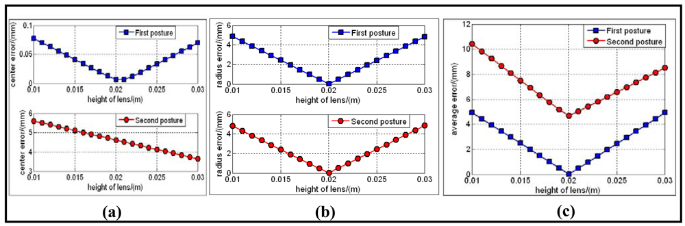
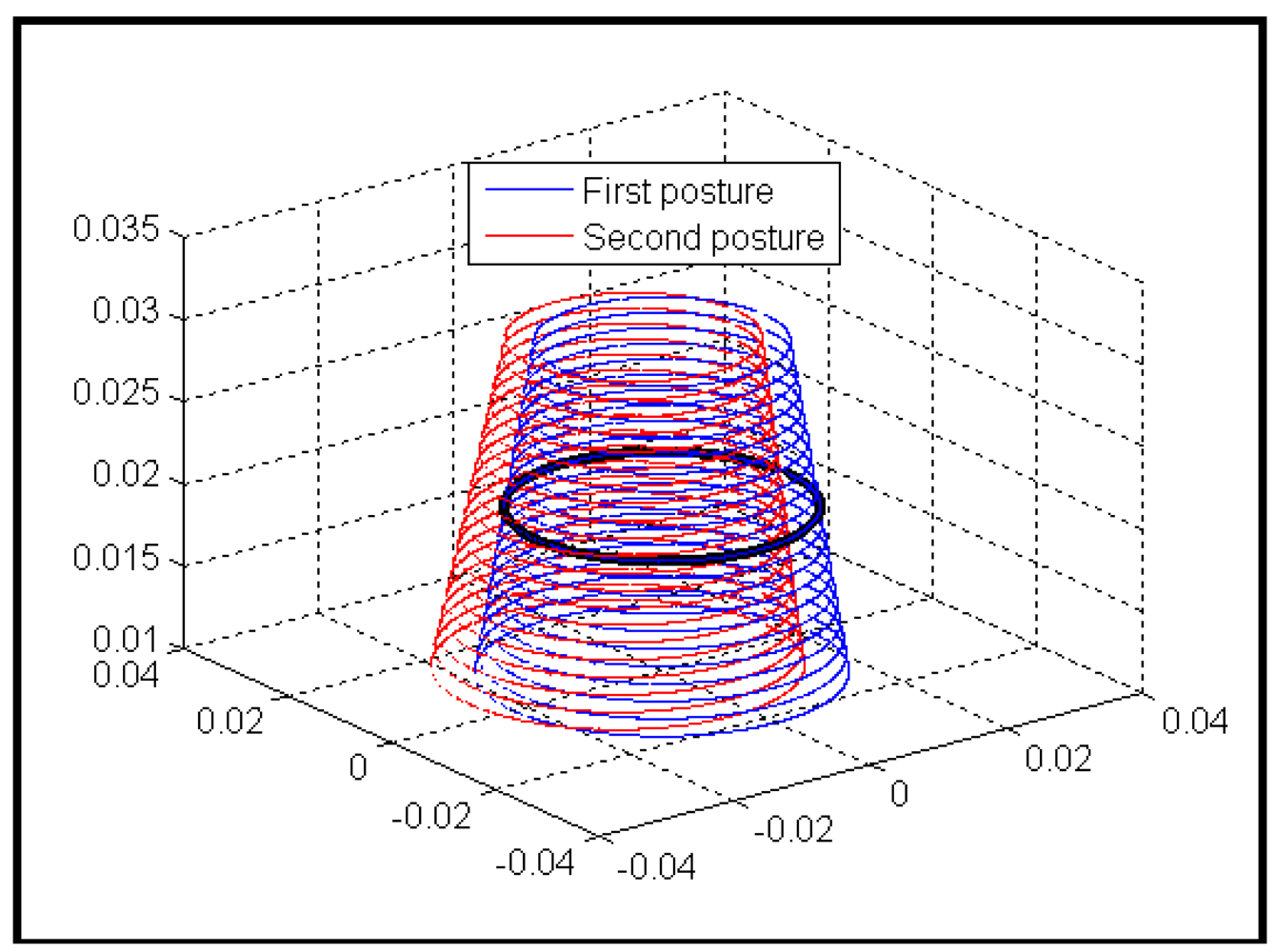
Figure 4 shows the typical variance of the position and the size of the two predicted lens boundaries with respect to the actual one within h1's supporting region. Figure 5(a–d) shows the central error, radius error, and combined average error between the predicted and the actual lens boundary respectively. From the two figures we can confirm that the minimum average error is reached when h1 is near 0.02 m, and the correct pose solution has been selected out.
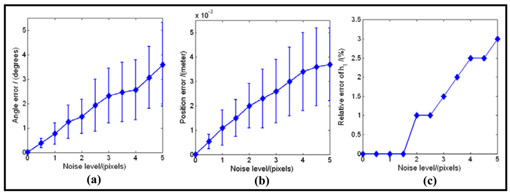
The results listed in Table 2, Figures 4 and 5 did not consider the noises which usually exist in the process of the boundary imaging, edge extraction and ellipse fitting. To see the robustness of the calibration method in the presence of noise, we added zero-mean Gaussian noise with standard deviation σ to the sampled points on the image of mirrorboundary and lensboundary. σ varies from 0 to 5 pixels in 0.5 pixel steps. For each noise level, the mirror posture and h1 areestimated by our algorithm. The difference between the estimated parameters and the ground truth were recorded as an error measurement. The resulting error of nC (angles, unitin degree), the error of CC (Euclidean distance, unit in meters) and the relative error of the detected h1 are shownin Figure 6. In all of the test cases, the calibration algorithm produced stable posture choices and the solution closer to the ground truth was correctly found. The results show that the proposed algorithm is robust in the condition of different noise levels.
7.2. Experiment with Real Images
7.2.1. Catadioptric Camera Setup
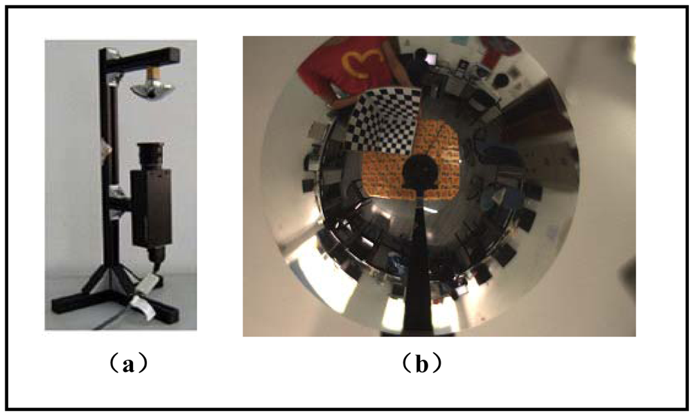
The catadioptric camera system we used for real data experiment is made by NEOVISION and is shown in Figure 7. It consists of a H3S hyperbolic mirror and a Sony XCD-SX910CR camera and was originally made as a central single viewpoint camera. More specifications of the system are listed in Table 3.We deliberately changed the relative position between the mirror and the camera, making it bias from the factory configuration. Therefore it was not a central camera again and actually became a new non-central catadioptric system. The intrinsic parameters of the conventional camera XCD-SX910CR are listed as follows: fx = 1455.07, fy = 1459.51, ks = 0, u0 = 639.2, v0 = 482.2, the image resolution is 1,280 × 960. The radius of the lens boundary is: r1=0.0185m.
7.2.2. Ellipse Extracting and Fitting Results
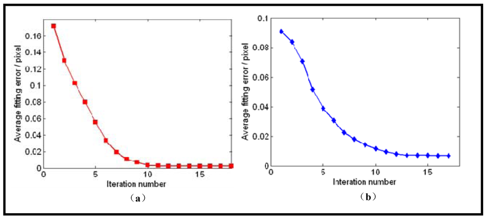
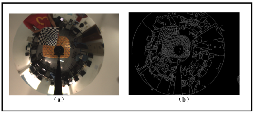
Figure 8 shows the calibration image and its canny detection result. Figure 9(a,b) shows the average fitting error of two boundaries with respect to the iteration number, respectively. It demonstrates that our iterative ellipse fitting process can refine the boundaries and quickly leads to convergence.
After using the remaining edge pixels for 5-point RANSAC, we get the final extracted and fitted ellipses, as shown in Figure 10. The ultimate average fitting errors of mirror and lens boundaries are 0.0022 and 0.0071 pixels, respectively.
7.2.3. Real Image Calibration
As we have the ellipse parameters of the mirror and the lens boundaries in hand, we apply our calibration algorithm to Figure 10. The final solution obtained is listed in Table 4. The resulting combined error between the actual and predicted lens boundary was 2.263 mm, which is very satisfying considering the existence of imaging noises.
7.3. Applications
7.3.1. Image Transformation
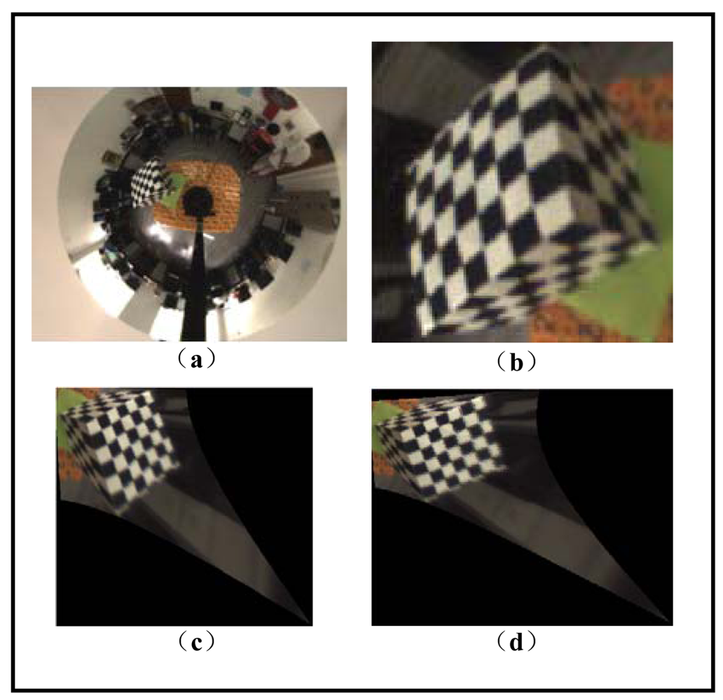
In this section, we evaluate the performance of our calibration method by image transformation. Since our catadioptric camera system does not maintain the single viewpoint characteristic, we cannot transform the whole omnidirectional image into a perspective one, but it is still possible to transform a patch of acquired image by assuming an approximate single viewpoint.
As shown in Figure 11, we try to find a virtual single viewpoint vp by minimizing the sum of the angle error between each real ray vr and the virtual ray vr' originated from the viewpoint vp, as expressed in Equation (31):
7.3.2. 3D Reconstruction
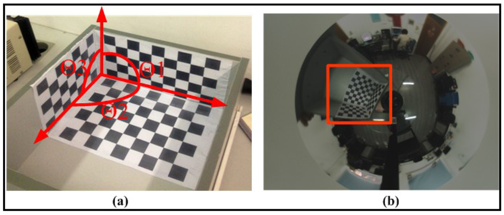
To further verify the performance of our calibration algorithm quantitatively, we employed a trihedral object composed of three orthogonal checker patterns of known size (Figure 13(a)) and computed the angles between normal vectors of each checkerboard plane. First a sub-image containing the trihedral object was transformed into a perspective one using the method described above. Then a traditional camera calibration toolbox [19] was used to compute the normal directions of the three checkerboard planes respectively. Finally the three angles Θ1, Θ2 and Θ3, as shown in Figure 13(a) can be obtained.
Two different non-central configurations are designed for the experiment. The first configuration is denoted as “slightly non-central” which means the mirror focus is only biased a little from the ideal position. The second configuration is denoted as “medium non-central” which has several centimeters in the translation and several degrees in the rotation away from the ideal case. The posture parameters from the default factory configuration, Mei's calibration method [24] and our method are used for computing the angles, respectively. In each configuration 10 images with the trihedral object at different positions around the camera are acquired and the average values of the computed angles are recorded in Table 5. The three angles should all be 90 degrees in an ideal situation. From the table, we can see that angles calculated from our calibration algorithm are better than results from the default factory configuration in both configurations. For the slightly non-central case the results from our method and Mei's are comparable, while for the second case our method shows superior performance than Mei's. The reason is Mei's method is only designed for the central camera while our method can deal with the central and non-central situation equally.
8. Conclusions
A novel self-calibration method for non-central catadioptric cameras is proposed in this paper. We use the mirror boundary in the image to obtain the possible mirror posture candidates, and then select the correct solution by using the image of the lens boundary. In the implementation stage we also presented a robust ellipse extraction algorithm based on iterative outlier rejection followed by RANSAC. Both the computer simulation and real data have been used to test the proposed technique, and very satisfying results have been obtained. The calibration method is not subject to the constraint of slightly non-central misalignment and is able to calibrate the non-central camera in a single image using only the catadioptric camera itself. This also makes the method qualified for on-the-fly calibration processes and is particularly beneficial for the situation where no calibration patterns are available, such as off-road and planet robot navigation.
Acknowledgments
This research work is supported by National Science Foundation of China (NSFC) 61071219 and the Fundamental Research Funds for the Central Universities.
References
- Nayar, S.K. Catadioptric Omnidirectional Camera. Proceedings of IEEE Computer Society Conference on Computer Vision and Pattern Recognition, San Juan, Puerto Rico, 17–19 June 1997; pp. 482–488.
- Fernando, C.G.; Munasinghe, R.; Chittooru, J. Catadioptric Vision Systems: Survey. Proceedings of the Thirty-Seventh Southeastern Symposium on System Theory, Tuskegee, AL, USA, 20–22 March 2005; pp. 443–446.
- Agrawal, A.; Taguchi, Y.; Ramalingam, S. Beyond Alhazen's Problem: Analytical Projection Model for Non-Central Catadioptric Cameras with Quadric Mirrors. Proceedings of IEEE Conference on Computer Vision and Pattern Recognition, Colorado Springs, CO, USA, 21–23 June 2011; pp. 2993–3000.
- Srinivasan, M.V. A New Class of Mirrors for Wide-Angle Imaging. Proceedings of the 2003 Conference on Computer Vision and Pattern Recognition Workshop, Madison, WI, USA, 16–22 June 2003; Volume 7. pp. 85–90.
- Swaminathan, R.; Grossberg, M.; Nayar, S. Non-Single Viewpoint Catadioptric Cameras: Geometry and Analysis. Int. J. Comput. Vision 2006, 66, 211–229. [Google Scholar]
- Micusik, B.; Pajdla, T. Autocalibration & 3D Reconstruction with Non-Central Catadioptric Cameras. Proceedings of the IEEE Computer Society Conference on Computer Vision and Pattern Recognition, Washington, DC, USA, 27 June–2 July 2004; Volume 1. pp. 58–65.
- Grossberg, M.D.; Nayar, S.K. The Raxel Imaging Model and Ray-Based Calibration. Int. J. Comput. Vision 2005, 61, 119–137. [Google Scholar]
- Morel, O.; Fofi, D. Calibration of Catadioptric Sensors by Polarization Imaging. Proceeding of IEEE International Conference on Robotics and Automation, Roma, Italy, 10–14 April 2007; pp. 3939–3944.
- Ainouz-Zemouche, S.; Morel, O.; Mosaddegh, S.; Fofi, D. Adapted Processing of Catadioptric Images Using Polarization Imaging. Processing of 16th IEEE International Conference on Image, Cairo, Egypt, 7–11 November 2009; pp. 217–220.
- Fabrizio, J.; Tarel, J.; Benosman, R. Calibration of Panoramic Catadioptric Sensors Made Easier. Proceeding of Third Workshop on Omnidirectional Vision, Washington DC, USA, 2 June 2002; pp. 45–52.
- Goncalves, N.; Araujo, H. Projection Model, 3D Reconstruction and Rigid Motion Estimation from Non-Central Catadioptric Cameras. Processing of 2nd International Symposium on 3D Data, Visualization and Transmission Conference, Thessaloniki, Greece, 6–9 September 2004; pp. 325–332.
- Mashita, T.; Iwai, Y.; Yachida, M. Calibration Method for Misaligned Catadioptric Camera. IEICE Trans. Inform. Syst. 2006, E89 (D), 1984–1993. [Google Scholar]
- Kang, S.B. Catadioptric Self-Calibration. Proceedings of the Conference on Computer Vision and Pattern Recognition, Hilton Head, SC, USA, 13–15 June 2000; Volume 1. pp. 201–207.
- Stelow, D.; Mishler, J.; Koes, D.; Singh, S. Precise Omnidirectional Camera Calibration. Proceedings of IEEE Conference on Computer Vision and Pattern Recognition, Kauai, HI, USA, 8–14 December 2001; Volume 1. pp. 689–694.
- Goncalves, N.; Araujo, H. Estimating Parameters of Noncentral Catadioptric Systems Using Bundle Adjustment. Comput. Vision Image Understand. 2009, 113, 1–28. [Google Scholar]
- Caglioti, V.; Taddei, P.; Boracchi, G.; Gasparini, S.; Giusti, A. Single-Image Calibration of Off-Axis Catadioptric Cameras Using Lines. Proceedings of IEEE 11th International Conference on Computer Vision, Rio de Janeiro, Brazil, 14–20 October 2007; pp. 1–6.
- Agrawal, A.; Taguchi, Y.; Ramalingam, S. Analytical Projection for Axial Non-Central Dioptric and Catadioptric Cameras. Proceedings of 11th European Conference on Computer Vision, Crete, Greece, 5–11 September 2010; Volume 6313. pp. 129–143.
- Chen, Q.; Wu, H.; Wada, T. Camera Calibration with Two Arbitrary Coplanar Circles. Proceedings of European Conference on Computer Vision, Washington DC, USA, 27 June–2 July 2004; Volume 3. pp. 521–532.
- Bouguet, J.Y. Camera Calibration Toolbox for Matlab. Available online: http://www.vision.caltech.edu/bouguetj/calib_doc/ (accessed on 7 January 2012).
- Fitzgibbon; Pilu, M.; Fisher, R. Direct Least Square Fitting of Ellipses. IEEE Trans. Patt. Anal. Mach. Intell. 1999, 21, 476–480. [Google Scholar]
- Fischler, M.A.; Bolles, R.C. Random Sample Consensus: A Paradigm for Model Fitting with Applications to Image Analysis and Automated Cartography. Commun. ACM 1981, 24, 381–395. [Google Scholar]
- Xiang, Z.; Sun, B. A Novel Self-Calibration Method for Non-Central Catadioptric Camera System. Processing of the Third IEEE International Conference on Intelligent Computing and Intelligent Systems, Guangzhou, China, 24–26 October 2011; Volume 1. pp. 735–739.
- Press, W.H.; Vetterling, W.T.; Teukolsky, S.A.; Flannery, B.P. Numerical Recipes in C: The Art of Scientific Computing, 2nd ed.; Cambridge University Press: Cambridge, UK, 1997. [Google Scholar]
- Mei, C.; Rives, P. Single View Point Omnidirectional Camera Calibration from Planar Grids. IEEE International Conference on Robotics and Automation, Roma, Italy, 10–14 April 2007; pp. 3945–3950.


| Intrinsic Parameters | Focal Length (pixel) | fx = fy = 1500 |
| Skew Coefficient | ks = 0 | |
| Principal Points | u0 = 640, v0 = 480 | |
| Mirror Parameters | Mirror Boundary radius (m) | r0 = 0.028 |
| Major axis (m) | am = 0.028 | |
| Minor axis (m) | bm = 0.023 | |
| Lens Parameters | Lens Boundary radius (m) | r1 = 0.018 |
| Height From Optical (m) | h1 = 0.02 | |
| Mirror Posture | Mirror Center to O M (m) | dh = 0.0425 |
| Normal vector | nC=(0.0349, −0.0523, 0.9980)T | |
| Mirror Center (m) | CC=(0.0002, 0.0005, 0.083)T | |
| Parameters | Solution |
|---|---|
| Mirror Center CC (m) | CC1=(0.0002, 0.0005, 0.0830)T, CC2=(0.0008, −0.0005, 0.0830)T |
| Translation TM (m) | TM1=(−0.0013, 0.0027, 0.0406)T, TM2=(0.0017, −0.0027, 0.0406)T |
| Rotation RM | |
| Height h1 (m) | h1=0.02 |
| Calibration Result | TM1,RM1,h1 |
| Type | hyperbolic | 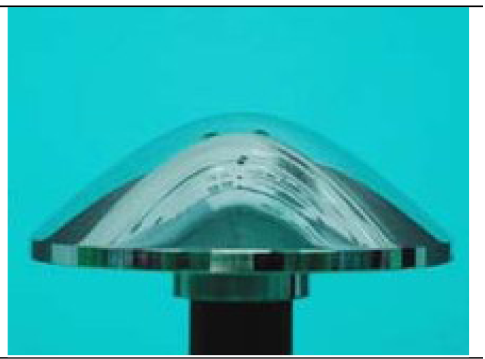 |
| Major Axis | 28.0950 mm | |
| Minor Axis | 23.4125 mm |
| Parameters | Solution |
|---|---|
| Mirror Center CC (m) | CC = (0.0012, −0.0060, 0.0796)T |
| Translation TM (m) | TM = (0.0002, −0.0065, 0.0339)T |
| Rotation RM | |
| Height h1 (m) | h1 = 0.013 |
| Methods | Slightly non-central/degrees | Medium non-central/degrees | ||||
|---|---|---|---|---|---|---|
| Θ1 | Θ2 | Θ3 | Θ1 | Θ2 | Θ3 | |
| Factory Configuration | 85.37 | 96.58 | 83.65 | 93.41 | 107.99 | 91.33 |
| Mei's Method | 87.65 | 91.12 | 88.70 | 92.01 | 62.54 | 65.25 |
| Our Method | 88.10 | 92.31 | 89.06 | 89.98 | 89.36 | 91.07 |
© 2012 by the authors; licensee MDPI, Basel, Switzerland. This article is an open access article distributed under the terms and conditions of the Creative Commons Attribution license (http://creativecommons.org/licenses/by/3.0/).
Share and Cite
Xiang, Z.; Sun, B.; Dai, X. The Camera Itself as a Calibration Pattern: A Novel Self-Calibration Method for Non-Central Catadioptric Cameras. Sensors 2012, 12, 7299-7317. https://doi.org/10.3390/s120607299
Xiang Z, Sun B, Dai X. The Camera Itself as a Calibration Pattern: A Novel Self-Calibration Method for Non-Central Catadioptric Cameras. Sensors. 2012; 12(6):7299-7317. https://doi.org/10.3390/s120607299
Chicago/Turabian StyleXiang, Zhiyu, Bo Sun, and Xing Dai. 2012. "The Camera Itself as a Calibration Pattern: A Novel Self-Calibration Method for Non-Central Catadioptric Cameras" Sensors 12, no. 6: 7299-7317. https://doi.org/10.3390/s120607299