A Rank-Ordered Marginal Filter for Deinterlacing

Abstract

This paper proposes a new interpolation filter for deinterlacing, which is achieved by enhancing the edge preserving ability of the conventional edge-based line average methods. This filter consists of three steps: pre-processing step, fuzzy metric-based weight assignation step, and rank-ordered marginal filter step. The proposed method is able to interpolate the missing lines without introducing annoying articles. Simulation results show that the images filtered with the proposed algorithm restrain less annoying pixels than the ones acquired by other methods.

1. Introduction

Interlaced scanning has been advanced from the early days of TV and still adopted for SDTV and 1080i HDTV broadcast standards [1]. However, nearly all late model flat panel displays (LCD, PDP, etc.) use progressive scanning formats. For these display devices, an entering interlaced video signal has to be transformed to a progressive one, and thus a scanning format conversion that gives compatibility between various video formats is required [2]. The super-resolution (SR) is a class of techniques that enhance the resolution of an imaging system [3–8]. The deinterlacing only considers vertical direction, while SR considers both of vertical and horizontal directions. Thus, the intra-field deinterlacing is a special case of SR.

Many deinterlacing methods have been proposed, including spatial methods [9–13] and motion-based methods [14]. Although motion-based methods yield better subjective quality than spatial methods, they require reliable motion models and the estimated trajectories must be sufficiently proper, which generally causes excessive computational complexity On the other hand, spatial methods have lower computational complexity since they only demand the current frame, making them more suitable for real-time applications. Therefore, in this paper, we focus on the spatial method.

Among spatial approaches, deinterlacing based on edge direction is the most outstanding and broadly adopted method. These methods calculate edge information first and then decide edge direction to utilize appropriate pixels for interpolation. Thus the edge information calculation and edge direction decision are the key steps. However, conventional methods have yielded poor performance when edge direction is not credible.

To shorten this issue, we propose a deinterlacing algorithm using rank-ordered fuzzy metric approach to reduce artifacts in deinterlaced images. In our approach, the missing lines are calculated by weight obtained using fuzzy metric (FM) from the existing neighbor pixels. The local FM infers the weight of the edge information. Thus, we deinterlace the interlaced signal without calculating edge directions as the traditional approaches do. After that, the rank-ordered differences statistic introduced in [15] is accommodated to the fuzzy context utilizing the introduced FM.

The paper is arranged as follows. Section 2 introduces FM used in the weight assignation step. After that, the proposed filtering technique is described. Section 3 shows simulation results including performance comparison and computational complexity. Finally, conclusions are drawn in Section 4.

2. Proposed Method

2.1. Fuzzy Metric for Weight Assignment

A stationary FM, on a set S, is a fuzzy set of S × S satisfying the following conditions for all p,q,r ∈ S[15]:

• Rule₁: FM_s(p,q,t) > 0;

• Rule₂: FM_s(p, q, t) = 1 if and only if p = q;

• Rule₃: FM_s(p,q,t) = FM_s(q,p,t);

• Rule₄: FM_s(p, q, t) ≥ FM_s(q, r, u) * FM_s(p, r,t + u);

where Rule_# is a FM of rule number #, * is a continuous t-norm, FM_s(p, q, t) stands for the degree of nearness between p and q according to Rule₂, FM_s(p, q, t) is close to 0 when p is far from q. Let S be the set {0,1,…, 255}, then, the function FM : S × S → [0,1] given by

$$F{M}_S(p,q)={\left(\frac{\mathit{\text{min}}(p,q)+b}{\mathit{\text{max}}(p,q)+b}\right)}^a$$

(1)

where b is a small positive value for preventing max(p, q) = 0 singularity. As the difference between the components p and q become bigger, the value of FM_s falls quickly. Thus, we assume FM_s(p, q) is the fuzzy distance between the image components p and q. Clearly, FM is F-founded and it meets

$$0\le \frac{b}{I_{\mathit{\text{max}}}+b}\le F{M}_S(p,q)\le 1$$

(2)

for all p,q ∈ S, I_max is maximum pixel intensity, and I_max = 255 in this paper.

2.2. Deinterlacing Implementation

The proposed filter consists of three steps: (1) pre-processing step, (2) FM-based weight assignation step, and (3) rank-ordered marginal filter step. To begin with, we conduct interpolation with three missing pixels at location (−1, 0), (0, 0), and (1, 0), with vertical six-tap filters. After that, we evaluate FM degree using the introduced FM equation. The obtained FM degree is used for assigning weights. Finally, the missing pixel is calculated using the rank-ordered marginal filtering (ROMF) scheme.

Let us assume that I is an image and I(_c,_r) is the pixel intensity at a position of (c, r), c is column number and r is raw number, and I_(0,0) is the centered missing pixel to be processed. We denote W as a filtering window centered on the pixel under processing of size N×N,N = 3,5,7,…, which contains n = N² pixels. The pixels in W are symbolized as I(_c,_r), and c, r = −1, 0,1 for N = 3 case.

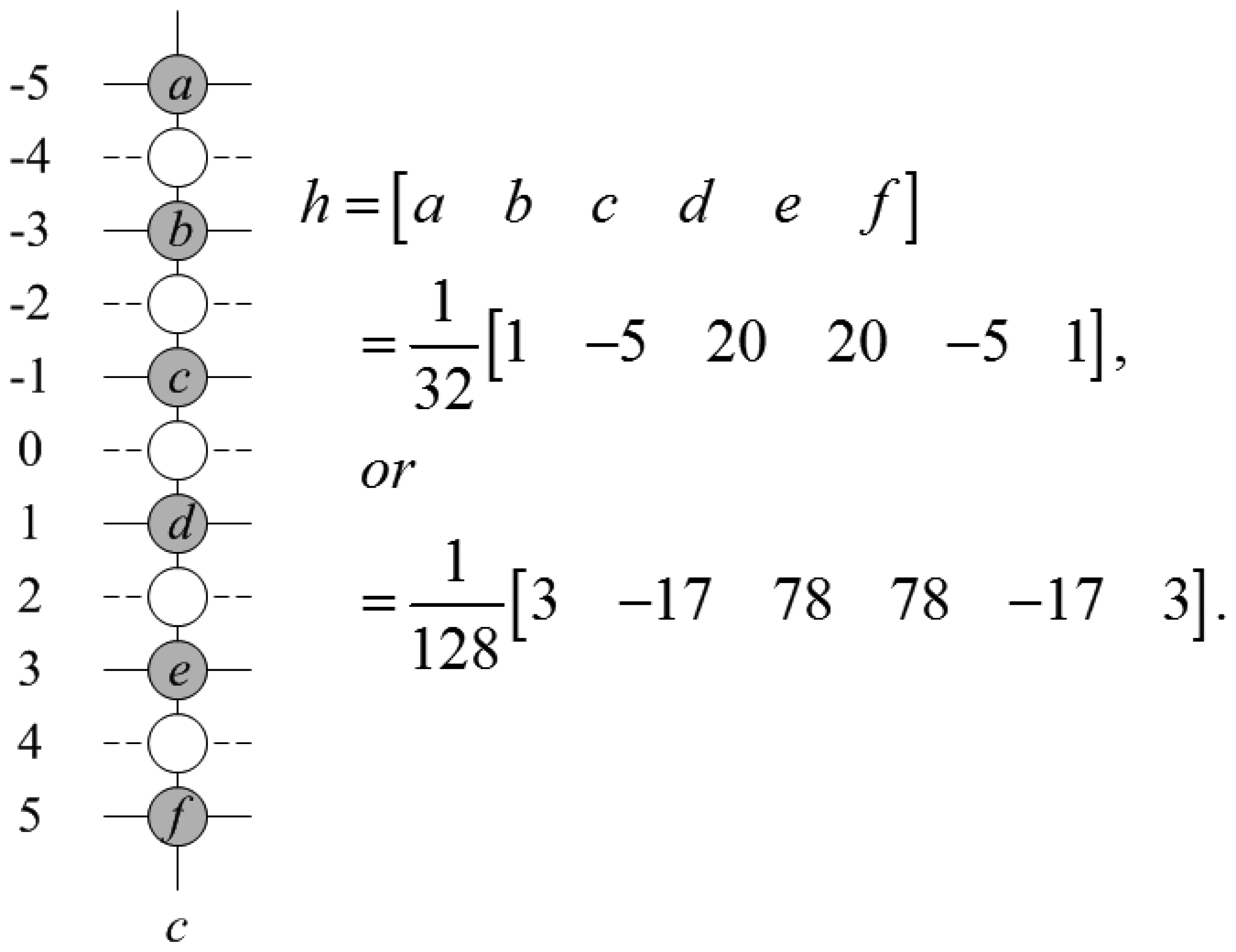
The first step of the ROMF method is vertical six-tap filter (STF). This fixed coefficient six-tap Wiener filter is widely used to estimate the sub-pixels in video codec, such as MPEG-4, H.264/AVC, and some deinterlacing methods [16]. The coefficients of this filter can be different such as h = [1, −5, 20, 20, −5, 1]/32 or h = [3, −17, 78, 78, −17, 3]/128. In this paper, we chose the previous one for our system under the assumption that h can calculate missing lines in the sub-pixel position properly. The missing pixels at (c, 0) position, c = −1,0,1, are estimated using the adjacent pixels at (c, −5), (c, −3), (c, −1), (c, 1), (c, 3), and (c,5), and we denote them as I(_c,₋₅), I_(c,−3), I_(c,−1), I_(c,1), I_(c,3), and I_(c,5), respectively. To interpolate the pixel more precisely, we must adapt the filter to accommodate the new interpolation condition. Now, three pixels in the missing line $I_{(-1,0)}^{\mathit{\text{STF}}}$, $I_{(0,0)}^{\mathit{\text{STF}}}$ and $I_{(1,0)}^{\mathit{\text{STF}}}$ are approximately deinterlaced applying Equation (3); however, they are not the same with the original missing pixel. Figure 1 shows the pixel positions with filter coefficients.

$$I_{(c,0)}^{\mathit{\text{STF}}}=h(1)I_{(c,-5)}+h(2)I_{(c,-3)}+h(3)I_{(c,-1)}+h(4)I_{(c,1)}+h(5)I_{(c,3)}+h(6)I_{(c,5)}$$

(3)

For the ROMF, eight neighboring pixels, I_(−1,−1), I_(0,−1), I_(1,−1), $I_{(-1,0)}^{\mathit{\text{STF}}}$, $I_{(1,0)}^{\mathit{\text{STF}}}$, I_(−1,1), I_(0,1) and I_(1,1) are employed to deinterlace the missing center pixel at (0,0). In this paper, we take FM_S as the distance function (note, however, that any other function such as Euclidean distance could be used). Therefore, the distance between two pixels $I_{(0,0)}^{\mathit{\text{STF}}}$ and I_(c,_r) is symbolized as FM_S ( $I_{(0,0)}^{\mathit{\text{STF}}}$,I_(c,_r)). We denote W̅ the set of neighbors of $I_{(0,0)}^{\mathit{\text{STF}}}$, that is, $\overline{W}=W-I_{(0,0)}^{\mathit{\text{STF}}}$.

The second step is to calculate eight FM using FM_s( $I_{(0,0)}^{\mathit{\text{STF}}}$, I_(c,_r)) where I_(c,_r) ∈ W̅. The proposed deinterlacing solves the problem by looking for the most robust I_(c,_r) pixel. To compute ROMF, the distance FM_S( $I_{(0,0)}^{\mathit{\text{STF}}}$,I_(c,_r)) are rearranged in an ascending order so that a group of non-negative real values χ_m, where fixed a positive integer m ≤ n − 1, are obtained. Note that χ_m is not always different: χ₁ ≤ χ₂ ≤ … ≤ χ_m ≤ … χ_n−1. Generally speaking, χ_j is the j^th smallest FM_S( $I_{(0,0)}^{\mathit{\text{STF}}}$,I_(c,_r)) value, and its associated I_(c,_r) is denoted as I_χj. Finally, the proposed ROMF calculates the missing pixel $I_{(0,0)}^{\mathit{\text{ROMF}}}$:

$$I_{(0,0)}^{\mathit{\text{ROMF}}}=\frac{1}{2}{I}_{(0,0)}^{\mathit{\text{STF}}}+\frac{1}{2}\frac{{\sum }_{j=-1}^m{\chi }_j\cdot I_{\chi j}}{{\sum }_{j=-1}^m{\chi }_j}$$

(4)

where χ_j is assumed to be a weight factor. It can be observed from Equations (1) and (4) that, when I_χj and $I_{(0,0)}^{\mathit{\text{STF}}}$ have similar values, the weight factor χ_j becomes large. On the other hand, when the difference between I_χj and $I_{(0,0)}^{\mathit{\text{STF}}}$ are large, χ_j becomes smaller. Thus, the missing line is deinterlaced based on the similarity among their neighbor pixels, I_χj, with allocated weights based on the FM.

3. Simulation Results

To evaluate the performance of the proposed algorithm, we present the simulation results in this section. We considered twenty images and video sequences as the dataset, which are shown in

Table 1. Test and training sets classified by alphabetical order.

Test images (I) and video (V) sequences (images starting with “A” to “G”):

Airplane (I), Akiyo (V), Barbara (I), Bluesky (V), Boat (I), Bus (V), City (V), Finger (I), Football (V), Girl (I)

Training images (I) and video (V) sequences (images start with “K” to “Z”):

Kimono (V), Lena (I), Man (I), Milkdrop (I), Mobile (V), News (V), Peppers (I), Raven (V), Toys (V), Zelda (I)

. The ten images starting with “A” to “G” are the test images, and the others (images starting with “K” to “Z”) are the training images.

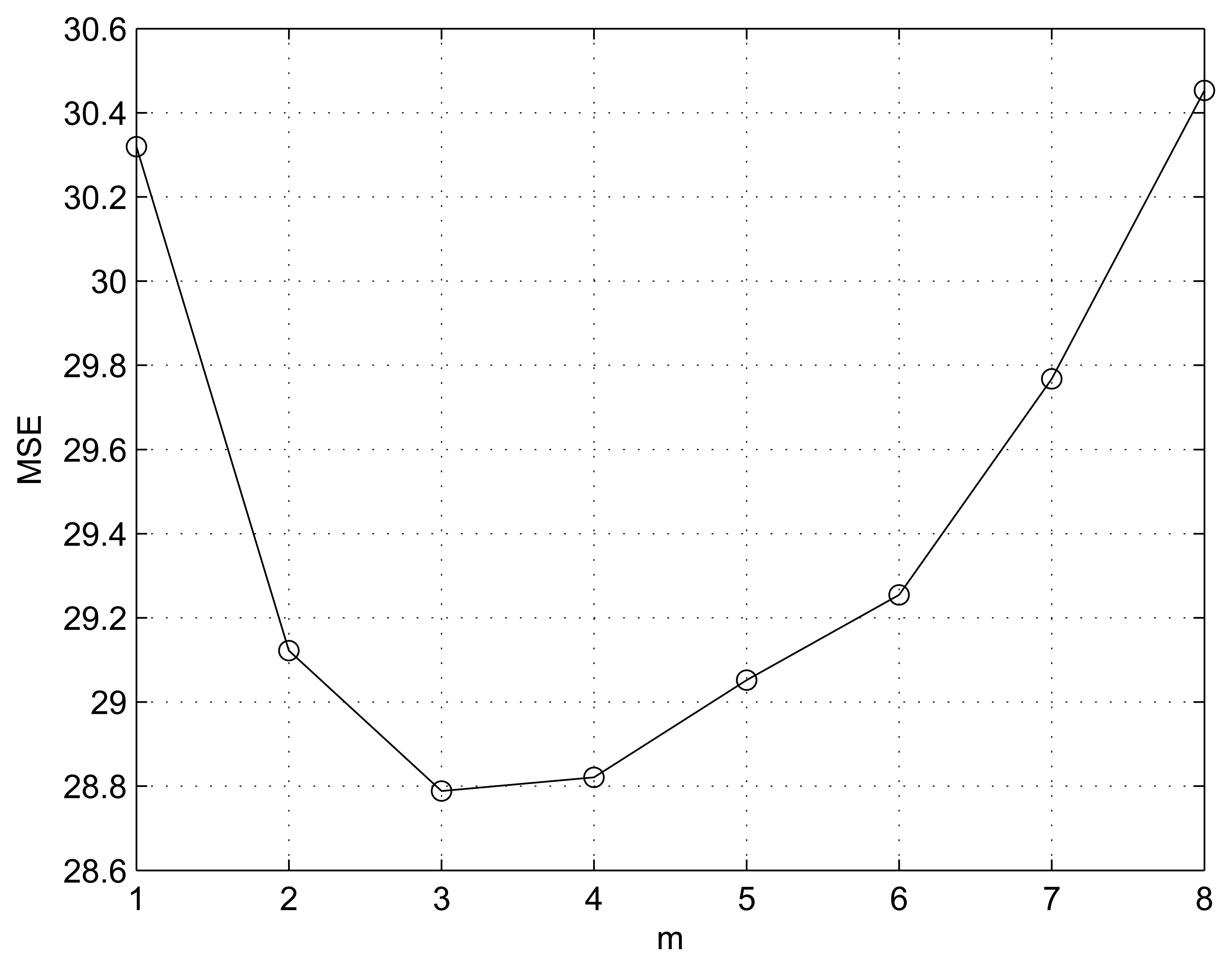
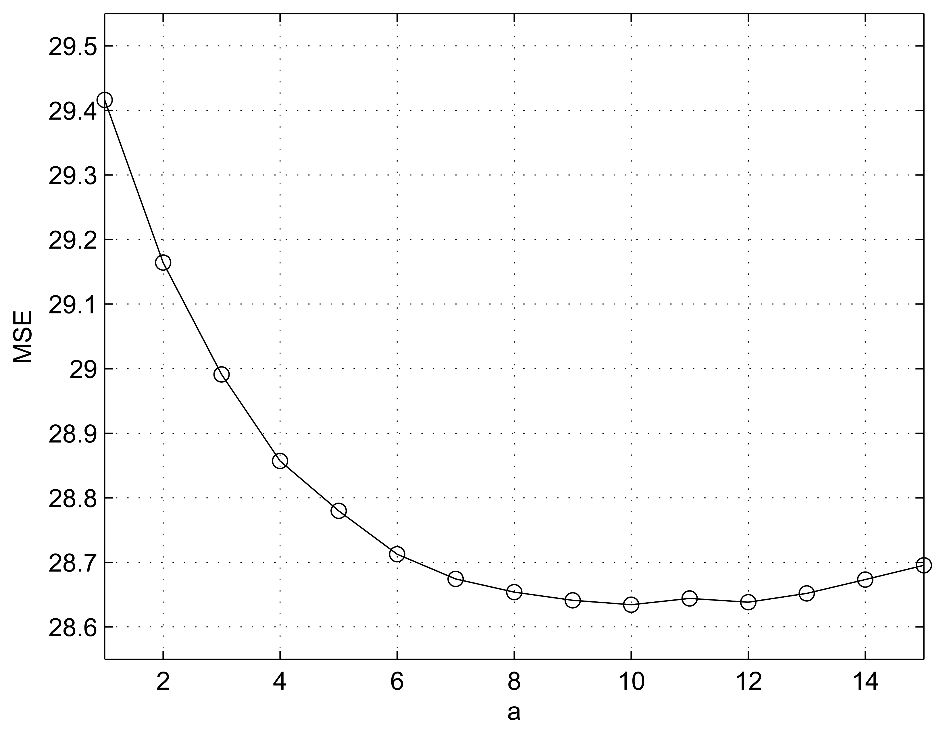
We conducted simulation using MATLAB with an Intel(R) Core(TM) i5 CPU M460 @ 2.53 GHz processor. We compared the proposed method with MELA [9], LABI [10], FEPD [11], MCAD [12] and LSMD [13] methods. Note that the designed filter parameters a and b and the number of considered neighbor pixels m play crucial roles, making it important to set them appropriately. One assumption is that, as we mentioned in Section 2, parameter b is a small positive value for avoiding max(p,q) = 0 singularity. Thus we gave b=1, which is the smallest intensity step. Figure 2 shows the average MSE performance of the proposed method according to various m values under the condition of b = 1 and 1 ≤ a ≤ 15. From Figure 2, m = 3 is determined to give the least MSE. Another parameter a = 10 is determined under the condition of b = 1 and m = 3, as shown in Figure 3.

The PSNR metric in decibels (dB) was selected to evaluate the performance.

Table 2. Comparison of the average PSNR for 10 test images and video sequences among different deinterlacing methods.

	MELA	LABI	FEPD	MCAD	LSMD	ROMF	Ranking
airplane	35.088	35.345	34.385	35.085	35.660	36.084	1
akiyo	40.205	38.841	37.255	39.726	38.149	40.098	2
barbara	32.018	31.930	28.879	25.929	29.414	33.562	1
bluesky	37.900	37.798	37.510	38.107	39.373	39.547	1
boat	35.186	35.277	33.074	35.342	33.762	36.034	1
bus	28.654	28.217	28.104	28.262	28.095	28.619	2
city	31.460	31.497	31.258	31.527	31.656	31.726	1
finger	31.323	31.362	30.679	31.810	32.085	32.946	1
football	35.057	34.475	33.308	35.034	34.763	35.791	1
girl	41.793	41.535	39.676	42.038	41.545	43.861	1
avg.	34.868	34.628	33.413	34.286	34.450	35.827	1

shows the comparison results of the PSNR performance of the proposed method to the benchmarks. After the experiments, it is obvious that the proposed method outperforms other methods by 0.959 (MELA), 1.199 (LABI), 2.414 (FEPD), 1.541 (MCAD), and 1.377 (LSMD) dB in terms of average PSNR. For Akiyo and Bus image, MELA showed a better PSNR performance of 0.107 dB and 0.035 dB. However, the proposed method showed the best PSNR performance for the other images.

Table 3. Comparison of the average CPU time for 10 test images and video sequences among different deinterlacing methods.

	MELA	LABI	FEPD	MCAD	LSMD	ROMF	Ranking
airplane	0.547	14.698	28.491	22.547	4.286	1.231	4
akiyo	0.207	5.694	10.947	7.861	1.838	0.596	4
barbara	0.490	14.154	29.527	20.609	4.409	0.787	4
bluesky	3.076	123.768	228.331	159.369	34.895	6.067	4
boat	0.470	13.490	28.727	20.191	4.076	1.107	4
bus	0.164	5.406	10.919	8.846	2.304	0.703	4
city	1.358	48.484	105.553	73.752	16.502	2.590	4
finger	0.397	12.349	29.005	20.315	4.036	1.057	4
football	0.203	5.057	12.676	7.755	1.668	0.794	4
girl	0.433	12.305	30.801	19.886	4.070	1.065	4
avg.	0.734	25.54	51.498	36.113	7.809	1.599	4

shows the CPU time per image. As we can see, the proposed method has more complexity than MELA. However, the proposed technique reduces the average CPU time up to 93.74%, 96.89%, 95.57%, and 79.52% when compared with LABI, FEPD, MCAD, and LSMD, respectively.

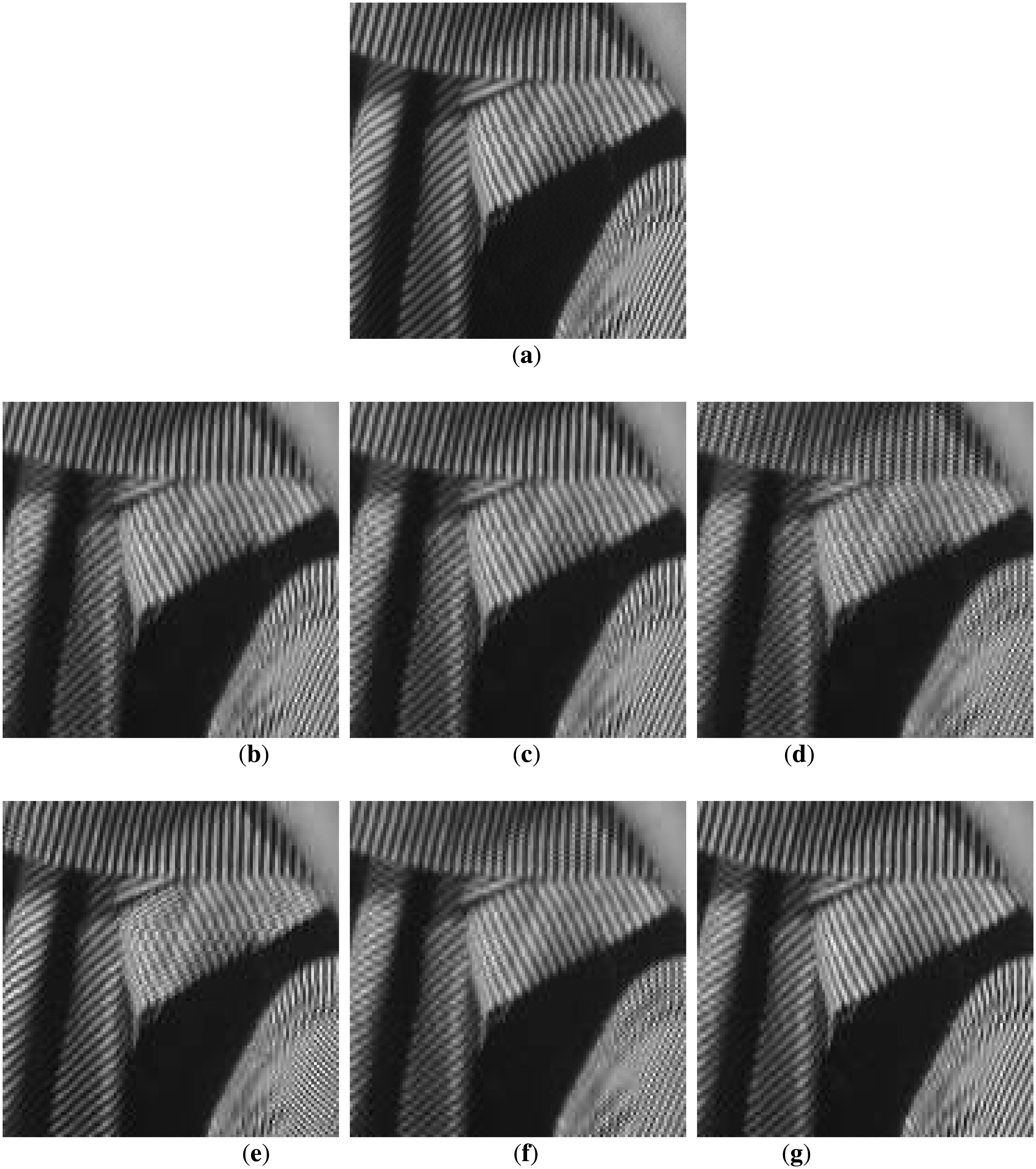
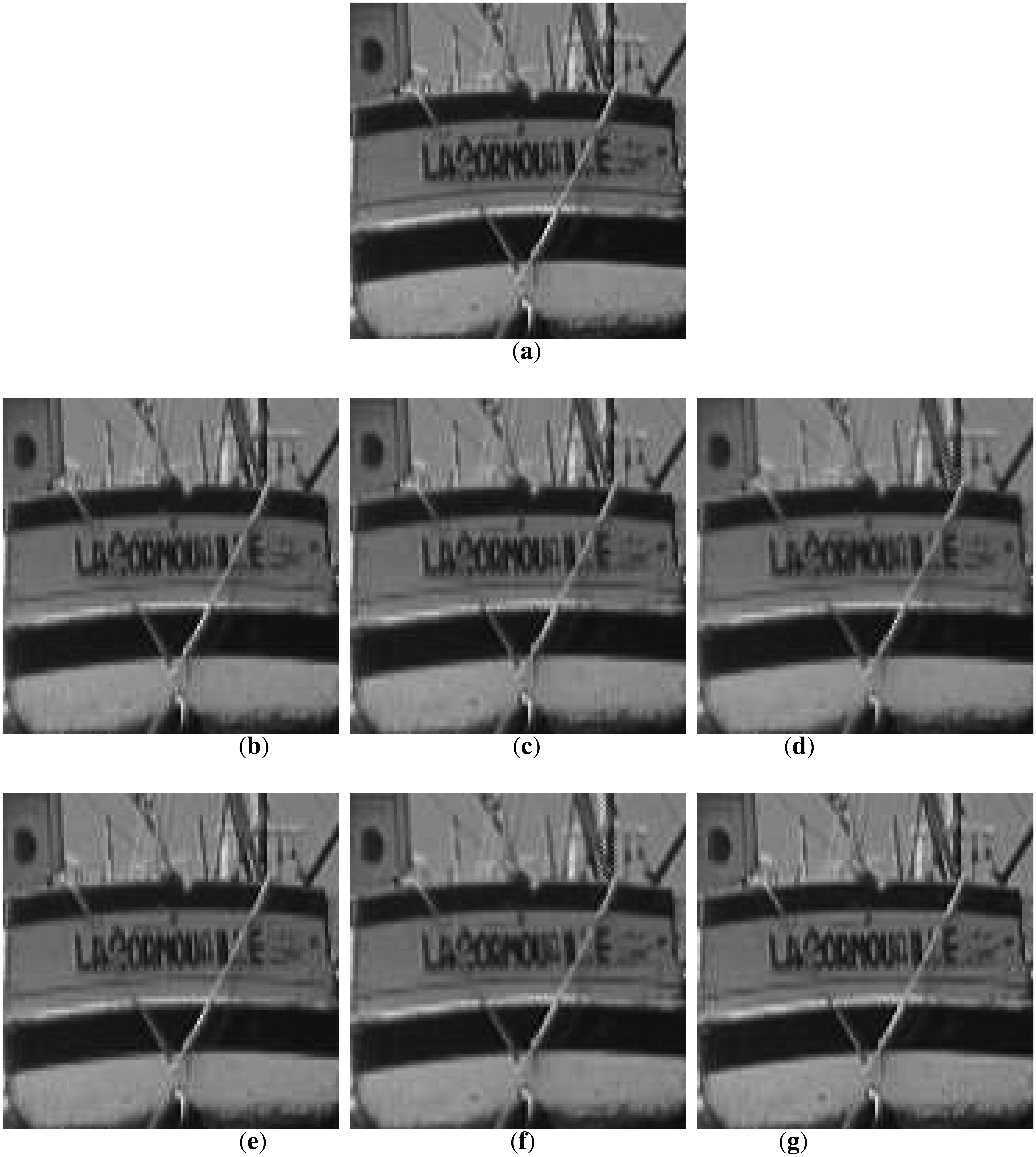
The Barbara image in Figure 4 has many low and high-angle directions that the previous methods may miss. Figure 4(a–g) shows poor performance because only a limited number of edge directions were utilized, which does not compensate for inaccurate edge information. Figure 4(h,i) shows better results than the other conventional methods. However, the diagonal edge reconstruction is not sufficient. The proposed method, however, performs well for this case as shown in Figure 4(j). Figure 5 shows the results for the Boat image. The result for this image also shows that the proposed method is superior to other methods.

4. Conclusions

This paper presented an effective spatial deinterlacing method, which is achieved by improving the edge preserving ability of the conventional edge-based line average method. This filter consists of three steps: pre-determined six-tap filter based pre-processing step, FM-based weight assignation step, and rank-ordered marginal filter step. The experimental results indicated that ROMF has achieved these two goals and has promising performance subjectively and objectively. Meanwhile, ROMF has merits of low complexity for real-time application.

References

- Jack, K. Video Demystified—A Handbook for the Digital Engineer, 4th ed; Elsevier: Oxford, UK, 2005. [Google Scholar]
- Bellars, E.B.; Haan, G.D. Deinterlacing: A Key Technology for Scan Rate Conversion; Elsevier: Oxford, UK, 2000. [Google Scholar]
- Wu, J.; Paul, A.; Xing, Y.; Fang, Y.; Jeong, J.; Jiao, L.; Shi, G. Morphological dilation image coding with context weights prediction. Signal Process. Image Commun. 2010, 25, 717–728. [Google Scholar]
- Wu, W.; Liu, Z. Learning-based super resolution using kernel partial least squares. Image Vis. Comput. 2011, 29, 394–406. [Google Scholar]
- Wu, J.; Huang, J.; Jeon, G.; Jeong, J.; Jiao, L.C. An adaptive autoregressive de-interlacing method. Opt. Eng. 2011, 50. [Google Scholar] [CrossRef]
- Wu, J.; Liu, Z.; Gueaieb, W.; He, X. Single-image super-resolution based on Markov random field and contourlet transform. J. Electron. Image 2011, 20. [Google Scholar] [CrossRef]
- Wu, J.; Li, T.; Hsieh, T.-J.; Chang, Y.-L.; Huang, B. Digital signal processor-based 3D wavelet error-resilient lossless compression of high-resolution spectrometer data. J. Appl. Remote Sens. 2011, 5. [Google Scholar] [CrossRef]
- Wu, J.; Liu, Z.; Krys, D. Improving laser image resolution for pitting corrosion measurement using markov random field method. Autom. Constr. 2012, 21, 172–183. [Google Scholar]
- Kim, W.; Jin, S.; Jeong, J. Novel intra deinterlacing algorithm using content adaptive interpolation. IEEE Trans. Cons. Electron. 2007, 53, 1036–1043. [Google Scholar]
- Lee, D.-H. A new edge-based intra-field interpolation method for deinterlacing using locally adaptive-thresholded binary image. IEEE Trans. Cons. Electton. 2008, 54, 110–115. [Google Scholar]
- Yang, S.; Kim, D.; Jeong, J. Fine edge-preserving deinterlacing algorithm for progressive display. IEEE Trans. Cons. Elect 2009, 55, 1654–1662. [Google Scholar]
- Park, S.J.; Jeon, G.; Jeong, J. Covariance-Based Adaptive Deinterlacing Method Using Edge Map. Proceedings of the IEEE IPTA2010, Paris, France, July 2010; pp. 166–171.
- Park, S.J.; Jeong, J. Local surface model-based deinterlacing algorithm. Opt. Eng. 2011, 50. [Google Scholar] [CrossRef]
- Jeon, G.; Anisetti, M.; Kim, D.; Bellandi, V.; Damiani, E.; Jeong, J. Fuzzy rough sets hybrid scheme for motion and scene complexity adaptive deinterlacing. Image Vis. Comput. 2009, 27, 425–436. [Google Scholar]
- George, A.; Romaguera, S. Characterizing completable fuzzy metric spaces. Fuzzy Set. Syst. 2004, 144, 411–420. [Google Scholar]
- Hong, S.M.; Park, S.-J.; Jeong, J. Deinterlacing algorithm using fixed directional interpolation filter and adaptive distance weighting scheme. SPIE Opt. Eng. 2011, 50. [Google Scholar] [CrossRef]