A Small and Slim Coaxial Probe for Single Rice Grain Moisture Sensing


Abstract
: A moisture detection of single rice grains using a slim and small open-ended coaxial probe is presented. The coaxial probe is suitable for the nondestructive measurement of moisture values in the rice grains ranging from from 9.5% to 26%. Empirical polynomial models are developed to predict the gravimetric moisture content of rice based on measured reflection coefficients using a vector network analyzer. The relationship between the reflection coefficient and relative permittivity were also created using a regression method and expressed in a polynomial model, whose model coefficients were obtained by fitting the data from Finite Element-based simulation. Besides, the designed single rice grain sample holder and experimental set-up were shown. The measurement of single rice grains in this study is more precise compared to the measurement in conventional bulk rice grains, as the random air gap present in the bulk rice grains is excluded.1. Introduction
Recently, there has been an increased interest in microwave measurement techniques for the determination of moisture content, m.c. (or dielectric properties) of bulk rice grains in the microwave frequencies range [1–5]. This is due to the fact that the moisture percentage (wet basis m.c., ranging from 9% to 26%) in the rice grains plays an important role in the rice marketing and storage aspects. In marketing, the price of rice is dependent on the weight of the bulk rice, so accumulation of water in the rice grain will increase the price of rice. On the other hand, the moisture content in the grain mass determines the storage duration of the rice grains, in which m.c. < 13% indicates a storage duration of more than 60 days [6,7].
The m.c. of rice grains can be determined by either direct [8] or indirect methods [1–7]. Direct methods determine the m.cd by removing the moisture of the grains using oven drying methods (heating at 130 °C) or chemical reaction methods (extracting water using the reaction of iodine in sulfur dioxide). Both methods remove the moisture determine the true water content by the resulting weight loss. Indirect methods, in contrast, require the measurement of an electrical property of the grain using an instrument, a grain moisture meter. For very low frequency (DC) measurements, the desired electrical parameters are conductance, capacitance and resistance of the rice gain. The absorption power, resonant frequency, attenuation constant, reflection constant and transmission constant of the rice grain are the measured parameters of interest in microwave frequency measurements. Changes in electrical properties (or microwave properties) that can be directly correlated with a change in actual m.c. of the rice grain are obtained from the oven drying method (direct method). Recently, indirect methods have become more popular than direct methods due to their rapid tests and user friendly features.
The prime considerations in the measurement of grain moisture using indirect methods are the size of the instrument sensor, which is in direct contact with the rice grain samples and the accuracy of the measurements [5]. Various microwave waveguide methods were proposed for the above purpose, but some of those methods require specify dimensions of the rice grain bulk to fit inside the given size of the waveguide [2–4]. However, the rice grain bulk is composed of a mixture of air and rice grains. The random distribution of rice grains and the air gap causes a low repeatability and low precision in the measurements. Among the mentioned methods, an open-ended waveguide method is the simplest and a nondestructive way to measure the m.c. of rice grains. The measurement using commercial open-ended waveguides is suitable for a specific rice grains size (width and length). This is because the waves scattered from the waveguide aperture would penetratd through small single rice grains as the small rice grains faed to entirely cover the aperture area of commercial probes.
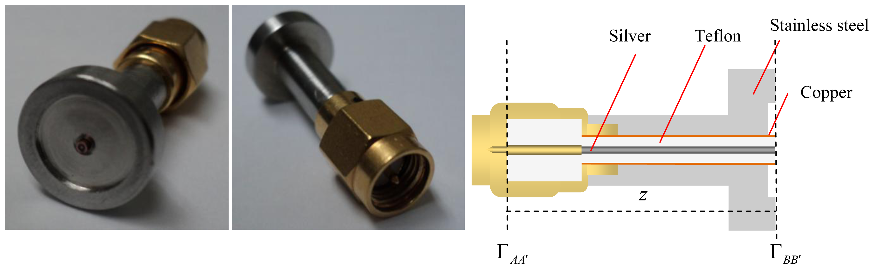
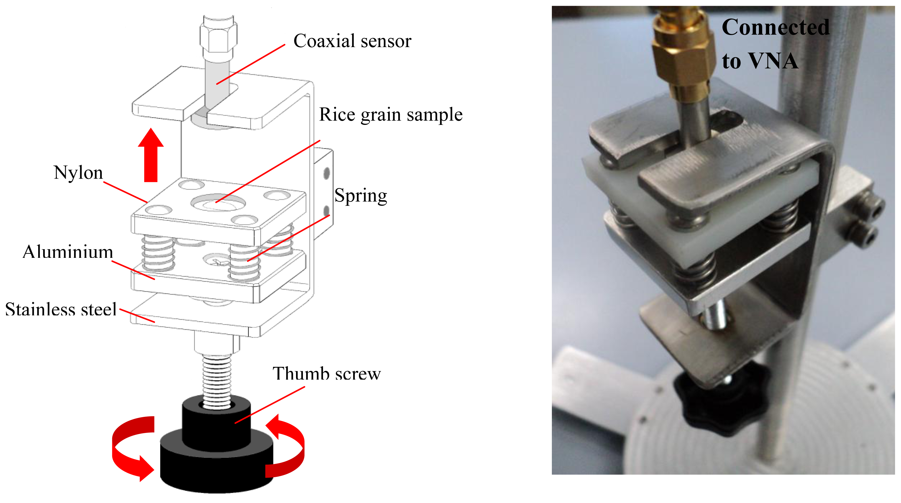
In this study, a millimeter size slim open-ended coaxial probe has been fabricated to measure the moisture in small grains. The coaxial probe was fabricated from a 0.86 mm outer diameter (OD) semi-rigid coaxial cable equipped with a male-type SMA plug connector. The coaxial cable was machined flat and polished to form an open surface end. Then, the coaxial probe was protected and covered by a customized stainless steel sheath with a flange, as shown in Figures 1 and 2. Here, the main focus is put on the aperture of the probe placed against a rice grain sample ranging from 9% m.c. to 26% m.c. Typically, the open-ended coaxial probe is calibrated by using open air, short terminator and liquid load. Directivity error, source match error, and frequency tracking are corrected by this technique. Besides that, the rapid and simple calibration of the coaxial sensor without the use of short and load calibration kits were also proposed in this study (discussed in Section 3.2).
2. Configuration and Dimensions Coaxial Sensor
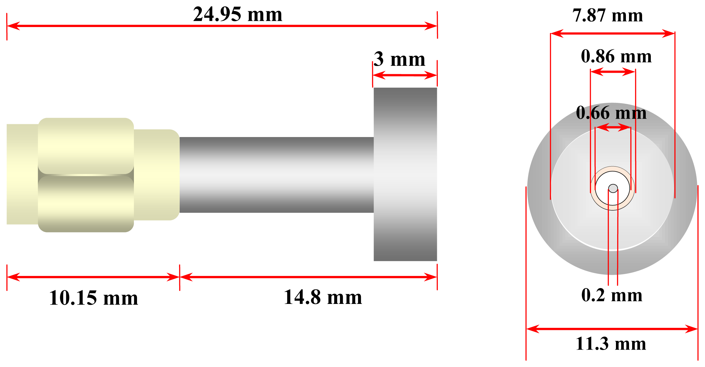
Figure 1 shows the side and the front sectional views of our milimeter size coaxial probe. The front sectional aperture of coaxial probe shows 2a = 0.20 mm diameter of inner conductor, 2b = 0.66 mm diameter of coaxial-filled Teflon and 0.86 mm diameter of the outer conductor. The coaxial-filled Teflon supports the coaxial line between the outer conductor and the inner conductor. Both inner and outer conductors guide the propagation wave in the coaxial line. In addition, an 11.3 mm total diameter steel flange is used to cover the total fringing field at the aperture probe. Figure 2 shows a picture and cross sectional structure of the coaxial probe.
3. Sensor Model
3.1. Reflection Coefficient Model
The reflection coefficient, Γ models of the millimeter coaxial probe are given as:
The complex parameters in Equation (1) was obtained by fitting the polynomial coefficients with calculated values obtained from the Finite Element Method using the COMCOL simulator over a broad range of permittivity values. The complex polynomial coefficients with seven decimals for Equation (1) are listed in Table 1. Equation (1) is valid for small coaxial probes, satisfying the relative permittivity, εr from 1 to 40 and the operation frequency from 0.4 GHz to 20 GHz. Comparison between the calculated and FEM simulated values for the reflection coefficient, Γ is shown in Table 2. If the FEM simulation results are used as the reference value, it is found that the percentage of relative error between both magnitudes of reflection coefficient will be less than 1%.
3.2. Calibration Model
In this study; the simplest technique of de-embedding of coaxial probe is by extending the transmission phase in which the phase of reflection coefficient at measurement plane; AA′ is extended towards the open end of coaxial probe; BB′ using exponential term of exp (j2kcz). First; a full one-port calibration technique was implemented at the AA′ plane using a commercial HP 85052D 3.5 mm calibration kit (open; short and load) which is only for network analyzer and cable error corrections. Secondly; under the assumption of quasi-TEM mode; the measured reflection coefficient; ΓAA′ of the sample at the plane AA′ can be de-embedded to the end of the probe connector which coincide with the calibration plane BB′ to give a reflection coefficient; ΓBB′ by [9]:
Simultaneously, the attenuation constant, α in the coaxial line can be found from the optimized length, z as:
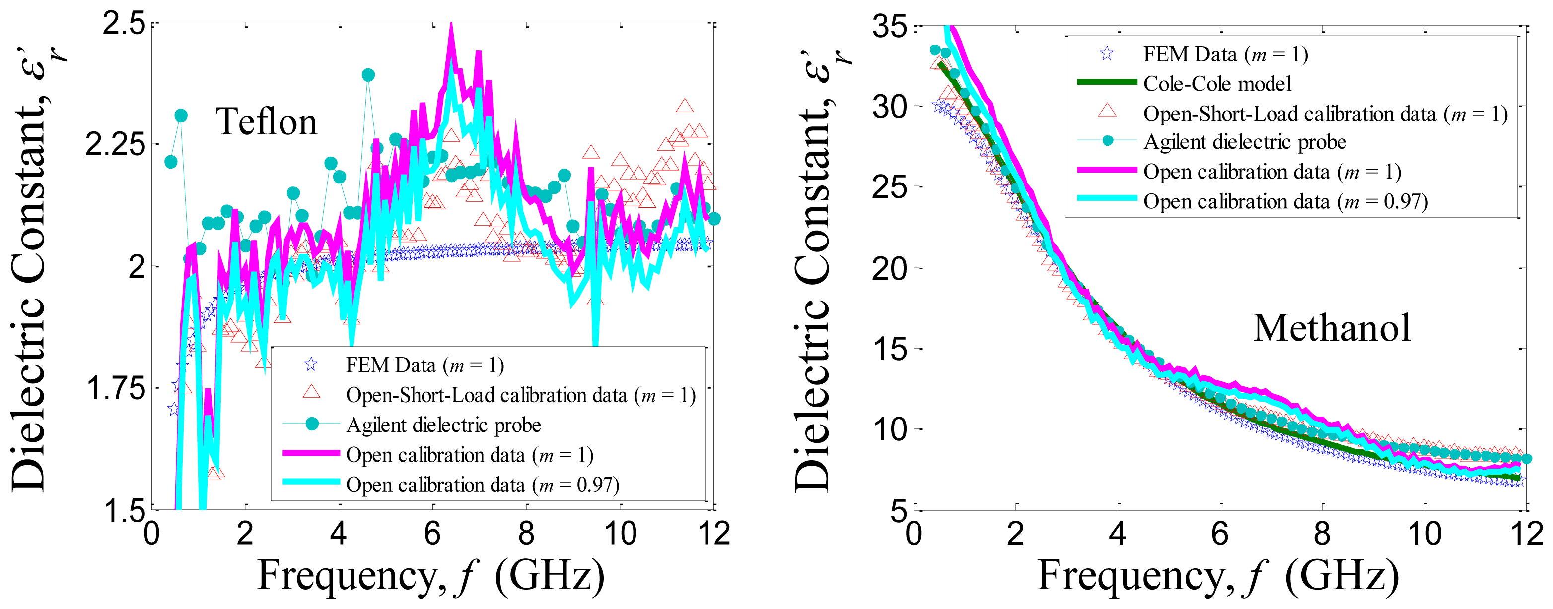
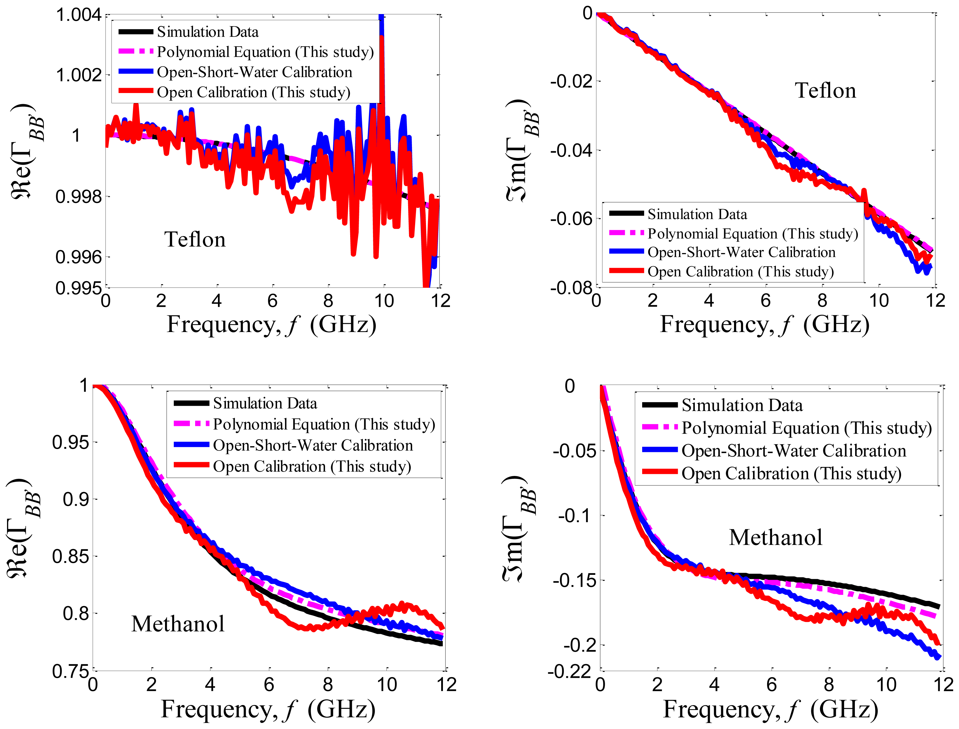
Teflon and methanol liquid have been tested to verify the accuracy of the proposed calibration method. Figure 3 shows the comparison between the calibrated reflection coefficient measurement and the simulation results. In simulation, the relative permittivity, εr of Teflon was 2.05. While, the relative permittivity, εr, of methanol was computed by Cole-Cole model with parameters: εs = 33.7, ε∞ = 4.45, τ = 4.95 × 10⁻¹¹ s and α = 0.036 [10]. The Cole-Cole model is:
In comparison, the calibrated measurement results using only the open standard have given a satisfy accuracy measurement up to 5 GHz. However, the noise inherent in both calibrated measurements are due to random errors contributed by the instruments or environmental measurement control. Moreover, the random errors are not taken into account in either calibration technique. The effect of the standing wave in the measurement of the open standard calibration becomes increasingly obvious when the operating frequency, f, is above 5 GHz.
The incident wave from the plane AA′ is transmitted to the plane BB′ by shifting phase of kcz, and is reflected back to input AA′ with the same shifting phase. Thus, the aperture reflection coefficient, ΓBB’ at the plane BB’ can be found by the phase delay of 2kcz with respect to the measured ΓAA’ at the plane AA′ and the transmission line relationship is given as in Equation (2). However, the transmission line is imperfect and a fringing field occurs near the aperture probe. Hence, a phase shift between the forward wave and the reflected wave occurs, and produces the standing wave due to the superposition between the incident wave and the reflected wave inside the coaxial line [11]. The standing wave effect can be ignored if the operation quarter wave length, λ/4 in the coaxial line is large than the physical length, z of coaxial line. For instance, 5 GHz of operation frequency will give λ/4 = 15 mm which is smaller than the physical length, z ≈ 22 mm, thus, the standing wave effect was significant when the operation frequency, f, was increased.
3.3. Inverse Model
For inverse solutions, the predicted values of the relative dielectric constant, εr,’ of a rice grain sample is obtained by minimizing the difference between the measured reflection coefficient, ΓBB’ and Equation (1), Γ by referring to the trial function, ψ:
Finding the zero routine was realized using the MATLAB fzero command. The initial approximate value in the numerical prediction was equal to 5 – j 0.001. The m terms in Equation (6) denote the weighted parameter for ratio of . The weighted parameter, m is suggested due to the measurement with calibration using Equation (2) (only open standard: εr = 1) does not consider the fringing effects for the medium loss samples. The predicted dielectric constant, for Teflon and methanol liquid over frequencies 0.5 GHz to 12 GHz at room temperature (25 °C) are validated and compared with the FEM simulation, Cole-Cole models and the Agilent 85070E dielectric probe as shown in Figure 4. The diameter of outer radius for the Agilent 85070E probe (2b = 3 mm) is approximately 4.5 times larger than the studied coaxial probe.
4. Experimental
The measurement reflection coefficient using millimeter coaxial probe that consists of the Agilent E5071C network analyzer in the frequency range between 0.5 GHz to 12 GHz was carried out at room temperature. The open end of the coaxial line was terminated by single rice grain sample. Normally, the length and width for various kinds of rice grains was in the range of 4.8–7.8 mm and 1.5–2.8 mm, respectively. Thus, the fringing field (sensing area ≈ 2b) [9] from the coaxial probe aperture was sufficiently covered by the single rice sample. This can be applied based on the principle that the different signals are reflected from the terminal surface of the moist grain through the coaxial opening.
Jati™ long grain white rice grown on the fertile soil of Kedah, the Rice Bowl of Malaysia, was used as the experimental sample. The rice grains were divided into different groups of 200 g per group. Each group of grains was sprayed with different estimated quantities of distilled water to achieve desired moisture levels. The bulk grains in each respective group were stirred and sealed in a container at 4 °C for 72 h to ensure a uniform water distribution within the bulk grains. The grains were conditioned to room temperature for 10 h prior to the measurements. Finally, 10 g of each group of bulk grain rice was dried in an air convection oven at 130 °C for 24 h [8]. The average moisture content, m.c. (in unit %) of each group of bulk rice grain was calculated on a wet basis as:
In this measurement, a specific holder was customized for the measurement of a selected single rice grain. The customized holder has a movable nylon platform which was mounted on a retort stand as shown in Figure 5. A single rice grain was randomly selected from each 10 g of bulk grain and placed into a narrow and depth concave surface at the center of the platform. The steel flange of the coaxial probe was rigidly entered from the holder edge into a narrow space interval. The rice grain on the nylon platform was moved forward to the aperture coaxial probe by using a thumb screw. The concave circular surface on platform was used as a probe guide to ensure that the probe aperture is exactly touching the rice sample. The four springs were employed to ensure that the aperture probe contacts firmly with the interface single rice grain and to avoid the errors in the measurement of interface air gaps.
5. Results and Discussion
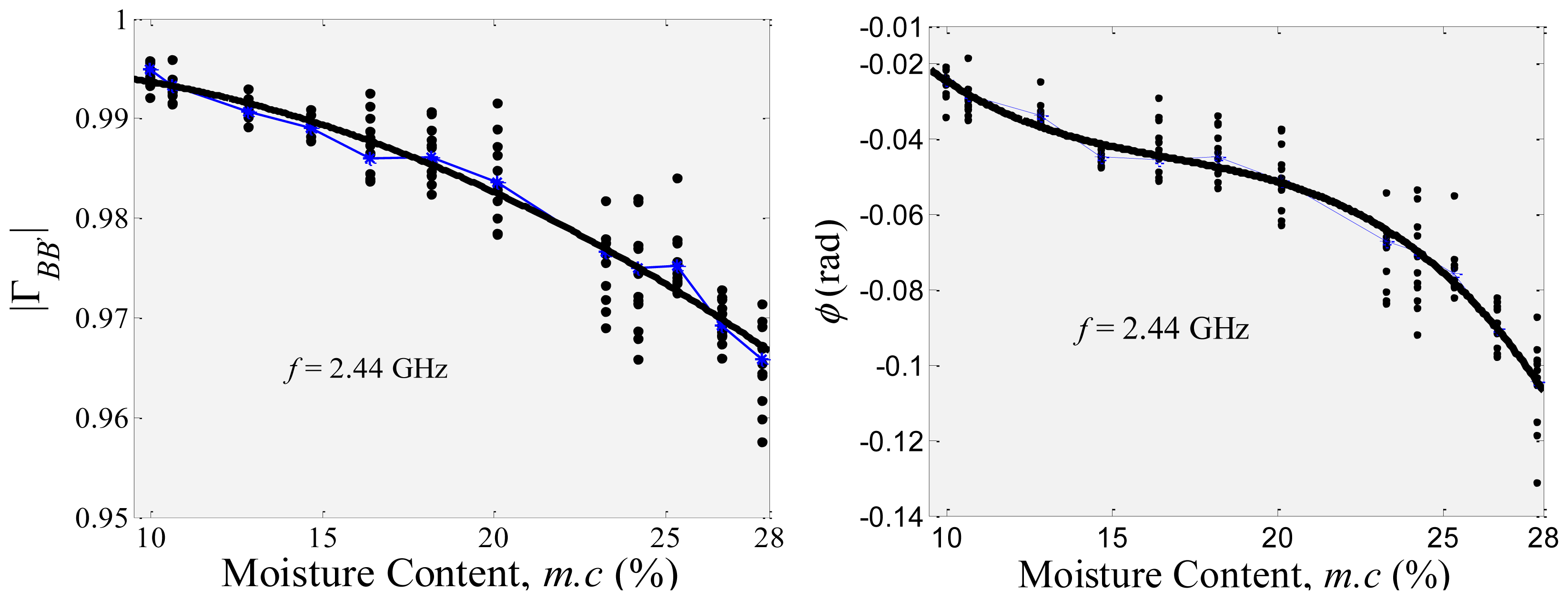
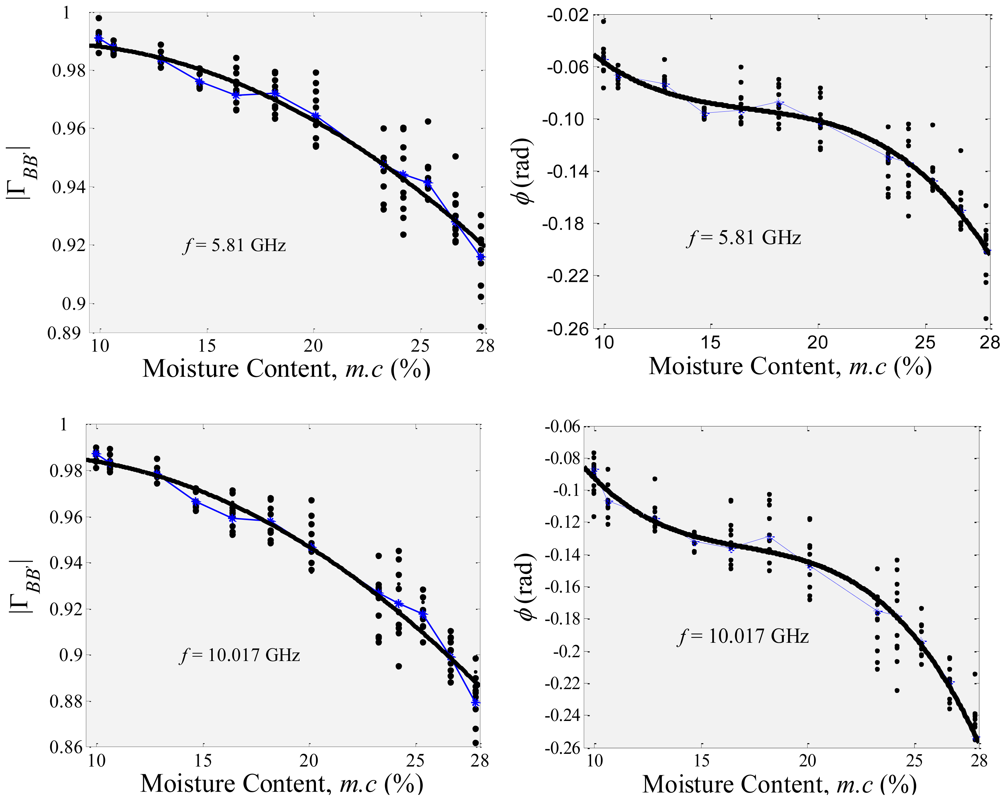
Figure 6 shows the reflection coefficient, ΓBB′, for 10 selected single rice grains from a bulk rice grain sample, where the bulk has a certain average water content, measured using the millimeter coaxial probe. As known, the m.c. for a bulk rice grain sample (which consists of thousands of single rice grains) is a statistical mean value due to the slightly different m.csingle of each single grain. Thus, the deviation of the actual m.csingle distribution in a single rice grain is higher as compared to the average m.c. of the entire bulk rice sample. This will lead to a scattered measurement of the reflection coefficient, ΓBB’, of the single grain in referring to the average m.c. of the bulk sample, as shown in Figure 6. However, Figure 6 does show a significant change of the measured reflection coefficient, ΓBB’ of a single rice grain with the m.c. of bulk rice grain. The black solid line in Figure 6 is a regression fitting line from the average of measured reflection coefficient data (blue point-line). The average of the measured reflection coefficients was obtained from the 10 data points of the measured reflection coefficients for each bulk moisture content, m.c. The rice moisture calculations are based on a gravimetric method, thus differential effects of density between the bulk rice and the single rice grain in the measurement were ignored. In this study, the 2.44 GHz and the 5.81 GHz frequencies were chosen due to the fact those frequencies correspond to a free unlicensed band which is specifically for industrial, scientific and medical (ISM) measurement purposes. The 10.02 GHz band was also chosen, since the dielectric loss for the water is greater at around 10 GHz and thus provides a comparative approach for the rice measurements at higher frequencies.
The polynomial regressions for the reflection coefficient, ΓBB’ (magnitude, |ΓBB’| and phase, ø) with respect to m.c. (in % units), are given in Equation (8) as listed in Table 3. Subsequently, Equation (8) was used by the coaxial probe to predict the m.c. (in % units), in a rice grain. It was found that, at higher frequencies, the point of measured reflection coefficient, ΓBB’ shows a large variation of m.c. (in % units) of rice grains.
The variations in relative dielectric constant,
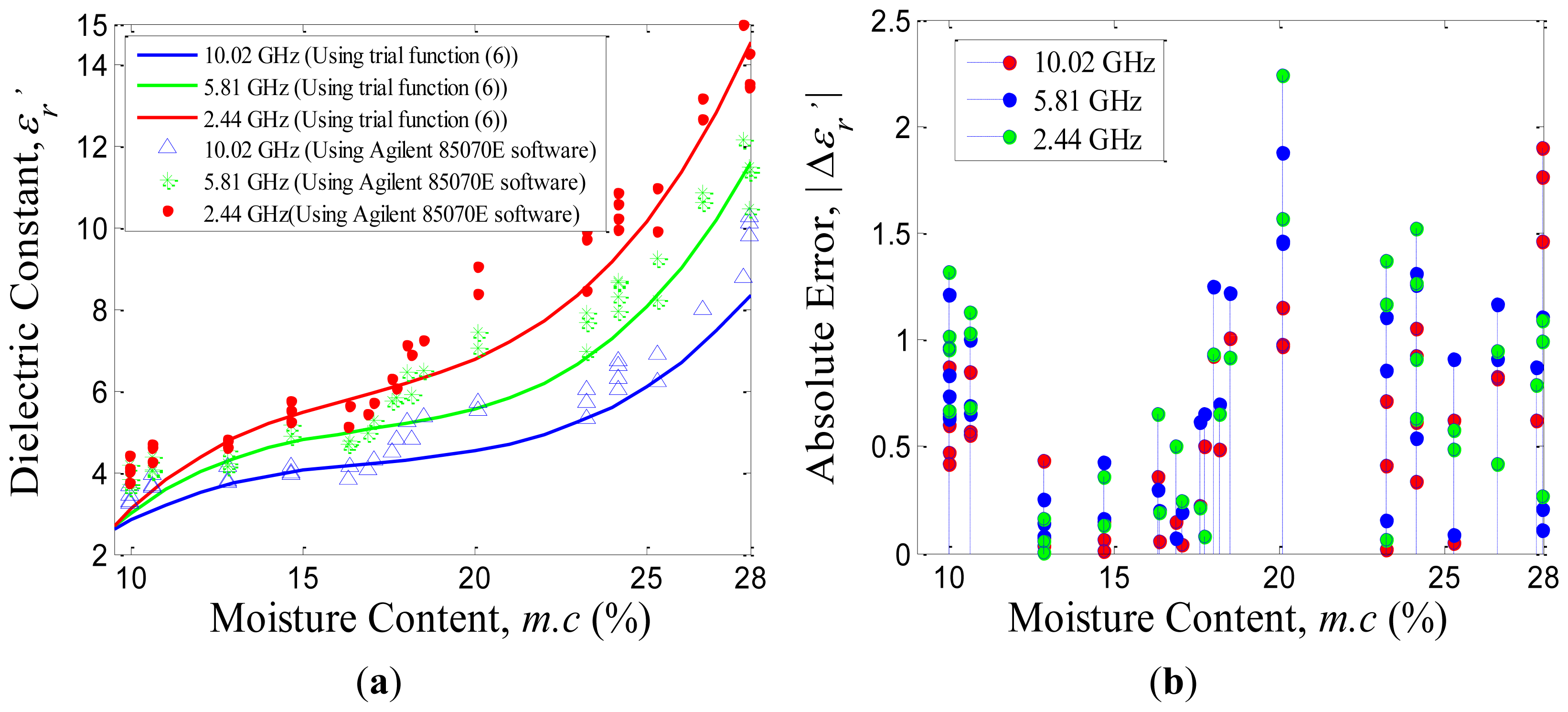
, of rice grains with the percentage of m.c. at 2.44 GHz, 5.81 GHz and 10.02 GHz, respectively, are plotted in Figure 7(a). The solid line of relative dielectric constant,
, in Figure 7(a) was the inverse of the reflection coefficient and refers to the trial function of Equation (6) with m = 1. The real part, ℜe(ΓBB’) and imaginary part,
 (ΓBB’) in Equation (6) were calculated by using relationship of ℜe(ΓBB’)+j (ΓBB’)=|ΓBB’|exp(jØ), where the values of |ΓBB’| and Ø were obtained from Equation (8), while, the reference values of ℜe(Γ) and
(Γ) in Equation (6) were computed using Equation (1). The measurement of dielectric constant points,
, of the single rice grain in Figure 7(a) were carried out using the studied coaxial probe with the Agilent 85070 E.06.01.36 software in order to verify the data obtained from the dielectric inversion work. The tolerance,
of dielectric constant prediction between both techniques is shown in Figure 7(b), which gives the maximum deviation,
≈ 2 for all frequencies ranging 9.5% m.c. to 28% m.c.
(ΓBB’) in Equation (6) were calculated by using relationship of ℜe(ΓBB’)+j (ΓBB’)=|ΓBB’|exp(jØ), where the values of |ΓBB’| and Ø were obtained from Equation (8), while, the reference values of ℜe(Γ) and
(Γ) in Equation (6) were computed using Equation (1). The measurement of dielectric constant points,
, of the single rice grain in Figure 7(a) were carried out using the studied coaxial probe with the Agilent 85070 E.06.01.36 software in order to verify the data obtained from the dielectric inversion work. The tolerance,
of dielectric constant prediction between both techniques is shown in Figure 7(b), which gives the maximum deviation,
≈ 2 for all frequencies ranging 9.5% m.c. to 28% m.c.
6. Conclusions
The proposed coaxial probe has a small sensing area which covers the size of single rice grain and provides a nondestructive and real time moisture measurement for single rice grains. Moreover, the single grain measurement does not depend on the bulk density of the rice grains, thus the uncertainty of bulk density in the rice measurement (due to different rates of broken rice in the bulk grain) can be ignored. In this study, moisture and dielectric models were created to suit the studied coaxial probe. The proposed simple de-embedding technique provides a rapid and low cost calibration procedure for the coaxial probe. However, the technique does not consider the systematic and random noises along the coaxial line, and thus it is suitable for a short coaxial probe, (z<λ/4) due to the significant standing wave that is produced inside the long coaxial line.
Acknowledgments
This study was supported by the Research University Grant (GUP) from Universiti Teknologi Malaysia under project number Q.J130000.2623.05J55.
References
- Yagihara, S.; Oyama, M.; Inoue, A.; Asano, M.; Sudo, S.; Shinyashiki, N. Dielectric relaxation measurement and analysis of restricted water structure in rice kernels. Meas. Sci. Technol. 2007, 18, 983–990. [Google Scholar]
- You, T.S.; Nelson, S.O. Microwave dielectric properties of rice kernels. J. Microw. Power Electromagn. Energy 1988, 23, 150–158. [Google Scholar]
- Jafari, F.; Khalid, K.; Yusoff, W.M.; Hassan, J. The analysis and design of multi-layer microstrip moisture sensor for rice grain. Biosyst. Eng. 2010, 106, 324–331. [Google Scholar]
- Kim, K.B.; Kim, J.H.; Lee, S.S.; Noh, S.H. Measurement of grain moisture content using microwave attenuation at 10.5 gHz and moisture density. IEEE Trans. Instrum. Meas. 2002, 51, 72–77. [Google Scholar]
- Nelson, S.O.; Kandala, C.V.K.; Lawrence, K.C. Moisture determination in single grain kernels and nuts by rf impedance measurements. IEEE Trans. Instrum. Meas. 1992, 41, 1027–1031. [Google Scholar]
- You, K.Y.; Salleh, J.; Abbas, Z.; You, L.L. Cylindrical Slot Antennas for Monitoring the Quality of Milled Rice. Proceedings of the PIERS, Suzhou, China, 12–16 September 2011; pp. 1370–1373.
- Thakur, S.K.P.; Kolmes, W.S. Permittivity of Rice Grain from Electromagnetic Scattering. Proceedings of the 4th International Conference on Electromagnetic Wave Interaction with Water and Moist Substance, Weimer, Germany, 13–16 May 2001; pp. 203–210.
- Moisture Measurements-Unground Grain and Seeds; ASABE Standards S352.1; ASABE: St. Joseph, MI, USA, 2000.
- You, K.Y.; Abbas, Z.; Khalid, K. Application of microwave moisture sensor for determination of oil palm fruit ripeness. Meas. Sci. Rev. 2010, 10, 7–14. [Google Scholar]
- Blackham, D.V.; Pollard, R.D. An improved technique for permittivity measurements using a coaxial probe. IEEE Trans. Instrum. Meas. 1997, 46, 1093–1099. [Google Scholar]
- You, K.Y.; Salleh, J.; Abbas, Z. Effects of length and diameter of open-ended coaxial sensor on its reflection coefficient. RadioEngineering 2012, 21, 496–503. [Google Scholar]


| Complex Coefficients in Equation (1) | |||||||
|---|---|---|---|---|---|---|---|
| δ0 | −1.2489993 × 10−42 −j2.8394016 × 10−42 | β0 | 4.068759 × 10⁻³² + j6.0446093 × 10−32 | γ0 | −2.3422556 × 10⁻²² − j1.0834847 × 10−21 | χ0 | 3.2710002 × 10⁻¹³ + j4.3278983 × 10−13 |
| δ 1 | 2.8571222 × 10−40 + j3.768492 × 10−40 | β1 | −8.0370086 × 10⁻³⁰ − j7.583469 × 10−30 | γ1 | 4.4984192 × 10⁻²⁰ + j1.5879853 × 10−19 | χ1 | −6.0520681 × 10⁻¹¹ − j5.0636272 × 10−11 |
| δ2 | −2.3273679 × 10−38 − j1.5437565 × 10−38 | β2 | 5.7873753 × 10⁻²⁸ + j2.8089148 × 10−28 | γ2 | −3.0910003 × 10⁻¹⁸ − j9.0522701 × 10−18 | χ2 | 4.0103924 × 10⁻⁹ + j1.6441936 × 10−9 |
| δ3 | 7.6388153 × 10−37 + j6.415406 × 10−38 | β3 | −1.6900591 × 10⁻²⁶ − j8.6931643 × 10−28 | γ3 | 8.3505821 × 10⁻¹⁷ + j2.6457801 × 10−16 | χ3 | −1.0502173 × 10⁻⁷ + j7.2034269 × 10−10 |
| δ4 | -6.5374999 × 10−36 + j5.4983527 × 10−36 | β4 | 1.7398403 × 10⁻²⁵ − j3.1661421 × 10−26 | γ4 | −7.5782519 × 10⁻¹⁶ − j5.0073506 × 10−15 | χ4 | 9.5824766 × 10⁻⁷ − j2.7560669 × 10−7 |
| δ5 | 2.124032 × 10⁻³⁵ − j1.2607055 × 10−35 | β5 | −4.0862657 × 10⁻²⁴ + j1.4318571 × 10−25 | γ5 | 3.2419268 × 10⁻¹⁵ + j6.0109573 × 10−14 | χ5 | −4.2081991 × 10⁻⁶ + j1.338741 × 10−6 |
| δ6 | −6.9741684 × 10⁻³⁵ − j9.6327922 × 10−36 | β6 | −2.122961 × 10⁻²⁵ − j4.29076 × 10−25 | γ6 | −8.983224 × 10⁻¹⁵ − j2.9066269 × 10−12 | χ6 | 1.1443542 × 10⁻⁵ − j3.7209467 × 10−6 |
| δ7 | 5.6295484 × 10⁻³⁵ − j1.6824543 × 10−35 | β7 | −1.1659675 × 10⁻²⁵ + j2.7664167 × 10−25 | γ7 | 7.1748551 × 10⁻¹⁵ − j7.8926933 × 10−14 | χ7 | 9.9999087 × 10⁻¹ + j2.5383631 × 10−6 |
| f (GHz) | Reflection Coefficient, Γ(εr= 1 – j 0) | Relative Error (%) | Reflection Coefficient, Γ(εr=40 – j 5) | Relative Error (%) | ||
|---|---|---|---|---|---|---|
| Equation (1) | Simulations | Equation (1) | Simulations | |||
| 1 | 0.9999955− j 0.002931223 | 0.9999957− j 0.002926868 | 0.00002 | 0.9855305− j 0.09609176 | 0.9824686− j 0.10045476 | 0.2646 |
| 10 | 0.9995828− j 0.02934018 | 0.9995701− j 0.02929747 | 0.00139 | 0.5257350− j 0.7289402 | 0.5155215− j 0.7370167 | 0.0745 |
| 18 | 0.9986448− j 0.05295265 | 0.9985924− j 0.05287694 | 0.00563 | 0.02905127− j 0.8579390 | 0.02131934− j 0.85924107 | 0.12505 |
| For f = 2.44 GHz, |ΓBB’| = −4.918756 × 10⁻⁵ m.c2 + 3.694446 × 10⁻⁴m.c + 0.9948964, Ø = −3.043213 × 10⁻⁵ m.c3 + 1.530463 × 10⁻³ m.c2 − 2.729901 × 10⁻²m.c + 0.1257916, |
| For f = 5.81 GHz, |ΓBB′| = −1.616480 × 10⁻⁴ m.c2 + 2.323330 × 10⁻³ m.c + 0.9810024, Ø = −6.330536 × 10⁻⁵m.c3 + 3.209160 × 10⁻³m.c2 − 5.643064 × 10⁻²m.c + 0.2498354, |
| For f = 10.07 GHz, |ΓBB′| = −2.135387 × 10⁻⁴ m.c2 + 2.691858 × 10⁻³ m.c + 0.9783604, Ø = −7.264877 × 10⁻⁵m.c3 + 3.722521 × 10⁻³m.c2 − 6.603589 × 10⁻²m.c + 0.2683548, |
•The symbol m.c refers to the percentage of bulk rice moisture content.
© 2013 by the authors; licensee MDPI, Basel, Switzerland. This article is an open access article distributed under the terms and conditions of the Creative Commons Attribution license (http://creativecommons.org/licenses/by/3.0/).
Share and Cite
You, K.Y.; Mun, H.K.; You, L.L.; Salleh, J.; Abbas, Z. A Small and Slim Coaxial Probe for Single Rice Grain Moisture Sensing. Sensors 2013, 13, 3652-3663. https://doi.org/10.3390/s130303652
You KY, Mun HK, You LL, Salleh J, Abbas Z. A Small and Slim Coaxial Probe for Single Rice Grain Moisture Sensing. Sensors. 2013; 13(3):3652-3663. https://doi.org/10.3390/s130303652
Chicago/Turabian StyleYou, Kok Yeow, Hou Kit Mun, Li Ling You, Jamaliah Salleh, and Zulkifly Abbas. 2013. "A Small and Slim Coaxial Probe for Single Rice Grain Moisture Sensing" Sensors 13, no. 3: 3652-3663. https://doi.org/10.3390/s130303652