New Approach Based on Compressive Sampling for Sample Rate Enhancement in DASs for Low-Cost Sensing Nodes


Abstract
: The paper deals with the problem of improving the maximum sample rate of analog-to-digital converters (ADCs) included in low cost wireless sensing nodes. To this aim, the authors propose an efficient acquisition strategy based on the combined use of high-resolution time-basis and compressive sampling. In particular, the high-resolution time-basis is adopted to provide a proper sequence of random sampling instants, and a suitable software procedure, based on compressive sampling approach, is exploited to reconstruct the signal of interest from the acquired samples. Thanks to the proposed strategy, the effective sample rate of the reconstructed signal can be as high as the frequency of the considered time-basis, thus significantly improving the inherent ADC sample rate. Several tests are carried out in simulated and real conditions to assess the performance of the proposed acquisition strategy in terms of reconstruction error. In particular, the results obtained in experimental tests with ADC included in actual 8- and 32-bits microcontrollers highlight the possibility of achieving effective sample rate up to 50 times higher than that of the original ADC sample rate.1. Introduction
In recent years, embedded systems (such as microcontrollers, field programmable gated arrays, digital signal processors and so on) have been playing a fundamental role in metrological applications. The availability of integrated systems capable of digitizing, processing and transmitting measurement results offers the opportunity of realizing nodes for distributed and/or portable measurement systems characterized by reduced costs and good performance. Typical application examples are smart meters for energy billing or analysis of electrical power quality [1–4], monitoring of environmental quantities of interest [5–8], control of complex production process [9–11].
Architectures based on successive approximation registers are usually chosen for the Data Acquisition Section (DAS), mainly based on the Analog to Digital Converter (ADC) embedded in the measurements nodes, due to their straightforward implementation and a nominal vertical resolution that is suitable for most of the considered application. Nevertheless, some specific solutions for band-pass signals [12–14] and some dedicated solutions exploiting more performing ADCs (ΣΔ or flash converters) are also available on the market [15].
The most significant parameters commonly used for characterizing and determining the performance of the DAS are:
Nominal vertical resolution: usually expressed in bits, it defines how many distinct output codes the DAS can produce; depending on the specific architecture of the ADC, typical resolution varies between 10 and 14 bits;
Maximum sample rate: it defines the capability of the DAS of rapidly sampling and converting the input signal and directly determines the maximum spectral component that can be alias‐free sampled. Typical actual values for low cost microcontrollers range from few tens of kilohertz up to five MHz;
Memory depth: combined with the sample rate, it determines the maximum observation interval the microcontroller can acquire for successive processing. Values from few kilobytes up to some megabytes are usually found;
Input bandwidth: determines the maximum frequency of spectral components that the ADC can receive as input without significant distortion; to assure alias-free digitization of the input signal, it is usually set no higher than half maximum sample rate, even though some solutions dedicated to digital down conversion provide larger bandwidth [16].
For distributed measurement systems consisting of distributed acquisition nodes and a central computing unit that processes measurement data, improving the performance of the embedded DAS, in terms of sample rate enhancement, can be crucial for the improvement of the whole measurement system. To this aim, the paper presents a novel acquisition strategy, based on compressive sampling (CS), which permits to increase the maximum sample rate of DAS integrated in low‐cost microcontrollers.
CS is a recent and attractive sampling approach capable of assuring reliable reconstruction of signals of interest from a very reduced number of acquired samples, provided that some conditions about the signal and sampling scheme are met [17]. Some papers recently focused their attention on the possibility of exploiting CS to enhance the performance of ADC in terms of sample rate. In particular, in [18] CS is used to extend the traditional equivalent time sampling (ETS) scheme in order to reconstruct the input signal with a higher time resolution. However, a number of periods of the input signal much higher than those successively reconstructed are involved, which poses severe constraints on the stability of the time-base. Such problem has been solved for random sampling CS-based ADC in [19] through an ad-hoc new circuit. An alternative is represented by CS-based ADCs exploiting random demodulation [20], which have been shown to have good performance for most measurement applications [21].In particular, a significant improvement in terms of sample rate has been obtained, though at the expense of architectural complexity, due to the presence of the analog mixing of the input signal with a pseudo-random sequence.
Differently from the above-mentioned solutions, the method proposed hereinafter does not require any hardware modification (such as external clock circuits and/or analog mixing stages) to increase the sample rate and turns out to be the optimal solution for the majority of already available ADCs integrated in embedded systems. The proposed acquisition strategy permits, in fact, to achieve a higher time resolution when digitizing a signal included in the ADC bandwidth in real-time, by combining the already available hardware section (constituted by the traditional ADC and the high-resolution time-basis) with a proper software procedure, which provides a suitable random sequence of sampling instants and reconstructs the signal of interest according to the CS theory.
2. Problem Statement
Taking advantage of some attractive features of the CS theory, a new method is proposed in the following section with the aim of improving the nominal sample rate of ADCs. Although the proposed method is general, it proves particularly advantageous when applied to ADC modules included in low cost microcontrollers (MCs). The availability of a high-resolution time‐basis (such as that generated from the fundamental clock frequency for MCs) allows, in fact, finely defining a suitable random sequence of the sampling instants capable of assuring the reliable successive signal reconstruction. For the sake of clarity, the key idea underlying the method is described and compared both to the traditional and compressive sampling approach.
2.1. Traditional Sampling Approach
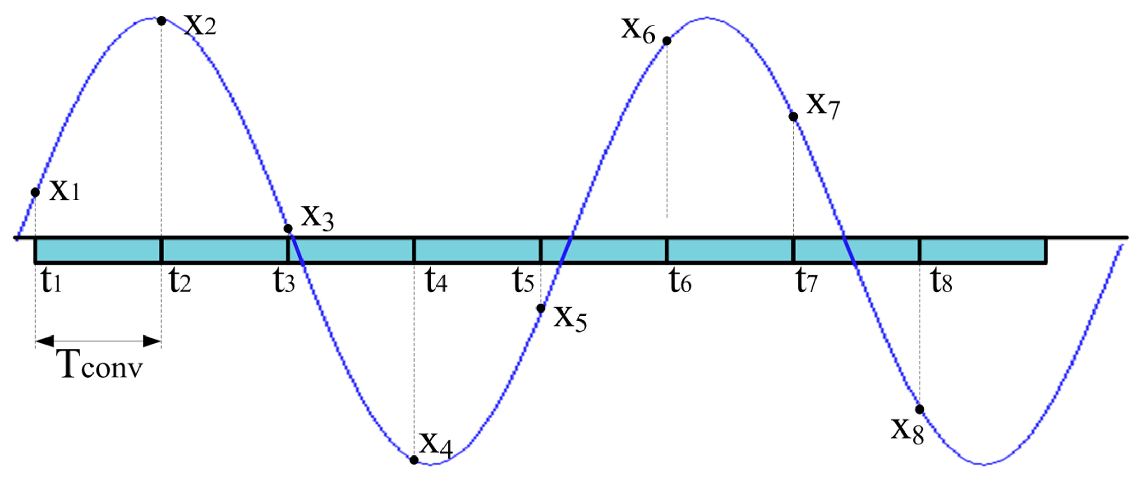
In Figure 1 the traditional sampling approach, adopted by the majority of ADCs, is shown. The ADC operates at its highest sampling rate and input signal samples are uniformly taken with a sampling period equal to Tconv, which is the time interval required by the ADC to digitize (i.e.,to sample and convert) a single sample. Alias-free sampling can be assured on a signal whose maximum spectral content is lower than 1/(2Tconv). It is useful to highlight that in the case of low-cost microcontrollers, the limited memory depth (usually shorter than 10,000 samples) permits to save only short-time records of the input signal.
2.2. CS-Based Sampling Approach
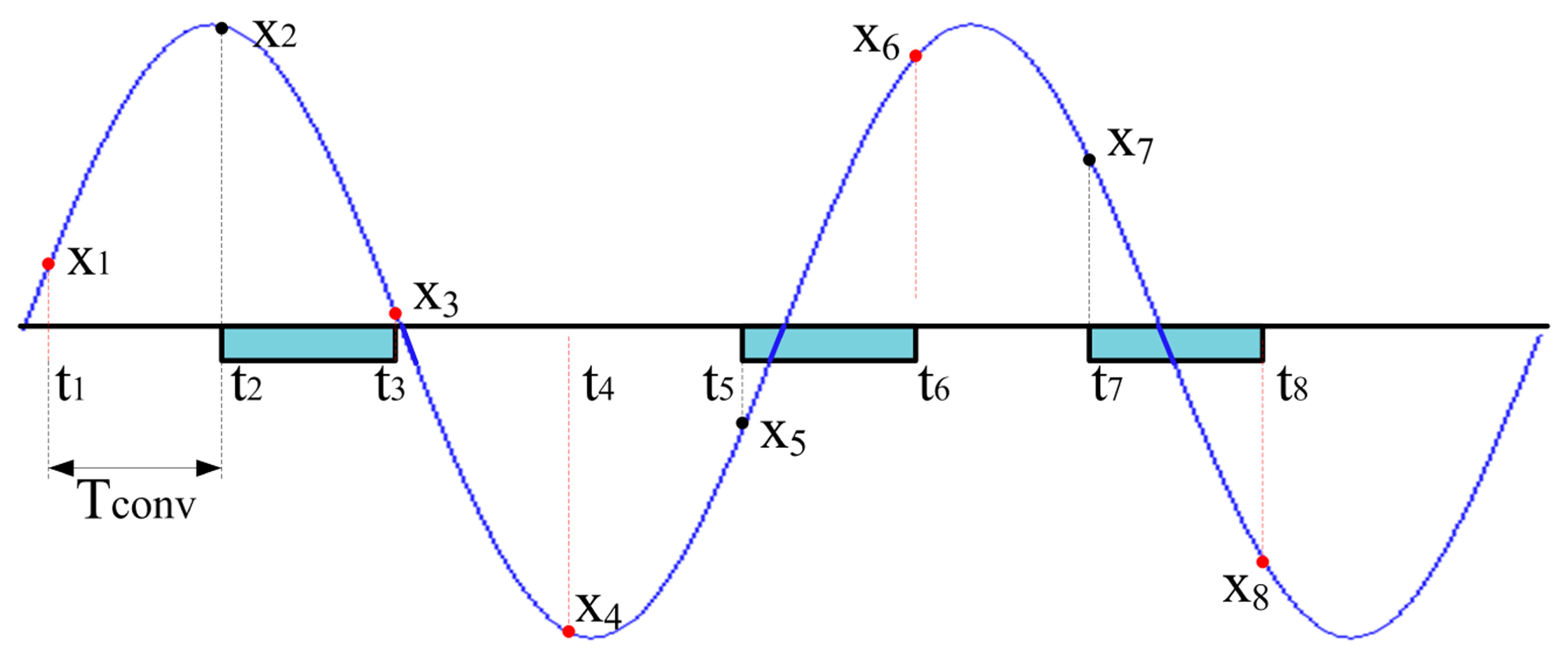
The authors recently faced the considered problem thanks to a suitable sampling approach based on CS [22–24]. As shown in Figure 2, if the samples (indicated by black dots) are randomly acquired throughout the observation interval, the signal of interest can accurately be reconstructed (samples marked by red dots) as it had been continuously digitized with a sampling period equal to Tconv.
It is worth noting that the desired reconstruction is achieved, starting from a very limited number of random signal samples. It was shown that accurate reconstruction can be gained, with a compression ratio up to 98% for multicomponent signals (i.e., 10,000 samples input signals were recovered starting from 200 acquired random samples).
2.3. Proposed Sample Rate Improvement
A new method (in the following referred to as new acquisition strategy) based on CS has been defined and implemented for increasing the effective sample rate of embedded DAS. The availability of a suitable time-basis allows finely setting the random sampling instants (i.e., the time instants the ADC starts to convert a single sample, which are marked as black dots in Figure 3), with a time resolution equal to Tc. Even though the conversion of a single sample takes a time Tconv greater than Tc (Tconv = 5Tc in the example shown in Figure 3), the proposed approach assures that the input signal will finally be reconstructed (red dots) at an effective sample rate equal to 1/Tc. As it can be expected, the only constraint is that the time difference between two successive actual sampling instants should be greater than Tconv.
3. Proposed Sampling Approach
To improve the sample rate of ADC in low‐cost embedded systems, the traditional hardware for analog-to-digital conversion has been complemented with a proper digital signal processing mandated to generate the random sequence of sampling instants and reconstruct the signal of interest from the acquired samples (Figure 4). In particular, the sequence of the random sampling instants is determined as a multiple of a high-resolution time-basis, Tc, and exploited to control the start of conversion (SOC) signal of the ADC. The sequence of considered instants and the corresponding samples (digitized at lower rate, equal to 1/Tconv, by the ADC) are given as input to the CS-based algorithm for the successive signal reconstruction, with a time resolution equal to that of the adopted time-basis. Specific details about the determination of the random sampling instants along with some guidelines for the reconstruction algorithm are given in the following.
3.1. Sampling Instants Determination
The first step of the new acquisition strategy is the determination of the actual sampling instants. According to the random sampling approach [25], the sampling instants ti are randomly chosen throughout the considered observation interval Tw equal to n times Tc. The key idea underlying the proposed sampling strategy is that the considered instants can be expressed as an integer multiple of the high-resolution time-basis Tc:
This way, the final signal reconstruction will be obtained with the same time resolution, thus granting a suitable enhancement of the nominal ADC sample rate. In order to assure proper operations of the CS-based ADC, the sampling instants ti have to satisfy the following expression (Figure 3)
Evaluation of a suitable acceptance threshold tsh, equal to m/n (only m sampling instants among n possible values have to be determined) in the first iteration;
Current sampling instant index ki is initially equal to 0;
A pseudo‐random number is generated according to uniform random distribution within the interval from 0 up to 1;
If the obtained pseudo‐random number is lower than the acceptance threshold, then ki is retained in sampling sequence and its value is updated by adding fr;
If the obtained pseudo‐random number is greater than the acceptance threshold, then ki is dropped and its value is incremented by one;
If the number of sampling instants included in the sequence is lower than m and ki is lower than n−1 return to step 3;
If ki is not lower than n but the sampling instants sequence is not yet full, a new acceptance threshold has to be calculated; this is particularly likely when the value mfr is close to n. To assure a fast convergence of the procedure, the authors adopted a threshold increment of 20%, i.e., the new value of tsh is 1.2 times the old tsh value; once updated the tsh value, return to step 2;
If the number of sampling instants included in the sequence is equal to m and ki value is lower than n−1, the sampling instants sequence is complete and can be adopted to acquire the samples of the input signal.
With regard to Tconv, since it is generated from the same fundamental clock, it usually is a multiple of the adopted time-basis; if this is not the case, the first multiple of Tc immediately greater than Tconv is used, thus granting that condition (2) always holds.
According to the CS approach [26], the relation between the sequence of acquired samples y ∈ ℝm and the input signal of interest x ∈ ℝn can be expressed as
3.2. Sensing Matrix Determination
Being usually m ≪ n (i.e., the number of equations lower than that of the unknowns), the problem of recovering x from the acquired samples through the equations system (3) results ill-posed [27] and cannot be solved via traditional approaches based on least squares minimization. The problem can, fortunately, be bypassed if a similar system can be written in the form
With reference to the measurement applications considered in Section I, most of the desired signals are characterized by sparse representations in the frequency domain. This way, the Fourier basis has been chosen and the corresponding matrix Ψ, whose entries are defined as
Thanks to the specific choice of the sampling matrix, the matrix A can be generated as a submatrix of ψ, thus reducing the computational burden of the method, since A doesn't have to be calculated from actual multiplications. It is, in fact, evaluated as the rows of the matrix ψ, whose indexes match those the sampling instants ki, thus granting its possible implementation also on devices characterized by reduced memory depth. With reference to the sampling matrix in Equation (4), the corresponding sensing matrix is given by:
3.3. Sparse Solution Evaluation
Even though the equations system in Equation (5) is still underdetermined, the sparsity of f can be exploited to find a suitable solution [28,29]. More specifically, it is possible to recover x by solving the following optimization problem
 (y) is a proper constraint that assures the consistence with the samples y. In particular, in the presence of noise-free samples, the feasible set
(y) can be expressed as
(y) is a proper constraint that assures the consistence with the samples y. In particular, in the presence of noise-free samples, the feasible set
(y) can be expressed as
If the acquired samples have been contaminated with small amount of noise ε (such as the quantization noise) a better expression would be
In other words, the best estimate f̂ of the input signal spectrum turns out to be the sparse representation characterized by the minimum l1-norm. The use of l1-norm grants, in fact, that obtained solution will be sparse, a condition that is usually not met when least square minimization approaches are adopted. Moreover, the constraints (11) and (12) define the so-called feasible set and assure that the required estimate f̂ is a solution (either absolute or approximated) of the Equation (5).
3.4. Input Signal Recovering
Once the solution f̂ is obtained, the input signal of interest can easily be recovered by means of Equation (6)
It is worth reminding that the time support of the recovered signal is the whole observation interval Tw and its quantization is related to the resolution of the time-basis adopted to define the sampling instants.
Finally, some considerations have to be drawn about the number of random digitized samples. In particular, it has been demonstrated [30] that the number of samples m has to meet the following condition:
The coherence proves to be a fundamental parameter for the compression in determining the number of needed samples. The lower its value, the fewer the samples required for a reliable reconstruction of f and consequently of the original signal x. According to the choices made about Φ and Ψ, the coherence reaches the minimum allowed value, equal to 1, in the considered acquisition strategy, thus granting a proper reconstruction of an S‐components signal with about S log n random samples. On the contrary, as it can be expected, the higher the number m of acquired samples, the lower the reconstruction error. However, as described in the following section, once the sparsity of the input signal is known, acquiring a larger number of samples proves to be not advantageous, since no more improvement in the reconstruction is experienced, while increasing the computational burden worthlessly.
4. Numerical Results
To preliminarily assess the performance of the proposed sampling strategy, several tests have been executed by means of numerical simulations. The effect of the most influencing parameters, such as number of acquired samples m, ADC sample rate fconv, ADC vertical resolution nbit, signal-to-noise ratio SNR, jitter and input signal sparsity S, has been evaluated. Parameters value has been chosen as close as possible to those provided by the cheapest microcontrollers [31] or granted by most of the embedded systems [32] that are currently available on the market. Similar values will be selected in the successive actual experimental tests. With regard to the number of acquired samples m, it has always been lower than typically available memory depth. On the contrary, the number of samples n granted for the signal reconstruction has been even much greater than memory depth, thanks to the CS-based approach.
As an example, some of the obtained results are presented in the following. Unless otherwise indicated, the input signal for tests has been a pure unipolar sinusoidal signal whose full scale amplitude and frequency were equal respectively to 2nbit−1 codes and 5 kHz; 80 random samples have been digitized with an effective vertical resolution of 12 bits at an ADC sample rate fconv equal to 10 kS/s, and the signal has been reconstructed over a time sequence of 10,000 samples at an effective sample rate fc of 1MS/s. For the sake of clarity, the parameters values are summarized in Table 1.
The reconstruction error has been used to assess the performance of the acquisition strategy. According to what stated in [13], it is defined as:
4.1. ADC Sample Rate and Vertical Resolution
A first set of tests aimed at verifying the dependence of the performance of the proposed acquisition strategy on the ADC conversion period and effective number of bits. Several nominal values of ADC sample rate fconv and vertical resolution nbit have been taken into account.
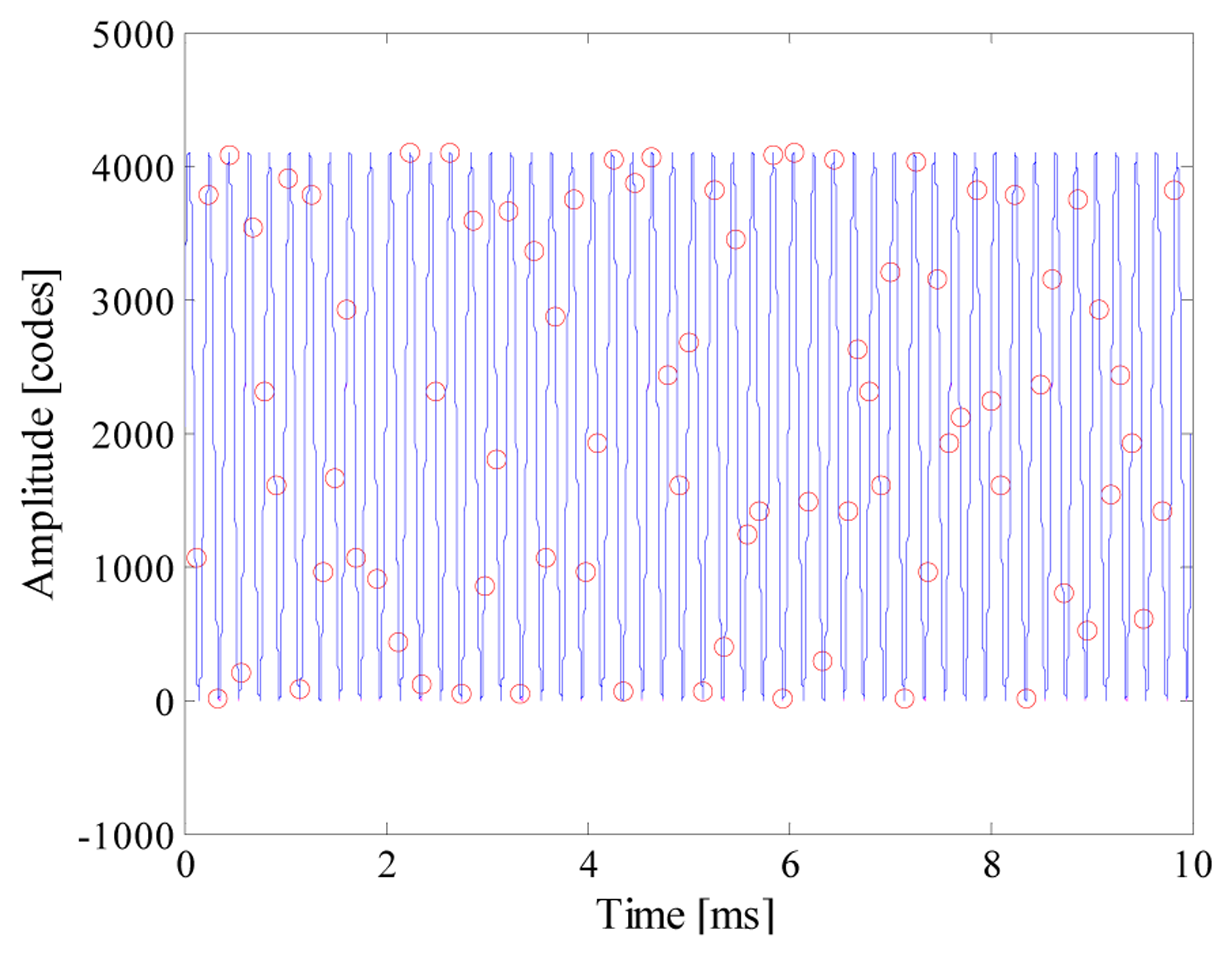
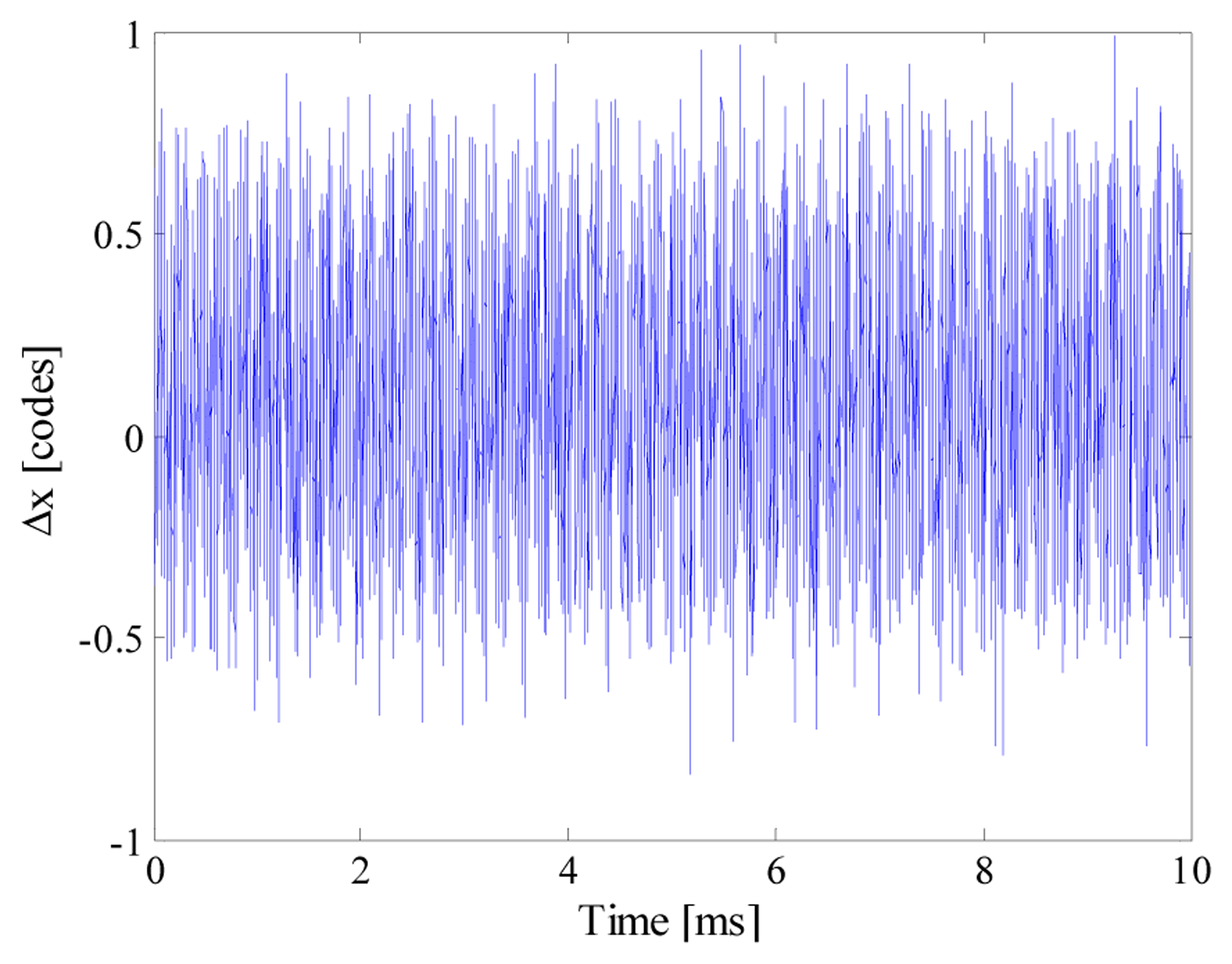
As an example, Figure 5 shows the input signal, the acquired samples and the reconstructed signal (which completely overlies the input signal) when nbit and fconv were equal respectively to 12 and 10 kS/s. It is worth noting that 80 samples are randomly taken throughout 50 periods of the input signal; the acquired sequence clearly violates the Nyquist theorem. To better appreciate the performance of the proposed acquisition strategy, point‐by‐point differences Δx between the reconstructed signal x̂ and the input signal x is shown in Figure 6. Differences greater than 1 code have never been found, thus assuring a reconstruction error as low as 0.007%.
Some results of the executed tests are summarized in Figure 7. As it can be seen, the performance of the acquisition strategy turned out to be almost independent from the nominal ADC sample rate. This way, the desired acquisition can be carried out by exploiting the ADC with the lowest available sample rate. It is so possible to make the ADC working in less critical conditions, thus allowing to take advantage of most of its effective number of bits.
Moreover, for each test configuration in terms of nbit and fconv, reconstruction error proved to be lower than the associated least significant bit (LSB), thus assuring that no harmful artifacts have been introduced by the proposed strategy. Finally, to compare the performance of the proposed acquisition strategy with that granted by the traditional CS approach [20], the same test has been executed with a tconv equal to tc for each value of nbit. The obtained values (i.e., the markers corresponding to a nominal ADC sample rate of 1 MHz in Figure 7) highlighted that no significant difference can be appreciated whatever the vertical resolution of ADC; this behavior can be easily explained if the equations system (5) is taken into account. Even though the authors have defined a suitable procedure for the generation of the random sequence of sampling instants, this choice involves no significant differences in solving the system (5). In other words, any random sequence is as good as any other from a theoretical point of view; only a negligible degradation in the mean performance is experienced, due to the time difference constraint (2) that slightly reduce the possible randomness of the sequence indexes. Similar considerations hold also in the other investigated test conditions.
4.2. Noise
The influence of the noise on the performance has successively been investigated. For each value of SNR, 1000 pseudo‐random sequences generated according to an additive white Gaussian noise (AWGN) have been added to the input signal; the average value of reconstruction errors have been evaluated. As an example, some results, obtained for different values of effective number of bits, are shown in Figure 8. As expected, the higher the SNR, the better the performance of the proposed acquisition strategy. In particular, reconstruction errors similar to those given in Figure 7 have been achieved only for the higher values of SNR.
4.3. Number of Acquired Samples and Effective Sample Rate
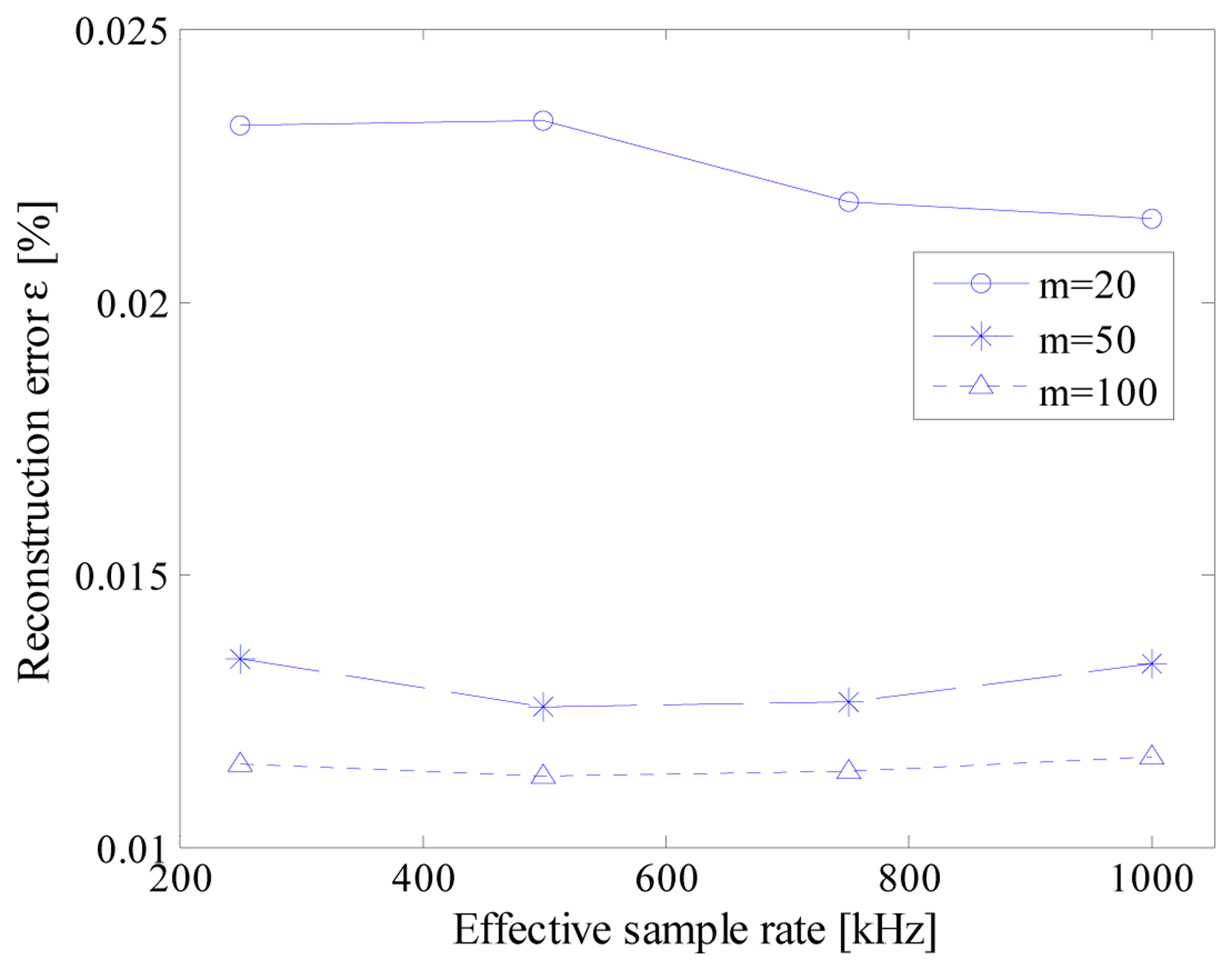
A number tests have then been performed for different combinations both of number of random samples m and effective sampling frequency fc. As an example, some results are summarized in Figure 9. As it can be appreciated, the difference between reconstructed and original signal is always lower than 1LSB, including when only 20 random samples are acquired, i.e., in the presence of a compression ratio equal to 99.8%.
4.4. Jitter
As stated above, all the clock signals (included the high-resolution time-basis adopted by the proposed acquisition strategy) of an embedded system are derived from a fundamental clock, usually referred to as instruction cycle clock, fCk. Due to the specific architecture of the microcontroller and the software implementation of the time-basis, a random difference between the nominal sampling instant and the effective one can occur. Such difference can be expressed in terms of number instruction cycles and typically assume integer values within 0 and 10 [32]. In other words, from the nominal SOC instant to its actual execution, a random number of instruction cycles could occur, due to latency or uninterruptable instructions problems. It is worth noting that this drawback can be mitigated, but not completely eliminated, and acts as a jitter on the high-resolution time-basis. Moreover, the actual jitter of the fundamental clock can be neglected in the following analysis, since its value is much lower than that associated with the instruction cycles. For the sake of the clarity, Figure 10a,b shows the actual SOC events (point-dashed lines) associated with a difference of two instruction cycles (TJt) from the nominal SOC event (dashed line) in the presence of ratios fCk/fc equal respectively to 1 and 4; the effect of the jitter on the actual digitized sample (circle marker) on the input signal (full line curve) is clearly reduced.
To analyze the effect of jitter, several scenarios have been simulated in terms of different values of ratio between instruction cycle clock frequency and effective sample rate. As an example, obtained results are presented in Figures 11 and 12 for jitter values of 10 (worst case) and 2 (reduced jitter) instruction cycles, respectively.
As it can be appreciated in Figure 11, 10 instruction cycles jitter highly degrades the performance of the proposed acquisition strategy. As expected, the worst results have been experienced when the effective sample rate matched the instruction cycle clock frequency; in this case, a difference with respect to the nominal value up to ten sampling instants can occur. Better results have been obtained for higher values of the ratio fCk/fc. However, values of reconstruction error never lower than 0.1% has been encountered. The performance of the proposed acquisition strategy improves if the jitter is reduced down to 2 instruction cycles (Figure 12). Reconstruction errors of few hundredths can, in fact, be assured with a suitable level of ratio fCk/fc.
4.5. Input Signal Sparsity
Finally, the reconstruction error has been evaluated versus different values of number of acquired samples and number of spectral components included in the input signal (i.e., the signal sparsity in frequency domain). Specific test parameters are presented in Table 2. As for the sparsity, its maximum value has been chosen according to Equation (14), once defined the highest number of random acquired samples. For each value of the signal sparsity 1000 numerical input signals have been generated by adding S spectral components whose amplitude, phase and location within the Nyquist band have been randomly selected. For each test configuration, minimum, average and maximum values of the reconstruction errors have been calculated in terms of m and S; some of the results are reported in Table 3.
As it can be expected, the higher the spectral content of the input signal, the higher the number of samples that have to be acquired in order to accurately reconstruct the signal. However, values of reconstruction error up to 10% has been experienced also when the input signal has been recovered from 100 random samples; this is mainly due to the effect of the considered jitter on spectral components characterized by higher frequency. This way, either the use of instruction cycle clocks with higher values of frequency or a greater number of random acquired samples is advisable to further mitigate this harmful effect.
5. Experimental Tests
A number of tests have finally been executed to assess the performance of the proposed acquisition strategy on two different cost-effective hardware architectures, characterized, respectively, by 8- and 32-bits core microcontrollers and specifications very close to those presented in Sections 1 and 4. A suitable measurement station has been setup (Figure 13), which includes:
A microcontroller acting as DAS (either 8- or 32-bits);
A dual‐channel arbitrary function generator AFG3252C (maximum output frequency 240 MHz, 14 bits vertical resolution, 128 kSamples memory depth) by Tektronix;
A personal computer mandated to (i) generate the random sequence of sampling instants; (ii) transmit it to the low-cost DAS; (iii) receive back the acquired samples and (iv) process them by means of a free tool (namely CVX [33] and working in MATLAB™ environment).
Input signals characterized by several sparsity values have been taken into account. With specific regard to signals different from pure sinusoidal tones, the so-called optimized multisine [34] has been adopted as test signal. The optimized multisine can be expressed as the sum of cosine waveform according to:
As for the tests conducted in simulations, the reconstruction error has been adopted as the performance indicator. The best estimate of the input signal x has been gained through either the traditional four parameters sine-fit [36] or multisine interpolation [37] of the reconstructed signal, according to the corresponding test.
5.1. Tests Conducted on 32-Bits Microcontroller
The performance of the acquisition strategy has first been assessed on a STM32F303VCTM by STMicroelectronics, a microcontroller based on ARM Cortex M4 core. It is characterized by a maximum instruction cycle frequency fCk equal to 72 MHz, data memory depth of 40 KB, four ADCs with selectable vertical resolution (6, 8, 10, and 12 bit) and full scale of 3 V [32]. The available values of Tconv consisted of the sum of:
A constant term TSAR equal to (nBit + 0.5) TCk required for the execution of the operations of internal SAR ADC;
A selectable term TSamp ranging from 1.5 up to 601.5 TCk accounting for the sampling time [32].
Unless otherwise indicated, the input signal for tests has been a pure unipolar sinusoidal signal whose full scale amplitude and frequency were equal respectively to 3 Vpp and 1.2kHz; 100 random samples have been digitized with a nominal vertical resolution of 12-bits and the input signal has been reconstructed over a time sequence of 10,000 samples. The microcontroller was operated at its maximum instruction cycle frequency.
A first set of tests has been conducted to assess the influence of the nominal sample rate, fconv, on the reconstruction performance of the proposed strategy. As expected, the higher the value of Tconv, (due to greater values of TSamp), the better the strategy performance, to the detriment of the ADC nominal sample rate. As an example, Table 4 summarizes the results obtained on a sinusoidal signal with frequency equal to 6 kHz, for effective sample rate ranging from 1MS/s and 12 MS/s: severe performance degradation has been experienced with the lowest value of Tconv (195 ns). This is mainly due to limited duration of the associated sampling time; this way, largest Tconv (usually 32 TCk) have been adopted in the successive experimental tests.
More exhaustive tests have been carried out on pure sinusoidal signals in different conditions of input signal frequency fs, number of acquired samples m, ADC actual sample rate fconv and frequency ratio fCk/fc. For each test configuration, 100 acquisitions have been made and the reconstruction error has been evaluated in terms of its mean and standard deviation values. In order to compare the results of the different configurations, the same sequence of random sampling instants has always been adopted. As an example, Figure 14 shows some results obtained when Tconv and fc were equal respectively to 2.7 μs and 12 MS/s. Similar results have been gained in the other tests configurations. The reconstruction error worsened for higher values of input signal frequency; the main reason for this was the effect of the instruction cycle jitter, as it can be noticed in Figure 14 and Table 5.
In particular, Figure 15 reports the evolution of the mean reconstruction error versus the effective sample rate of the converter for 6 kHz input signal; as it can be noticed, the higher the effective sample rate, the better the reconstruction error, since the jitter effect is reduced. The jitter effect is more evident from the results reported in Table 5, which refer to a sinusoidal signal with frequency equal to 60 kHz, while the fundamental instruction clock adopted for the time-basis was equal either to 12 and 72 MS/s.
A specific feature of the arbitrary function generator has been exploited to assess the performance of the acquisition strategy in the presence of noisy signals. To this aim, wideband AWGN signals (characterized by different amplitude levels and 240 MHz bandwidth) have been generated and added to the signal of interest. Figure 16 shows the results obtained when Tconv and fc were equal, respectively, to 2.7μs and 12 MS/s; results similar to those achieved without noise are granted only for SNR higher than 50 dB, i.e., the SNR value corresponding to the effective quantization noise of the adopted ADC as verified by the authors.
The effect of the input sparsity has, finally, been investigated by means of the aforementioned multisine signal. To this aim, signals composed by different harmonic components have been taken into account. As an example, the results obtained for input signal involving up to 11 spectral components when Tconv and fc were equal respectively to 444 ns and 12 MS/s, which are given in Figure 17, show that the higher the spectral content, the worse the reconstruction error. Nevertheless, satisfying results (ε < 1%) are granted in the whole analysis range.
5.2. Tests Conducted on 8-Bits Microcontroller
Further experiments have been carried out on PIC18F4620 by Microchip, a typical example of very low cost, low performance 8-bit microcontroller. It is characterized by a maximum instruction cycle frequency fCk equal to 10 MHz, data memory depth of 4 kB, a single ADC with selectable vertical resolution (8- and 10-bit) and full scale of 5 V [31].
With regard to the considered configuration, a traditional external 4 MHz clock has been adopted, thus granting an effective fCk equal to 1 MHz. Similarly to the 32-bits microcontrollers, the nominal conversion interval TConvis given by the sum of a constant term equal to 11 TCk (needed for the digitization of the single sample) and a tunable sampling time ranging from 2 up to 20 TCk [31]. Tests have been conducted to the minimum Tconv (i.e., 15 μs) capable of assuring reliable conversion of the input signal, thus granting a theoretical maximum sample rate of about 66 kS/s. Unfortunately, the actual sample rate was limited to 20 kS/s due to some instructions (beyond the traditional registers move) needed to implement the random acquisition strategy. Even in the presence of highly optimized assembly implementation of the code, no new acquisitions could start before the considered instructions have been executed. Thanks to the CS-based approach, the considered drawback has not only been recovered, but also overcome with sample rate values otherwise unavailable on the device.
A first set of measurements involved different conditions of input signals frequency and number of acquired samples. Experiments have been conducted at an effective sampling rate fc equal to 1 MS/s (i.e., the worst condition in terms of instruction jitter) and nominal vertical resolution nbit equal either to 8- or 10-bits. As for the successive tests, signal amplitude has been set to match the ADC full scale (5V). For each test configuration, 100 successive random sequences have been acquired; as for the 32-bits microcontroller, the same sequences of sampling instants have been adopted in order to compare the performance throughout the different configurations. Some results, in terms of average reconstruction error and experimental standard deviation, are reported in Tables 6 and 7 for 10- and 8-bits resolution, respectively.
As it could be expected, the highest the number of acquired samples, the better the reconstruction performance. This is particularly true for signals characterized by the highest frequency values, in correspondence of which the effect of instruction cycle jitter proved to be worse; jitter influence was so high in such conditions that similar results have been achieved for both vertical resolutions. As for the 32-bits microcontroller, its effect should be mitigated by setting higher values of instruction cycle frequencies.
The effect of noise on reconstruction performance has then been assessed by means of several tests conducted with different levels of AWGN signals and number of acquired samples. The test signal was a pure sinusoidal tone whose frequency has been set to 100 Hz. As an example, some results obtained for SNR values varying upon the interval from 20 up to 50 dB are shown in Table 8. As it can be noticed, obtained results are better than those achieved in tests conducted through numerical simulations. Experienced improvement mainly relies on the reduced input bandwidth of the considered ADC (few tens of kHz), capable of cutting most of the high bandwidth (240 MHz) added noise.
Further tests have finally been conducted with optimized multisine input signals. Different conditions of signal sparsity and number of acquired samples have been taken into account. As an example, Figure 18 shows estimated input signal, acquired samples and the reconstructed signal when S and m were equal respectively to 5 and 100. More details can be appreciated in Figure 19, where the point-by-point differences between reconstructed and input signal is plotted. Some results are given in Table 9. No reliable results were obtained with a number of acquired samples lower than 20, while 50 samples allowed to reconstruct the input signal with no more than 7 spectral components; as it can be expected, the best results were achieved only when at least 100 random samples were acquired.
6. Conclusions
The paper presented a new acquisition strategy, based on compressive sampling, for the improvement of the effective sampling rate of ADC usually integrated in microcontrollers or embedded systems. The proposed strategy exploits the availability of a high-resolution time-basis to finely set the sampling instants of the random samples acquired through a low-rate ADC. Thanks to the adopted CS approach, the signal of interest can be reconstructed with the same time-basis, thus enhancing the sample rate.
Preliminary tests conducted in simulations highlighted the promising effective performance of the proposed strategy in the presence of signals characterized by different amplitude and spectral contents. Experimental tests have also been carried out on microcontrollers characterized by different internal architecture and operating specifications. It is worth highlighting that satisfying results were obtained with both embedded systems, with increase of effective sample rate up to 50 times with respect to the actual ADC sample rate. Different measurement conditions in terms of input signal and noise have been taken into account as well as several configurations of acquisition parameters, such as effective sample rate, nominal number of bits and number of acquired random samples. The results obtained and discussed can be adopted as guidelines in choosing the proper trade-off between desired reconstruction error and computational burden.
Ongoing activities are mainly related to (i) the performance comparison, in terms of computational burden, among the different tools available for the solution of the optimization problem (10); (ii) the identification of optimal random sequence capable of making the proposed strategy with the lowest reconstruction error and (iii) the application of the proposed acquisition strategy on ADC characterized by input bandwidth greater than maximum sample rate [16].
Acknowledgments
The authors wish to thanks A. Smith, F. Pirozzi and S. Cannavacciuolo from ST Microelectronics at Arzano (Italy) for both the offered opportunity of testing the proposed acquisition approach on their STM32 microcontrollers and the technical support during the execution of the actual experimental tests.
Author Contributions
Francesco Bonavolontà, Annalisa Liccardo and Michele Vadursi have performed the research work, experimental results and drafted the research paper. Massimo D'Apuzzo has supervised the research operations and revised the final paper.
Conflicts of Interest
The authors declare no conflict of interest.
References
- Landi, C.; Luiso, M.; Pasquino, N. A remotely controlled onboard measurement system for optimization of energy consumption of electrical trains. IEEE Trans. Instrum. Meas. 2008, 57, 2250–2256. [Google Scholar]
- Sarkar, A.; Sengupta, S. Design and implementation of a low cost fault tolerant three phase energy meter. Measurement 2008, 41, 1014–1025. [Google Scholar]
- Adamo, F.; Attivissimo, F.; Cavone, F.; di Nisio, A.; Spadavecchia, M. Channel Characterization of an Open Source Energy Meter. IEEE Trans. Instrum. Meas. 2014, 63, 1106–1115. [Google Scholar]
- Demirci, T.; Kalaycıoǧlu, A.; Küçük, D.; Salor, O.; Güder, M.; Pakhuylu, S.; Atalık, T.; Inan, T.; Çadirci, I.; Akkaya, Y.; et al. Nationwide real-time monitoring system for electrical quantities and power quality of the electricity transmission system. IET Gener. Transm. Distrib. 2011, 5, 540–550. [Google Scholar]
- Gallo, D.; Landi, C.; Pasquino, N. An instrument for objective measurement of light flicker. Measurement 2008, 41, 334–340. [Google Scholar]
- Lamonaca, F.; Nastro, V.; Nastro, A.; Grimaldi, D. Monitoring of indoor radon pollution. Measurement 2014, 47, 228–233. [Google Scholar]
- D'Apuzzo, M.; Liccardo, A.; Bifulco, P.; Polisiero, M. Metrological Issues Concerning Low Cost EMG-Controlled Prosthetic Hand. Proceedings of IEEE International Instrumentation and Measurement Technology Conference, Graz, Austria, 13–16 May 2012; pp. 1481–1486.
- Melillo, P.; Santoro, D.; Vadursi, M. Detection and compensation of inter-channel time offsets in indirect Fetal ECG sensing. IEEE Sens. J. 2014, 14, 2327–2334. [Google Scholar]
- Baccigalupi, A.; D'Arco, M.; Liccardo, A.; Vadursi, M. Testing high-resolution DACs: A contribution to draft standard IEEE P1658. Measurement 2011, 44, 1044–1052. [Google Scholar]
- Buonanno, A.; D'Urso, M.; Prisco, G.; Felaco, M.; Angrisani, L.; Ascione, M.; Schiano Lo Moriello, R.; Pasquino, N. A new measurement method for through-the-wall detection and tracking of moving targets. Measurement 2013, 46, 1834–1848. [Google Scholar]
- Ascione, M.; Buonanno, A.; D'Urso, M.; Angrisani, L.; Schiano Lo Moriello, R. A New Measurement Method Based on Music Algorithm for Through-the-Wall Detection of Life Signs. IEEE Trans. Instrum. Meas. 2013, 62, 13–26. [Google Scholar]
- Angrisani, L.; D'Arco, M.; Ianniello, G.; Vadursi, M. An Efficient Pre-Processing Scheme to Enhance Resolution in Band-Pass Signals Acquisition. IEEE Trans. Instrum. Meas. 2012, 61, 2932–2940. [Google Scholar]
- Angrisani, L.; Vadursi, M. On the optimal sampling of bandpass measurement signals through data acquisition systems. Meas. Sci. Tech. 2008, 19, 1–9. [Google Scholar]
- D'Arco, M.; Genovese, M.; Napoli, E.; Vadursi, M. Design and Implementation of a Preprocessing Circuit for Bandpass Signals Acquisition. IEEE Trans. Instrum. Meas. 2014, 63, 287–294. [Google Scholar]
- MSP430F42xA Mixed Signal Miicrocontroller. Available online: http://www.ti.com/lit/ds/symlink/msp430f425a.pdf (accessed on 9 October 2014).
- AD9244, 14-Bit, 40 MSPS/65 MSPS A/D Converter Rev.C. Available online: http://www.analog.com/static/imported-files/data_sheets/AD9244.pdf (accessed on 9 October 2014).
- Candès, E.; Wakin, M.B. An Introduction to Compressive Sampling. IEEE Signal Process. Mag. 2008, 25, 21–30. [Google Scholar]
- Zhao, Y.; Hu, Y.H.; Wang, H. Enhanced Random Equivalent Sampling Based on Compressed Sensing. IEEE Trans. Instrum. Meas. 2012, 61, 579–585. [Google Scholar]
- Trakimas, M.; D'Angelo, R.; Aeron, S.; Hancock, T.; Sonkusale, S. A Compressed Sensing Analog-to-Information Converter with Edge-Triggered SAR ADC Core. IEEE Trans. Circuits Syst. 2013, 60, 1135–1148. [Google Scholar]
- Chen, X.; Yu, Z.; Hoyos, S.; Sadler, B.M.; Silva-Martinez, J. A Sub-Nyquist Rate Sampling Receiver Exploiting Compressive Sensing. IEEE Trans. Circuits Syst. 2011, 58, 507–520. [Google Scholar]
- Bao, D.; Daponte, P.; de Vito, L.; Rapuano, S. Defining frequency domain performance of Analog-to-Information Converters. Proceedings of 19th Symposium IMEKO TC-4, Barcelona, Spain, 18–19 July 2013; pp. 748–753.
- Angrisani, L.; Bonavolontà, F.; D'Apuzzo, M.; Schiano Lo Moriello, R.; Vadursi, M. A Compressive Sampling Based Method for Power Measurement of Band-Pass Signals. Proceedings of IEEE International Instrumentation and Measurement Technology Conference, Minneapolis, MN, USA, 7–9 May 2013; pp. 102–107.
- Bonavolontà, F.; D'Arco, M.; Ianniello, G.; Liccardo, A.; Schiano Lo Moriello, R.; Ferrigno, L.; Laracca, M.; Miele, G. On the Suitability of Compressive Sampling for the Measurement of Electrical Power Quality. Proceedings of IEEE International Instrumentation and Measurement Technology Conference, Minneapolis, MN, USA, 7–9 May 2013; pp. 126–131.
- Angrisani, L.; Bonavolontà, F.; Ferrigno, L.; Laracca, M.; Liccardo, A.; Miele, G.; Schiano Lo Moriello, R. Multi-channel Simultaneous data Acquisition Through a Compressive Sampling-Based Approach. Measurement 2014, 52, 156–172. [Google Scholar]
- Candès, E.; Romberg, J.; Tao, T. Robust uncertainty principles: Exact signal reconstruction from highly incomplete frequency information. IEEE Trans. Inf. Theory 2006, 52, 489–509. [Google Scholar]
- Donoho, D. Compressed sensing. IEEE Trans. Inf. Theory 2006, 52, 1289–1306. [Google Scholar]
- Candès, E.; Romberg, J. Sparsity and incoherence in compressive sampling. Inverse Probl. 2007, 23, 969–985. [Google Scholar]
- Mesecher, D.; Carin, L.; Kadar, I.; Pirich, R. Exploiting signal sparseness for reduced-rate sampling. Farmingdale, NY, USA; pp. 1–6.
- Eldar, Y.C.; Kutyniok, G. Compressed Sensing Theory and Applications; Cambridge University Press: Cambridge, UK, 2012. [Google Scholar]
- Candès, E.; Romberg, J.; Tao, T. Stable signal recovery from incomplete and inaccurate measurements. Commun. Pure Appl. Math. 2006, 59, 1207–1223. [Google Scholar]
- PIC18F4620 Data Sheet, 28/40/44-Pin Enhanced Flash Microcontrollers with 10-Bit A/D and Nano Watt Technology. Available online: http://ww1.microchip.com/downloads/en/DeviceDoc/39631E.pdf (accessed on 9 October 2014).
- RM0316 Reference Manual. STM32F302xx, STM32F303xx and STM32F313xx Advanced ARM-Based 32-bit MCUs. Available online: http http://www.keil.com/dd/docs/datashts/st/stm32f3xx/dm00043574.pdf (accessed on 9 October 2014).
- CVX: Matlab Software for Disciplined Convex Programming, Version 2.0 (beta). Available online: http://cvxr.com/cvx/ (accessed on 9 October 2014).
- Carnì, D.L.; Grimaldi, D. Voice quality measurement in networks by optimized multi-sine signals. Measurement 2008, 41, 266–273. [Google Scholar]
- Schroeder, M.A. Synthesis of low peak-factor signals and binary sequences of low autocorrelation. IEEE Trans. Inform. Theory 1970, 16, 85–89. [Google Scholar]
- Standard IEEE 1241-2010, IEEE Standard for Terminology and Test Methods for Analog-to-Digital Converters, 2011. Available online: http://wenku.baidu.com/view/4aeb676c011ca300a6c390d8.html (accessed on 9 October 2014).
- Ramos, P.M.; Serra, A.C. Least-squares multiharmonic fitting: convergence improvements. IEEE Trans. Instrum. Meas. 2007, 56, 1412–1418. [Google Scholar]


| Parameter | Value |
|---|---|
| number of Acquired Samples | 80 |
| number or reconstructed samples | 10,000 |
| fconv [kS/s] | 10 |
| nbit | 12 |
| fc [MS/s] | 1 |
| input signal frequency [kHz] | 5 |
| input signal amplitude [Codes] | 2nbit − 1 |
| Parameter | Value |
|---|---|
| number of acquired samples m | [20, 40, 60, 80, 100] |
| jitter [instruction cycles] | 2 |
| SNR [dB] | 50 |
| fCk/fc | 20 |
| input signal sparsity S | [1,3,5,7,9,11] |
| m = 20 | m = 40 | m = 60 | m = 80 | m = 100 | ||
|---|---|---|---|---|---|---|
| S = 1 | 0.02 | 0.01 | 0.01 | 0.01 | 0.01 | Minimum |
| 1.04 | 0.85 | 0.80 | 0.78 | 0.79 | Average | |
| 3.52 | 1.89 | 1.65 | 1.55 | 1.61 | Maximum | |
| S = 3 | 0.28 | 0.05 | 0.05 | 0.05 | 0.05 | Minimum |
| 10.86 | 1.32 | 0.59 | 0.54 | 0.52 | Average | |
| 22.45 | 11.88 | 1.56 | 1.38 | 1.32 | Maximum | |
| S = 5 | 4.11 | 0.21 | 0.04 | 0.05 | 0.03 | Minimum |
| 17.34 | 6.77 | 1.00 | 0.45 | 0.41 | Average | |
| 35.52 | 20.45 | 10.06 | 1.71 | 1.29 | Maximum | |
| S = 7 | 12.15 | 1.41 | 0.25 | 0.11 | 0.08 | Minimum |
| 21.55 | 13.28 | 5.69 | 0.61 | 0.38 | Average | |
| 51.58 | 22.71 | 17.26 | 2.47 | 1.11 | Maximum | |
| S = 9 | 11.59 | 9.05 | 1.19 | 0.19 | 0.12 | Minimum |
| 26.98 | 17.09 | 10.82 | 3.40 | 0.45 | Average | |
| 50.76 | 28.47 | 24.22 | 16.41 | 1.94 | Maximum | |
| S = 11 | 11.61 | 9.06 | 5.82 | 0.90 | 0.19 | Minimum |
| 28.10 | 19.15 | 14.49 | 8.34 | 2.28 | Average | |
| 56.48 | 26.18 | 25.37 | 19.26 | 9.48 | Maximum | |
| m =20 | m =50 | m = 100 | tConv [tCk] | |||||||
|---|---|---|---|---|---|---|---|---|---|---|
| 14 | 32 | 194 | 14 | 32 | 194 | 14 | 32 | 194 | ||
| fc = 1 MS/s | 0.278 | 0.057 | 0.076 | 0.235 | 0.078 | 0.079 | 0.124 | 0.083 | 0.080 | Mean |
| 0.068 | 0.008 | 0.019 | 0.047 | 0.024 | 0.021 | 0.021 | 0.008 | 0.007 | Standard deviation | |
| fc = 2 MS/s | 0.267 | 0.075 | 0.066 | 0.168 | 0.079 | 0.081 | 0.100 | 0.081 | 0.079 | Mean |
| 0.053 | 0.017 | 0.009 | 0.021 | 0.015 | 0.012 | 0.014 | 0.015 | 0.009 | Standard deviation | |
| fc = 4 MS/s | 0.243 | 0.073 | 0.060 | 0.116 | 0.075 | 0.072 | 0.109 | 0.081 | 0.078 | Mean |
| 0.045 | 0.019 | 0.010 | 0.057 | 0.006 | 0.010 | 0.059 | 0.006 | 0.003 | Standard deviation | |
| fc = 12 MS/s | 0.125 | 0.069 | 0.069 | 0.087 | 0.081 | 0.089 | 0.094 | 0.079 | 0.083 | Mean |
| 0.051 | 0.016 | 0.012 | 0.047 | 0.011 | 0.009 | 0.021 | 0.011 | 0.007 | Standard deviation | |
| m = 20 | m = 50 | m = 100 | ||
|---|---|---|---|---|
| fc = 1 MS/s fCk = 12 MHz | 6.5 | 1.94 | 1.85 | Mean |
| 1.2 | 0.34 | 0.30 | Standard deviation | |
| fc = 1 MS/s fCk = 72 MHz | 3.3 | 0.97 | 0.93 | Mean |
| 0.9 | 0.12 | 0.13 | Standard deviation | |
| fc = 2 MS/s fCk = 12 MHz | 4.4 | 1.18 | 1.12 | Mean |
| 0.8 | 0.12 | 0.11 | Standard deviation | |
| fc = 2 MS/s fCk = 72 MHz | 2.5 | 0.76 | 0.72 | Mean |
| 0.6 | 0.08 | 0.07 | Standard deviation | |
| fc = 4 MS/s fCk = 12 MHz | 3.2 | 1.13 | 1.08 | Mean |
| 0.6 | 0.11 | 0.10 | Standard deviation | |
| fc = 4 MS/s fCk = 72 MHz | 2.1 | 0.72 | 0.68 | Mean |
| 0.4 | 0.13 | 0.10 | Standard deviation | |
| fc = 12MS/s fCk = 12 MHz | 1.9 | 0.71 | 0.73 | Mean |
| 0.4 | 0.08 | 0.07 | Standard deviation | |
| fc = 12 MS/s fCk = 72 MHz | 1.6 | 0.62 | 0.67 | Mean |
| 0.3 | 0.06 | 0.05 | Standard deviation |
| Signal Frequency (Hz) | m = 20 | m = 50 | m = 100 | |
|---|---|---|---|---|
| 100 | 0.47 | 0.32 | 0.04 | Mean |
| 0.16 | 0.10 | 0.01 | Standard deviation | |
| 500 | 2.9 | 2.3 | 0.28 | Mean |
| 0.2 | 0.2 | 0.01 | Standard deviation | |
| 1000 | 4.4 | 4.4 | 0.55 | Mean |
| 0.4 | 0.3 | 0.02 | Standard deviation | |
| Signal Frequency (Hz) | m = 20 | m = 50 | m = 100 | |
|---|---|---|---|---|
| 100 | 0.48 | 0.36 | 0.18 | Mean |
| 0.15 | 0.09 | 0.01 | Standard deviation | |
| 500 | 2.9 | 2.2 | 0.32 | Mean |
| 0.3 | 0.2 | 0.03 | Standard deviation | |
| 1000 | 4.4 | 4.3 | 0.58 | Mean |
| 0.4 | 0.4 | 0.03 | Standard deviation | |
| SNR (dB) | m = 20 | m = 50 | m = 100 | |
|---|---|---|---|---|
| 20 | 1.5 | 1.5 | 1.5 | Mean |
| 0.2 | 0.2 | 0.2 | Standard deviation | |
| 30 | 0.62 | 0.58 | 0.52 | Mean |
| 0.10 | 0.11 | 0.05 | Standard deviation | |
| 40 | 0.51 | 0.36 | 0.20 | Mean |
| 0.15 | 0.10 | 0.03 | Standard deviation | |
| 50 | 0.53 | 0.35 | 0.14 | Mean |
| 0.14 | 0.09 | 0.02 | Standard deviation |
| Sparsity | m = 50 | m = 100 | |
|---|---|---|---|
| 3 | 0.60 | 0.09 | Mean |
| 0.22 | 0.01 | Standard deviation | |
| 5 | 2.5 | 0.29 | Mean |
| 0.8 | 0.04 | Standard deviation | |
| 7 | 4.6 | 0.35 | Mean |
| 1.2 | 0.11 | Standard deviation | |
| 9 | - | 0.53 | Mean |
| - | 0.16 | Standard deviation | |
| 11 | - | 0.62 | Mean |
| - | 0.21 | Standard deviation | |
© 2014 by the authors; licensee MDPI, Basel, Switzerland. This article is an open access article distributed under the terms and conditions of the Creative Commons Attribution license ( http://creativecommons.org/licenses/by/4.0/).
Share and Cite
Bonavolontà, F.; D'Apuzzo, M.; Liccardo, A.; Vadursi, M. New Approach Based on Compressive Sampling for Sample Rate Enhancement in DASs for Low-Cost Sensing Nodes. Sensors 2014, 14, 18915-18940. https://doi.org/10.3390/s141018915
Bonavolontà F, D'Apuzzo M, Liccardo A, Vadursi M. New Approach Based on Compressive Sampling for Sample Rate Enhancement in DASs for Low-Cost Sensing Nodes. Sensors. 2014; 14(10):18915-18940. https://doi.org/10.3390/s141018915
Chicago/Turabian StyleBonavolontà, Francesco, Massimo D'Apuzzo, Annalisa Liccardo, and Michele Vadursi. 2014. "New Approach Based on Compressive Sampling for Sample Rate Enhancement in DASs for Low-Cost Sensing Nodes" Sensors 14, no. 10: 18915-18940. https://doi.org/10.3390/s141018915