Synthetic Spectrum Approach for Brillouin Optical Time-Domain Reflectometry

Abstract

We propose a novel method to improve the spatial resolution of Brillouin optical time-domain reflectometry (BOTDR), referred to as synthetic BOTDR (S-BOTDR), and experimentally verify the resolution improvements. Due to the uncertainty relation between position and frequency, the spatial resolution of a conventional BOTDR system has been limited to about one meter. In S-BOTDR, a synthetic spectrum is obtained by combining four Brillouin spectrums measured with different composite pump lights and different composite low-pass filters. We mathematically show that the resolution limit, in principle, for conventional BOTDR can be surpassed by S-BOTDR and experimentally prove that S-BOTDR attained a 10-cm spatial resolution. To the best of our knowledge, this has never been achieved or reported.

1. Introduction

The spectrum of Brillouin scattering in optical fiber shifts in proportion to changes in the strain and temperature of the fiber. Brillouin optical time-domain analysis (BOTDA) [1,2] and Brillouin optical time-domain reflectometry (BOTDR) [3,4] are distributed measurement techniques utilizing this property by injecting a pulsed pump light and observing the scattered light. The amount of strain/temperature change is estimated by measuring the spectral shift, while its position is determined by the round-trip time of the light. Since BOTDR uses only one end of a fiber, it is suitable for long distance measurement, whereas BOTDA uses pump and probe lights that are injected from both ends of a fiber.

To improve the spatial resolution of both techniques, it is necessary to narrow the pulse; however, the linewidth of the observed spectrum then becomes wider and makes measurement of the spectral shift difficult. For this reason, the spatial resolution has been limited to about one meter in both techniques [5,6].

For BOTDA, Bao et al. [7] found experimentally a phenomenon in which the spectral linewidth becomes shorter when a very short pulse of about 1 ns is used. This phenomenon arises only when there is light leakage. Inspired by this discovery, various resolution improvement methods have been proposed [8–14]. The pump light of BOTDA plays two roles: phonon excitation and scattering by the phonons. The width of the pump light must be longer than the phonon lifetime (about 9 ns) for phonon excitation, whereas it must be much shorter than 10 ns, which corresponds to a one-meter resolution, for high spatial resolution. To satisfy these incompatible requirements, an idea to construct a pump light using a long and a short element was born. The long element, which is a long pulse or a CWwave, takes the role of phonon excitation, and the short element takes the role of being scattered by the phonons. A part of the spectrum is by the combination of these elements. By emphasizing this desired part, high-resolution measurement could be attained.

For the construction of pump light from two elements, the authors of [8–11] used amplitude modulation and [12,14] used phase modulation. In any construction method, the measured spectrum includes both desired and undesired parts. Parameters must be optimized to emphasize only the desired part. Instead of that, the authors of [12–14] proposed methods to suppress or cancel the undesired part of the spectrum by combining two different measurements. By these methods, high-resolution measurement of centimeter-order for BOTDA has been attained.

On the other hand, the pump light of BOTDR plays a single role, since the BOTDR utilizes spontaneous scattering, so that it is difficult to attain high resolution by the same idea as for BOTDA. For resolution improvement of BOTDR, Koyamada et al. [15] proposed a double pulse method that yields an oscillatory Brillouin spectrum and verified 20-cm spatial resolution by experiment.

In this paper, we propose a novel method, referred to as synthetic BOTDR (S-BOTDR), to improve the spatial resolution of BOTDR. In this method, a synthetic Brillouin spectrum is constructed by combining several spectrums obtained by BOTDR measurements with different pump lights and low-pass filters. The pump lights and low-pass filters are composed of short and long elements with phase differences. We mathematically show that the resolution limit in principle for conventional BOTDR could be overcome by S-BOTDR and experimentally prove that 10-cm spatial resolution, which is much smaller than the conventional BOTDR limit, is attained by S-BOTDR.

The remainder of this paper is organized as follows: Section 2 presents the mathematical formulation of BOTDR and its performance limit in principle. In Section 3, the proposed method, called S-BOTDR, is described. Sections 4 and 5 are devoted to the evaluation of the proposed method through simulations and experiments, respectively. Finally, we conclude our paper in Section 6.

2. Mathematical Model of BOTDR

2.1. Sensing Mechanism of BOTDR

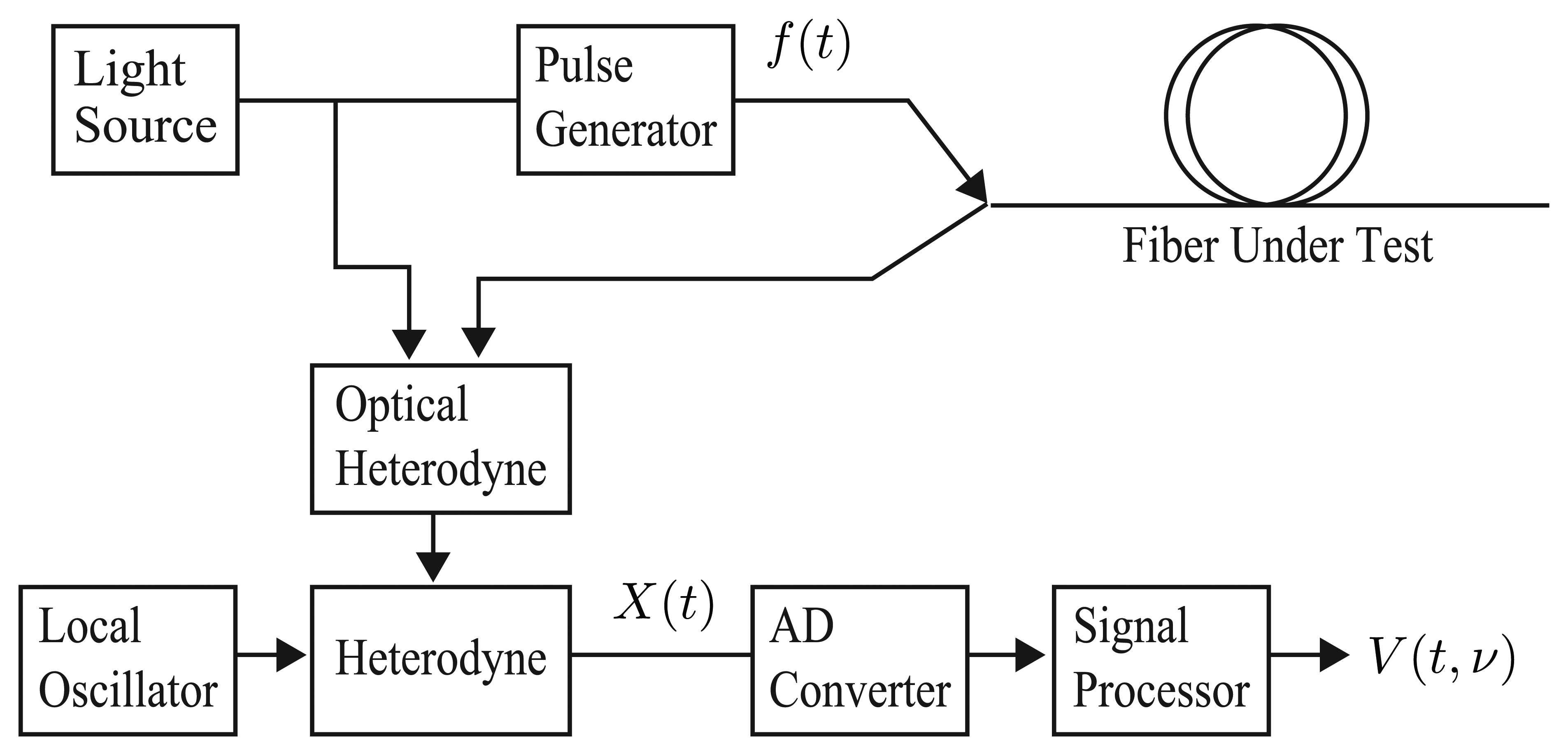
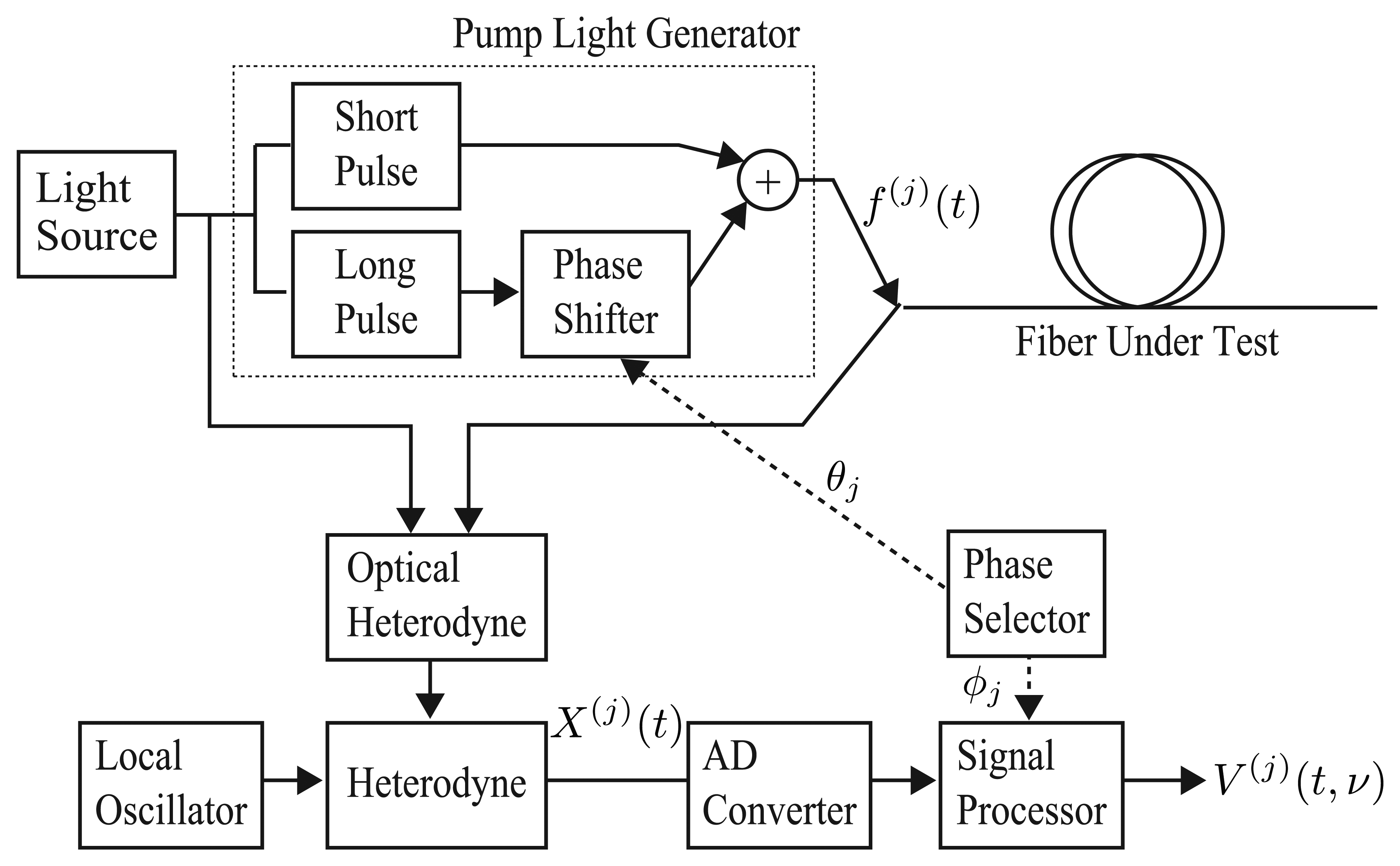
A BOTDR system is shown in Figure 1. The light from the light source is divided into a pump pulse and a reference continuous wave. In an optical fiber, the acoustic waves are always excited by thermal fluctuation and the pump pulse is scattered by the acoustic waves in all parts of the fiber. Since the acoustic waves move with the sound velocity of the medium, the backscattered light has a Doppler shift, which is called a Brillouin frequency shift (BFS). As the sound velocity changes in proportion to the change in strain or temperature in each position of the fiber, the BFS also changes in proportion to them. In BOTDR, the backscattered light is heterodyned with the reference wave and the spectrum of the interfering light; i.e., the Brillouin spectrum is obtained. The BFS is estimated from the Brillouin spectrum as its center frequency. Since the round-trip time of the light corresponds to the position in the fiber, the BFS at each position in the fiber is obtained. Thus, distributed sensing of strain and temperature is possible using the Brillouin scattered light.

2.2. Basic Equations of BOTDR

Brillouin scattering in optical fiber is described by the following equations [16–18]:

$$\left(\frac{1}{{\upsilon }_{\text{g}}}\frac{\partial }{\partial t}+\frac{\partial }{\partial z}+\frac{\alpha }{2}\right)E_{\text{p}}=i\kappa \rho E_{\text{s}}$$

(1)

$$\left(\frac{1}{{\upsilon }_{\text{g}}}\frac{\partial }{\partial t}-\frac{\partial }{\partial z}+\frac{\alpha }{2}\right)E_{\text{s}}=i\kappa \rho *E_{\text{p}}$$

(2)

$$\frac{\partial \rho }{\partial t}+\left(\frac{{\Gamma }_{\text{B}}}{2}+2\pi i{\nu }_{\text{B}}(z)\right)\rho =i\wedge E_{\text{p}}{E}_{\text{s}}^{*}+R(z,t)$$

(3)

where E_p, E_s and ρ are complex amplitudes of a pump light, a backscattered light and an acoustic wave, respectively, κ and Λ are coupling coefficients, υ_g is the light speed in the fiber, α is the fiber loss factor and superscript * denotes a complex conjugate. Γ_B is the linewidth of the acoustic wave spectrum and ν_B(z) denotes the BFS at position z. Here, the spectral linewidth is defined by the full width at half maximum.

Random force R(z, t) is a circular symmetric complex white noise that is white both in space and time; i.e., it is characterized by E [R(z, t)R*(z′, t′)] = Qδ(z−z′)δ(t−t′), where E[·] stands for expectation and Q is a constant. The two terms in the right-hand side (RHS) of Equation (3) correspond to stimulated and spontaneous Brillouin scattering, respectively Under usual BOTDR conditions, as analyzed in a previous paper [19], the largest part of the measured spectrum arises from spontaneous scattering, and the stimulated scattering term can be neglected. Moreover, then, since it becomes |E_s| ≪ |E_p|, the RHS of Equation (1) can be neglected. Therefore, BOTDR is described by the following equations:

$$\left(\frac{1}{{\upsilon }_{\text{g}}}\frac{\partial }{\partial t}+\frac{\partial }{\partial z}+\frac{\alpha }{2}\right)E_{\text{p}}=0$$

(4)

$$\left(\frac{1}{{\upsilon }_{\text{g}}}\frac{\partial }{\partial t}-\frac{\partial }{\partial z}+\frac{\alpha }{2}\right)E_{\text{s}}=i\kappa \rho *E_{\text{p}}$$

(5)

$$\frac{\partial \rho }{\partial t}+(\Gamma +2\pi i{\nu }_{\text{B}}(z))\rho =R(z,t)$$

(6)

The boundary conditions of E_p(z, t) and E_s(z, t) are given by:

$$E_{\text{p}}(0,t)=\sqrt{\frac{P_{\text{p}}}{A_{\text{eff}}}}f(t)$$

(7)

$$E_s\left(z,\frac{z}{{\upsilon }_g}\right)=0$$

(8)

where P_p and f(t) denote the power and shape function of the pump pulse injected into an optical fiber, respectively, A_eff is the effective core area of a fiber and Γ = Γ_B/2 is set.

2.3. Analytical Solution to the BOTDR Equations

The solution to last section's BOTDR equations can be represented analytically. For simplicity, assuming that the fiber loss is small, we set α = 0.

First, the solution to Equation (1) under boundary Condition Equation (7) is represented as:

$$E_{\text{p}}(z,t)=\sqrt{\frac{P_{\text{p}}}{A_{\text{eff}}}}f\left(t-\frac{z}{{\upsilon }_g}\right)$$

(9)

Next, the stationary solution to Equation (6) is represented as:

$$\rho (z,t)={\int }_{-\infty }^t{e}^{-(\Gamma +2\pi i{\nu }_B(z))(t-s)}R(z,s)ds$$

(10)

whose autocorrelation function is given by:

$$E[\rho (z,t){\rho }^{*}(z^{\prime },t^{\prime })]=\frac{Q}{2\Gamma }\delta (z-z^{\prime })e^{-2\pi i{\nu }_{\text{B}}(z)(t-t^{\prime })}{e}^{-\Gamma |t-t^{\prime }|}$$

(11)

Then, substituting (9) and (10) into (5) and solving it under Condition (8), we obtain:

$$E_s(z,t)=i{\kappa }_1{\int }_z^{L_f}f\left(t-\frac{2z^{\prime }-z}{{\upsilon }_{\text{g}}}\right){\rho }^{*}\left(z^{\prime },t-\frac{z^{\prime }-z}{{\upsilon }_{\text{g}}}\right)d{z}^{\prime }$$

(12)

where ${\kappa }_1=\sqrt{P_{\text{p}}/A_{\text{eff}}}\kappa$ and L_f is the length of the fiber.

The backscattered light returned to the input end of an optical fiber in BOTDR is represented as:

$$X(t)\stackrel{\text{def}}{=}{E}_s(0,t)=i{\kappa }_1{\int }_0^{L_{\text{f}}}f\left(t-\frac{2z}{{\upsilon }_{\text{g}}}\right){\zeta }^{*}(z,t)dz$$

(13)

where we set ζ(z, t) ≡ ρ(z, t − z/υ_g), which has the same statistical property as ρ(z, t); i.e.,

$$E[\zeta (z,t){\zeta }^{*}(z^{\prime },t^{\prime })]=\frac{Q}{2\Gamma }\delta (z-z^{\prime })e^{-2\pi i{\nu }_{\text{B}}(z)(t-t^{\prime })}{e}^{-\Gamma |t-t^{\prime }|}$$

(14)

holds. We note that X(t) becomes a circular complex Gaussian (ccG) process with mean zero. The component of this signal with frequency ν is obtained by:

$$\begin{array}{ll}Y(t,\nu )\hfill & =c_{Y}h(t)*[X(t)e^{-2\pi i\nu t}]\hfill \\ \hfill & =i{\kappa }_2{\int }_{-\infty }^{\infty }h(t-\tau )e^{-2\pi i\nu \tau }{\int }_0^{L_{\text{f}}}f\left(\tau -\frac{2z}{{\upsilon }_g}\right)\zeta *(z,\tau )\mathit{\text{dzd}}\tau \hfill \end{array}$$

(15)

where c_Y is a constant, h(t) is an impulse response of a low-pass filter and * denotes a convolution, and we set κ₂ = c_Y κ₁. Y(t, ν) also becomes a ccG process with a mean of zero as X(t).

2.4. Brillouin Spectrum and Point Spread Function

The Brillouin spectrum obtained by one measurement of BOTDR is represented as:

$$V(t,\nu )={\left|Y(t,\nu )\right|}^2$$

(16)

Since BOTDR's signal source is thermally excited acoustic waves, its spectrum fluctuates even without observation noise. Although the spectrum is averaged by many replicate measurements, we must suppress the fluctuation for one measurement.

Since Y(t, ν) is a ccG process, V(t, ν) becomes a random variable with an exponential distribution for each t and ν, so its variance equals the square of its expectation:

$$E{[V(t,\nu )-EV(t,\nu )]}^2={\left(EV(t,\nu )\right)}^2$$

(17)

To obtain a smooth spectrum, measurements are performed many times and the spectrums are accumulated or averaged. Therefore, the Brillouin spectrum obtained by measurements is considered to be expectation EV(t, ν).

We can calculate the expectation of V(t, ν) by using the statistical property of Equation (11) as:

$$EV(t,\nu )={\gamma }_{\text{R}}L(t,\nu )\stackrel{t,\nu }{*}\mathrm{\Psi }(t,\nu )$$

(18)

where ${\gamma }_{\text{R}}={\upsilon }_{\text{g}}{\kappa }_2^{2}Q/2{\Gamma }^2$ is a constant and $\stackrel{t,\nu }{*}$ denotes a two-dimensional convolution with respect to t and ν. Functions L(t, ν) and ψ(t, ν) are defined by:

$$L(t,\nu )=\frac{{\Gamma }^2}{{\Gamma }^2+{\left(2\pi (\nu -{\nu }_B({\upsilon }_{\text{g}}t/2)\right)}^2}$$

(19)

$$\mathrm{\Psi }(t,\nu )={\left|{\mathcal{F}}_{\tau }[f(\tau )h\left(t-\tau \right)]\right|}^2$$

(20)

respectively, where denotes the Fourier transform with respect to τ. Equation (18) is derived in Appendix A.

We note that L(t, ν) is a time-varying Lorentzian spectrum and is determined only by the characteristics of an optical fiber, whereas ψ(t, ν) depends on the sensing mechanism of BOTDR. Since Equation (18) implies that function, ψ(t, ν), obscures the details of L(t, ν), we refer to Ψ(t, ν) as a point spread function (PSF).

2.5. Performance Limit of BOTDR

Though the ideal Brillouin spectrum is the Lorentzian spectrum, the observed Brillouin spectrum is spread by the PSF. Therefore, it is desirable for the PSF to have a shape close to a two-dimensional δ-function; that is, narrow in both time and frequency directions. However, by the following uncertainty relation (see Appendix B):

$$2{\mathrm{\Delta }}_{\text{T}}·2{\mathrm{\Delta }}_{\text{F}}\ge \frac{2}{\pi }$$

(21)

the product of time and frequency widths of the PSF cannot be reduced below a certain value. Since the time width corresponds to the spatial resolution, there is a limit, in principle, to improving both spatial and frequency resolution simultaneously through one measurement with whatever pump pulses and low-pass filters are used.

3. BOTDR by the Synthetic Approach

To overcome the resolution limitation of conventional BOTDR described in the previous section, a synthetic spectrum approach, which we refer to as synthetic BOTDR (S-BOTDR), is proposed.

3.1. Elements of the Point Spread Function

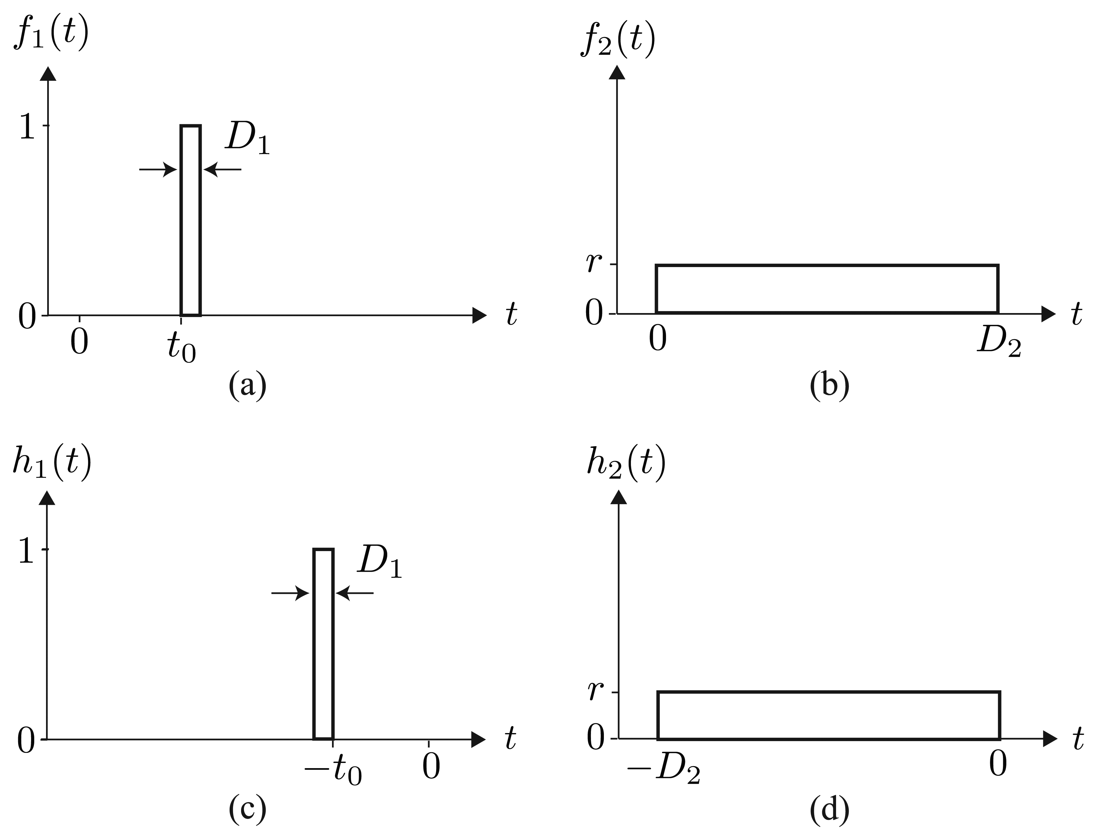
We consider a short pulse, f₁(t), and a long pulse, f₂(t), as elements of composite pump light:

$$f_1(t)=I_{[t_0,t_0+D_1]}(t)$$

(22)

$$f_2(t)=r{I}_{[0,D_2]}(t)$$

(23)

where I_[a,b] is the definition function of interval [a, b], D₁ and D₂ are the pulse widths of two pulses and r is the amplitude ratio of the two pulses. The start time of the short pulse is denoted by t₀.

Similar to the PPP-BOTDA method [8,9], D₁ is set as less than the spatial resolution to be attained and D₂ is taken as sufficiently longer than the acoustic wave lifetime, 2/Γ_B, say about 9 ns, to improve frequency resolution. A low-pass filter is also composed of two elements, each of which is a matched filter of short or long pulses:

$$h_1(t)=f_1(-t)$$

(24)

$$h_2(t)=f_2(-t)$$

(25)

By using the above elements, a pump light and a low-pass filter are composed as:

$$f_{\theta }(t)=f_1(t)+e^{i\theta }{f}_2(t)$$

(26)

$$h_{\varphi }(t)=h_1(t)+e^{i\varphi }{h}_2(t)$$

(27)

where θ and ϕ are the phase differences of the two elements. The PSF corresponding to the composite pump light and low-pass filter becomes:

$$\begin{array}{ll}{\mathrm{\Psi }}_{\theta ,\varphi }(t,\nu )\hfill & ={\left|{\mathcal{F}}_{\tau }\{f_{\theta }(\tau )h_{\varphi }(t-\tau )\}\right|}^2\hfill \\ \hfill & ={\left|F_{11}\right|}^2+{\left|F_{12}\right|}^2+{\left|F_{21}\right|}^2+{\left|F_{22}\right|}^2+2\Re [e^{-i\theta }(F_{11}{F}_{21}^{*}+F_{12}{F}_{22}^{*})\hfill \\ \hfill & +e^{-i\varphi }(F_{11}{F}_{12}^{*}+F_{21}{F}_{22}^{*})+e^{-i(\theta -\varphi )}{F}_{12}{F}_{21}^{*}+e^{-i(\theta +\varphi )}{F}_{11}{F}_{22}^{*}]\hfill \end{array}$$

(28)

where ℜ[·] denotes the real part, and the RHS is composed of functions:

$$\begin{array}{ll}{F}_{kl}\hfill & \equiv F_{kl}(t,\nu )={\mathcal{F}}_{\tau }[f_k(\tau )h_l(t-\tau )]\hfill \\ \hfill & \begin{array}{ll}={\mathcal{F}}_{\tau }[f_k(\tau )f_l(\tau -t)],\hfill & k,l=1,2\hfill \end{array}\hfill \end{array}$$

(29)

The spreadness of function F_kl has the following features, due to the difference in pulse widths of the two pulses (see also Figure 3):

$$\begin{array}{cc}{F}_{11}:& \text{small in time and large in frequency},\\ F_{12}\text{and}{F}_{21}:& \text{large in both time and frequency},\\ F_{22}:& \text{large in time and small in frequency}.\end{array}$$

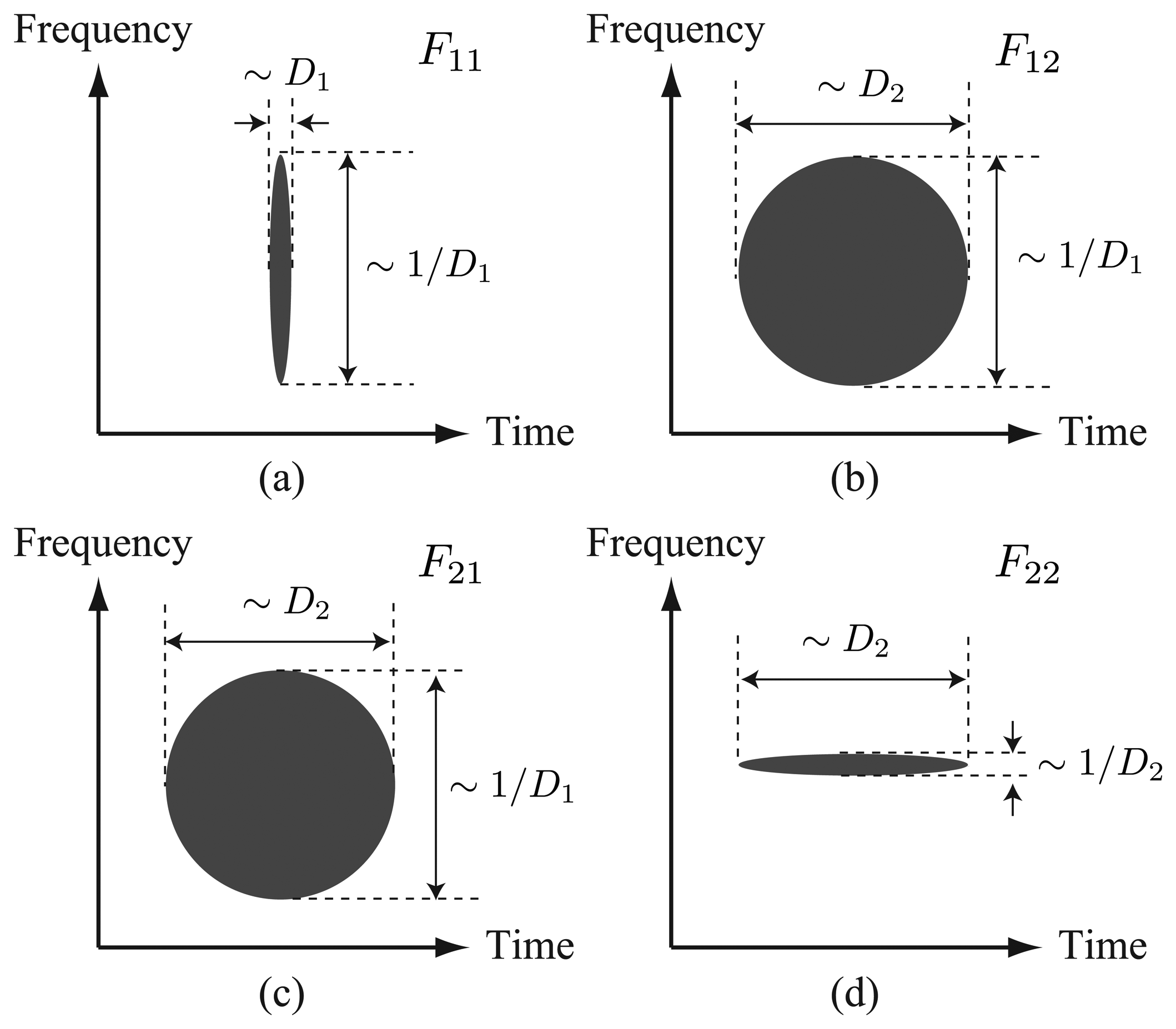
Therefore, among the terms of the RHS of Equation (28), only the term, $F_{11}{F}_{22}^{*}$, has the ideal property that it is localized both in time and frequency, and the other terms are undesired elements for the BOTDR measurement.

3.2. PSF by the Synthetic Approach

To extract only element $\Re (F_{11}{F}_{22}^{*})$ from the PSF, we prepare p phase pairs ((θ_j, ϕ_j), j = 1, 2, ⋯, p) and p pairs of pump lights and low-pass filters:

$$f^{(j)}(t)=f_1(t)+e^{i{\theta }_j}{f}_2(t)$$

(30)

$$\begin{array}{r}\hfill h^{(j)}(t)=h_1(t)+e^{i{\varphi }_j}{h}_2(t)\\ \hfill j=1,2,\cdots ,p\end{array}$$

(31)

The Brillouin spectrum and the PSF obtained by using f^(j)(t) and h^(j)(t) are denoted by V^(j)(t, ν) and Ψ^(j)(t, ν), respectively The synthetic spectrum is defined as:

$$V_{\text{S}}(t,\nu )=\sum _{j=1}^p{c}_j{V}^{(j)}(t,\nu )$$

(32)

where c_j, j = 1, 2, ⋯, p are weighting coefficients. The corresponding synthetic PSF becomes:

$${\mathrm{\Psi }}_{\text{S}}(t,\nu )=\sum _{j=1}^p{c}_j{\mathrm{\Psi }}^{(j)}(t,\nu )$$

(33)

The j-th PSF is represented as:

$${\mathrm{\Psi }}^{(j)}(t,\nu )={\left|{\mathcal{F}}_{\tau }[f^{(j)}(\tau )h^{(j)}(t-\tau )]\right|}^2$$

(34)

which is expanded as:

$$\begin{array}{ll}{\mathrm{\Psi }}^{(j)}(t,\nu )=\hfill & {\left|F_{11}\right|}^2+{\left|F_{12}\right|}^2+{\left|F_{21}\right|}^2+{\left|F_{22}\right|}^2\hfill \\ \hfill & +2\Re [e^{-i{\theta }_j}(F_{11}{F}_{21}^{*}+F_{12}{F}_{22}^{*})+e^{-i{\varphi }_j}(F_{11}{F}_{12}^{*}+F_{21}{F}_{22}^{*})\hfill \\ \hfill & +e^{-i({\theta }_j-{\varphi }_j)}{F}_{12}{F}_{21}^{*}+e^{-i({\theta }_j+{\varphi }_j)}{F}_{11}{F}_{22}^{*}\hfill \end{array}$$

(35)

If the following relation holds by combining the PSFs, an ideal PSF is obtained.

$${\mathrm{\Psi }}_{\text{S}}(t,\nu )=2p\Re [F_{11}{F}_{22}^{*}]$$

(36)

This problem is equivalent to finding θ_j, ϕ_j, c_j, j = 1, 2, ⋯, p that satisfy:

$$\left(\begin{array}{cccc}1& 1& \cdots & 1\\ e^{-i{\theta }_1}& e^{-i{\theta }_2}& \cdots & e^{-i{\theta }_p}\\ e^{-i{\varphi }_1}& e^{-i{\varphi }_2}& \cdots & e^{-i{\varphi }_p}\\ e^{-i({\theta }_1-{\varphi }_1)}& e^{-i({\theta }_2-{\varphi }_2)}& \cdots & e^{-i({\theta }_p-{\varphi }_p)}\\ e^{-i({\theta }_1+{\varphi }_1)}& e^{-i({\theta }_2+{\varphi }_2)}& \cdots & e^{-i({\theta }_p+{\varphi }_p)}\end{array}\right)\left(\begin{array}{c}{c}_1\\ c_2\\ ⋮\\ c_p\end{array}\right)=\left(\begin{array}{l}0\hfill \\ 0\hfill \\ 0\hfill \\ 0\hfill \\ p\hfill \end{array}\right)$$

(37)

Though the general solution has not been obtained, the following solution with p = 4 is at least a solution to Equation (37):

$$\begin{array}{ccc}\left(\begin{array}{c}{\theta }_1\\ {\theta }_2\\ {\theta }_3\\ {\theta }_4\end{array}\right)=\left(\begin{array}{c}0\\ \pi /2\\ \pi \\ 3\pi /2\end{array}\right),& \left(\begin{array}{l}{\varphi }_1\hfill \\ {\varphi }_2\hfill \\ {\varphi }_3\hfill \\ {\varphi }_4\hfill \end{array}\right)=\left(\begin{array}{c}0\\ 3\pi /2\\ 0\\ \pi /2\end{array}\right),& \left(\begin{array}{c}{c}_1\\ c_2\\ c_3\\ c_4\end{array}\right)\end{array}=\left(\begin{array}{c}-1\\ 1\\ -1\\ 1\end{array}\right)$$

(38)

Hereafter, we use this solution.

The PSF by the synthetic approach is represented as:

$${\mathrm{\Psi }}_S(t,\nu )=8\Re [F_{11}{F}_{22}^{*}]$$

(39)

and is concentrated around the origin in both the time and frequency directions, as shown in the previous section. However, in addition to this, its two-dimensional integral in the time-frequency space must be a certain positive value to approximate a two-dimensional δ-function. The two-dimensional integral of the synthetic PSF of Equation (39) becomes:

$${\int }_{-\infty }^{\infty }{\int }_{-\infty }^{\infty }{\mathrm{\Psi }}_{\text{S}}(t,\nu )d\nu dt=8{\left({\int }_{-\infty }^{\infty }{f}_1(t)f_2(t)dt\right)}^2$$

(40)

If two pulses are separated in time, this integral becomes zero, and if they overlap partially, the integral is proportional to the width of the overlapping parts. To maximize the integral, the short pulse must be included in the long pulse, and the integral becomes $8r^2{D}_1^2$.

For two pulses of Equations (22) and (23), the synthetic PSF becomes:

$${\mathrm{\Psi }}_S(t,\nu )=8r^{2}cos\pi (D_2-D_1-2t_0)\nu \frac{sin\pi (D_1-|t|)\nu }{\pi \nu }\frac{sin\pi (D_2-|t|)\nu }{\pi \nu }{I}_{[-D_1,D_1]}(t)$$

(41)

If D₁ is sufficiently small and D₂ is sufficiently large, the PSF is approximated as:

$${\mathrm{\Psi }}_{\text{S}}(t,\nu )\approx 8r^2{D}_1^2\delta (\nu )$$

(42)

and the synthetic spectrum is approximated as:

$$E{V}_S(t,\nu )\approx 8r^2{D}_1^2{\gamma }_{R}L(t,\nu )$$

(43)

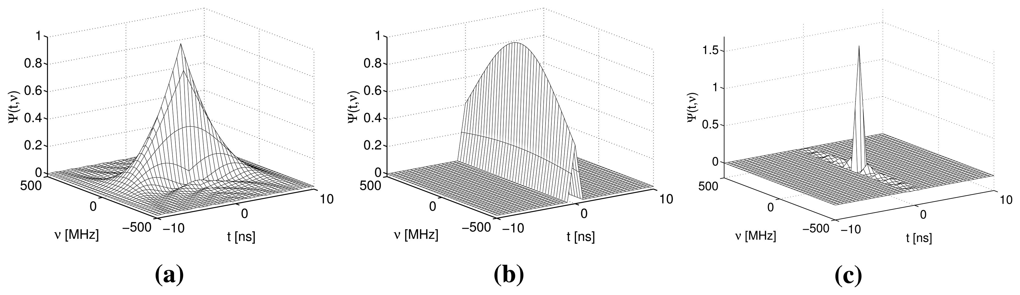
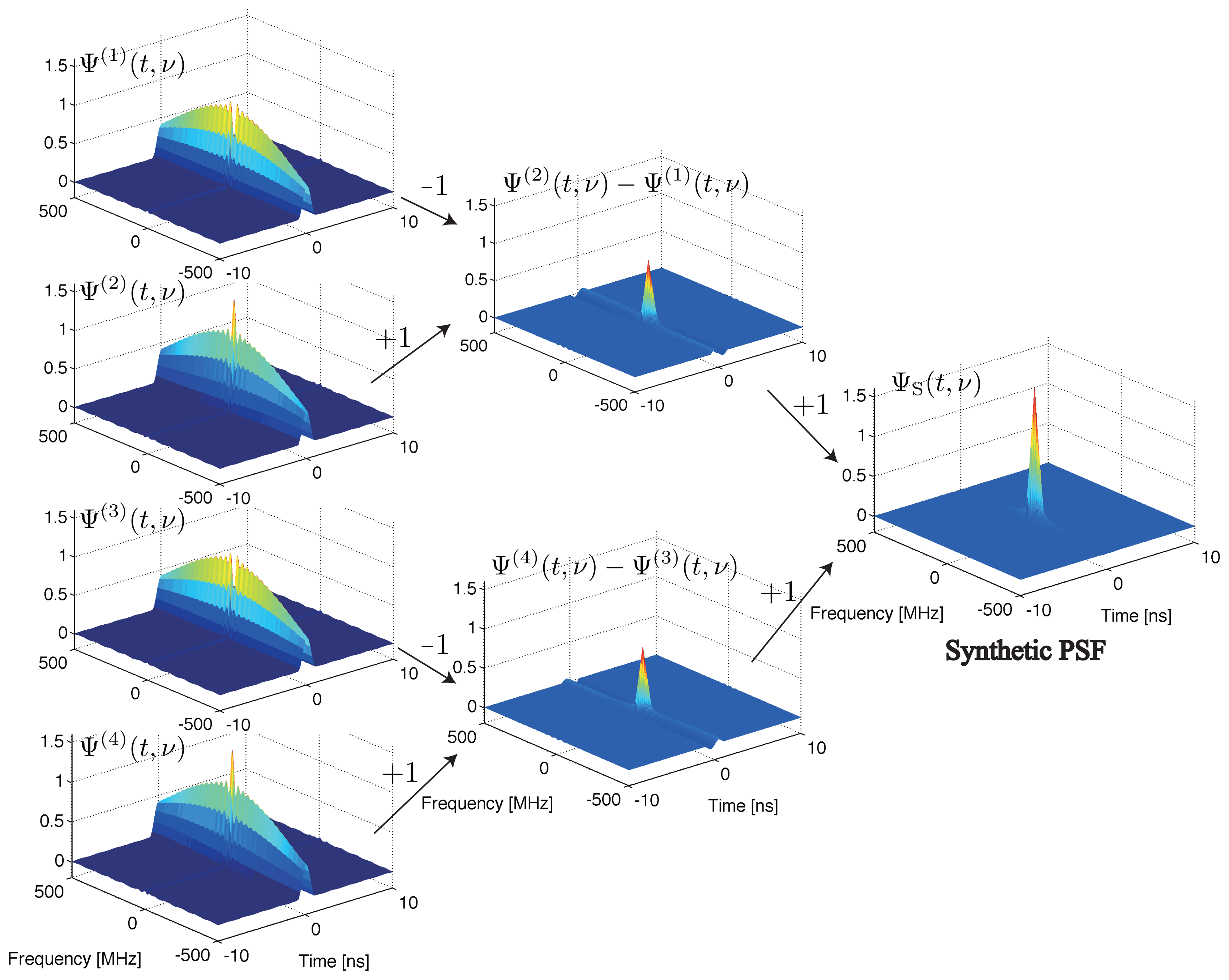
The PSFs for a conventional BOTDR and S-BOTDR are plotted in Figure 4. While the PSF of the conventional BOTDR spreads in either the time or frequency direction, that of S-BOTDR is concentrated at the origin and approximates a δ-function. To clarify the mechanism of generating such a δ-like function, the composition of the synthetic PSF is shown in Figure 5. Although each of the PSF, Ψ^(j), j = 1, 2, 3, 4, concentrates in the time direction, it is spread in the frequency direction. This spreading is partially suppressed with two-by-two combination, Ψ⁽²⁾ − Ψ⁽¹⁾ and Ψ⁽⁴⁾ − Ψ⁽³⁾, and is completely suppressed with the use of all PFS elements.

3.3. S-BOTDR System

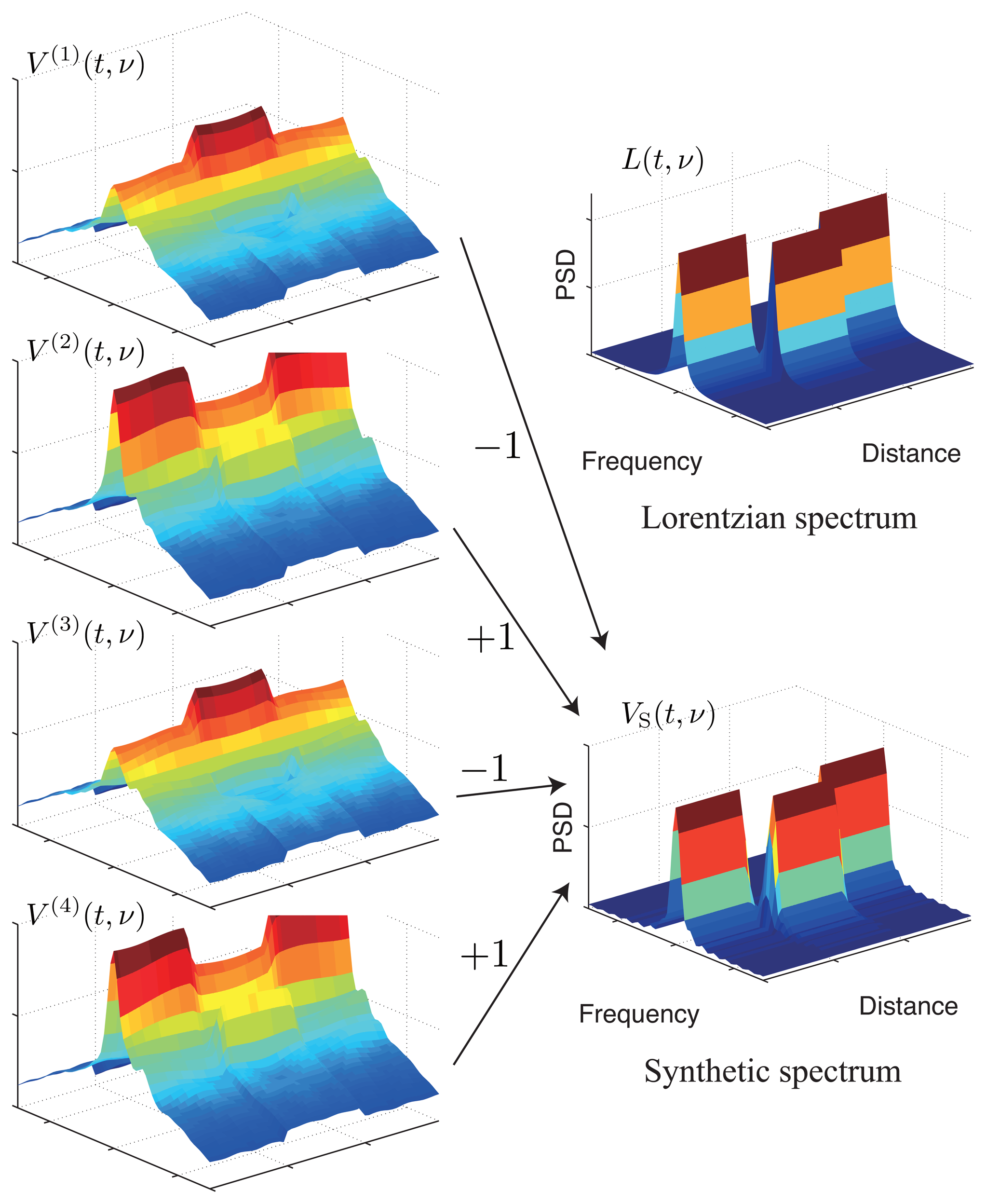
As shown in the analysis of the previous section, the synthetic Brillouin spectrum has the ideal property of being close to a Lorentzian spectrum. An S-BOTDR system for obtaining the synthetic Brillouin spectrum is constructed as shown in Figure 6. The composition of the synthetic Brillouin spectrum is followed by Equation (32) and is illustrated in Figure 7. Although the spectrum of each measurement exhibits high spatial resolution, it is considerably different from the Lorentzian spectrum. Only the combination of all four spectrums produces the Lorentzian spectrum.

The ideal property described in the previous section is for the expectation of the synthetic Brillouin spectrum. Achieving this property requires averaging or summing of the spectrums obtained by a number of measurements.

3.4. Parameter Selection for S-BOTDR

The pump lights of S-BOTDR are composed of short and long pulses and include parameters t₀ and r: t₀ is the difference of pulse start times and r is the amplitude ratio of the two pulses. These parameters affect the performance of S-BOTDR.

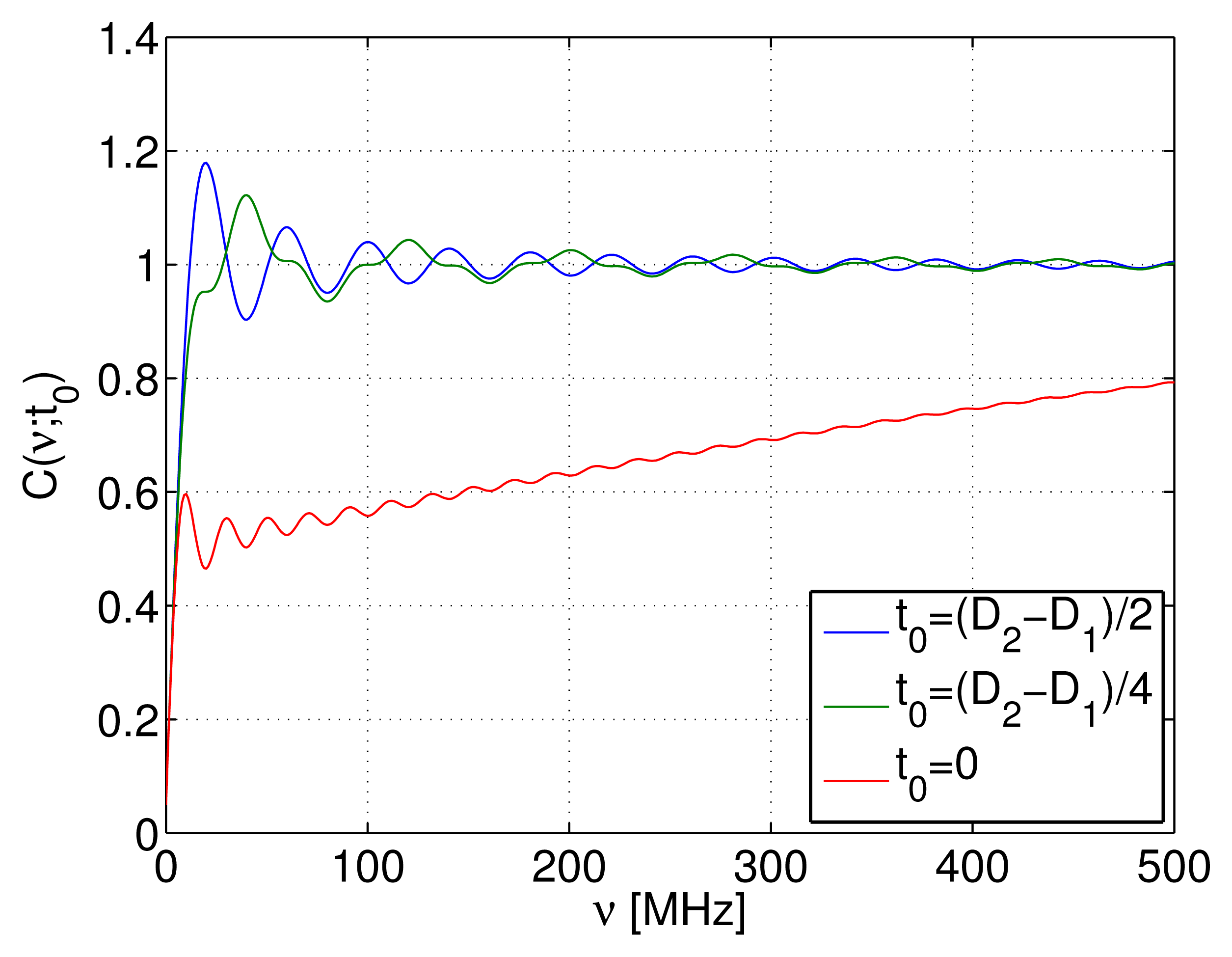
Selection of t₀ If the short pulse is included in the long pulse, i.e., if 0 ≤ t₀ ≤ D₂ − D₁, the integral of Equation (40) takes the maximum value. In addition, the value of t₀ affects the concentration of the PSF near the origin. The degree of concentration is estimated by the integral:

$$C(\nu ;t_0){\int }_{-\nu }^{\nu }{\int }_{-\infty }^{\infty }\mathrm{\Psi }(t,{\nu }^{\prime })\mathit{\text{dtd}}{\nu }^{\prime }/(8r^2{D}_1^2)$$

(44)

If C(ν; t₀) approaches one for small ν, the PSF is considered to be concentrated near the origin of the frequency axis.

The values of C(ν; t₀) are plotted for different t₀'s in Figure 8. Here, for t₀ = (D₂ − D₁)/2, the short pulse is located at the center of the long pulse; for t₀ = 0, the short pulse is at the edge of the long pulse, and the medium case is t₀ = (D₂ − D₁)/4. From Figure 8, we find that when the short pulse is located at the edge of the long pulse, the degree of concentration is reduced. Thus, we adopt t₀ = (D₂ − D₁)/2.

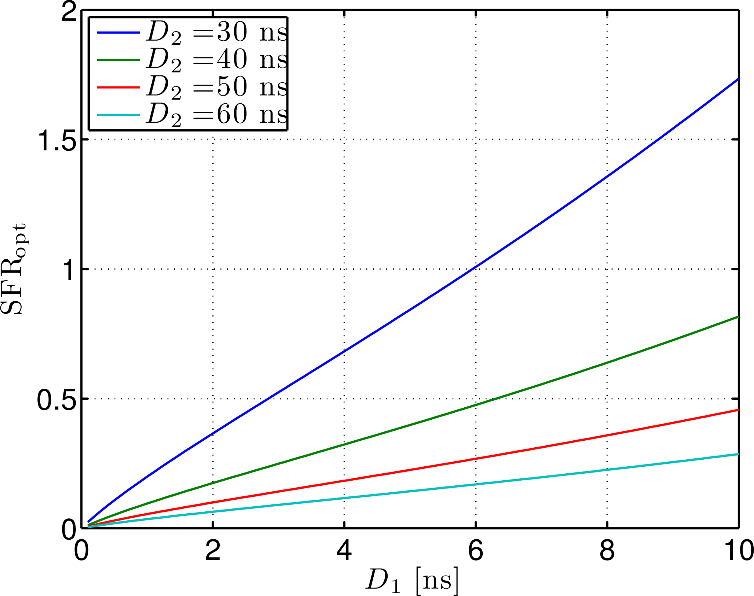
Selection of r It is desirable for S-BOTDR to suppress the synthetic spectrum's fluctuation as much as possible while keeping the peak level high. To meet these requirements, we define the signal-to-fluctuation ratio (SFR) as:

$$\text{SFR}=\frac{{\mu }_{\text{peak}}^2}{{\sigma }_{\text{peak}}^2}$$

(45)

where μ_peak and ${\sigma }_{\text{peak}}^2$ are the mean and the variance of the synthetic spectrum at the peak, respectively As shown in Appendix C, the SFR is represented explicitly as a function of r, and the optimal r, which maximizes the SFR, is given by:

$$r_{\mathit{\text{opt}}}={\left(\frac{{\left(\Gamma D_1\right)}^2-2\Gamma D_1+2(1-e^{-\Gamma D_1})}{{\left(\Gamma D_2\right)}^2-2\Gamma D_2+2(1-e^{-\Gamma D_2})}\right)}^{1/4}$$

(46)

Numerical examples of r_opt are shown in

Table 1. Numerical examples of r_opt.

D1 [ns]	D2 (ns)
	30	40	50	60
1	0.0896	0.0750	0.0656	0.0589
2	0.1499	0.1254	0.1096	0.0985
3	0.2020	0.1690	0.1477	0.1327
4	0.2493	0.2085	0.1823	0.1638
5	0.2930	0.2451	0.2143	0.1925
6	0.3342	0.2795	0.2444	0.2195
7	0.3731	0.3121	0.2728	0.2451
8	0.4102	0.3431	0.3000	0.2695
9	0.4458	0.3728	0.3260	0.2929
10	0.4800	0.4014	0.3510	0.3153

. We used the optimal r in simulations and experiments.

The SFR of S-BOTDR is obtained by substituting (46) into (76) in Appendix C. The SFR values for various D₁ and D₂ are plotted in Figure 9. From this figure, we find that SFR is nearly proportional to D₁ for fixed D₂. On the other hand, BFS estimation error variance is inversely proportional to SFR [20]. Therefore, the BFS estimation error variance is nearly proportional to 1/D₁.

4. Evaluation by Simulation

Numerical simulations were performed to verify the S-BOTDR and compare it with the conventional BOTDR. The condition of the optical fiber is shown in Figure 10. In the figure, an assumed BFS is shown in (a) and the corresponding Lorentzian spectrum is shown in (b). Simulation results are shown in Figures 11, 12, and 13. The parameter values for processing are as follows:

• Conventional BOTDR (Figures 11 and 12)

  Pulse width is D = 10 and 1 ns.

• S-BOTDR (Figure 13)

  Pulse widths are D₁ = 1 ns for a short pulse and D₂ = 50 ns for a long pulse. The amplitude ratio is r = 0.066. The short pulse is located at the center of the long pulse.

All results were obtained by summing 2¹² trials. For conventional BOTDR with a 10-ns pulse in Figure 11, the linewidth of the spectrum was small and smooth; however, spatial resolution was inferior and could not detect any interval less than 50 cm. For the conventional BOTDR with a 1-ns pulse in Figure 12, because the linewidth of the spectrum was quite large (about 1 GHz), the estimation accuracy of the BFS was inferior. In the case of the S-BOTDR in Figure 13, the Brillouin spectrum was close to the Lorentzian spectrum; hence, accurate BFS estimates were obtained. Thus, S-BOTDR has a high-resolution capability exceeding that of conventional BOTDR.

The simulation was performed using the exact values of the input parameters. In an actual situation, these parameters are, however, subject to errors. As in S-BOTDR four measurements are combined, the input light amplitude fluctuation and phase-setting errors become issues of concern. Among them, the light amplitude fluctuation becomes negligible by averaging many replicate measurements. The errors in the phase differences between short and long elements are, on the other hand, anticipated. We performed a series of additional simulations in which the phase differences were subject to random errors. The results clearly demonstrated that they did not affect the spatial resolution, while the BFS estimation error increased only slightly, even if phase errors as high as 40 degrees were applied.

5. Experimental Verification

We performed BOTDR and S-BOTDR experiments using a test fiber. We constructed a test fiber by connecting two kinds of fibers: A and B (Figure 14a). The BFS between fibers A and B differs, and the difference corresponds to a strain of 1,200 μ∊. In the experiments, fibers A and B are considered strained fibers and strain-free fibers, respectively. The replicate measurement numbers were 2¹⁶ in all cases. The experimental result for BOTDR is shown in Figure 15. The pulse width of the pump light for BOTDR was 5 ns. Strain estimates and the Brillouin spectrum at the 5-m strain interval are plotted in Figure 15a,b, respectively. The linewidth of the Brillouin spectrum exceeded 360 MHz (Figure 15b). Although intervals larger than or equal to one meter were accurately detected, the strain estimates of the other intervals differed from the true values (Figure 15a).

We performed S-BOTDR experiments using the following combination of short and long elements for the pump light and the low-pass filter:

• Case 1 D₁ = 7.8 ns, D₂ = 60 ns, r = 0.26

• Case 2 D₁ = 2.7 ns, D₂ = 50 ns, r = 0.14

• Case 3 D₁ = 1.6 ns, D₂ = 50 ns, r = 0.093

Here, the values of r were determined to be the optimal values. The strain estimates in each case are plotted in Figure 16a–c. We attained a spatial resolution of 50 cm in Case 1, 20 cm in Case 2 and 10 cm in Case 3. Figures 16a-c also indicate that the fluctuation of estimates increases as D₁ becomes small. This is because the estimation error variance is nearly proportional to 1/D₁, as is described in Section 3.4. Therefore, some compromise is required to select small D₁. The synthetic spectrums at the 5-m strain interval are shown in Figure 16d,e. In all cases, their linewidths were less than 40 MHz. This is because the linewidth of the synthetic spectrums is determined by the reciprocal of the long pulse's length. These experimental results prove that we attained 10-cm spatial resolution that exceeds the limit of conventional BOTDR.

6. Conclusions

We showed that conventional BOTDR has, in principle, a resolution limit and proposed a synthetic spectrum approach, referred to as S-BOTDR, to overcome this limit. S-BOTDR uses composite pump lights and low-pass filters that are composed of short and long elements with different phases. Four BOTDR measurements are performed using four specific pairs of phases. By combining four Brillouin spectrums with specific weights, an ideal spectrum is obtained. The spectrum is close to the Lorentzian spectrum, and the resolution limit, in principle, disappears. We experimentally evaluated S-BOTDR and proved that we attained a 10-cm resolution that exceeds the resolution limit of conventional BOTDR.

References

- Horiguchi, T.; Kurashima, T.; Tateda, M. Tensile strain dependence of Brillouin frequency shift in silica optical fibers. IEEE Photon. Technol. Lett. 1989, 1, 107–108. [Google Scholar]
- Horiguchi, T.; Shimizu, K.; Kurashima, T.; Tateda, M.; Koyamada, Y. Development of a distributed sensing technique using Brillouin scattering. J. Lightw. Technol. 1995, 13, 1296–1302. [Google Scholar]
- Horiguchi, T.; Tateda, M. BOTDA–Nondestructive measurement of single-mode optical fiber attenuation characteristics using Brillouin interaction: Theory. J. Lightw. Technol. 1989, 7, 1170–1176. [Google Scholar]
- Kurashima, T.; Tsuneo Horiguchi Hisashi Izumita, S.I.F.; Koyamada, Y. Brillouin optical-fiber time domain reflectometry. IEICE Trans. Commun. 1993, E76-B, 382–390. [Google Scholar]
- Horiguchi, T.; Shimizu, K.; Kurashima, T.; Koyamada, Y. Advances in distributed sensing techniques using Brillouin scattering. Proceedings of the SPIE, Munich, Germany, 19 June 1995; Volume 2507, pp. 126–137.
- Kurashima, T.; Tateda, M.; Horiguchi, T.; Koyamada, Y. Performance improvement of a combined OTDR for distributed strain and loss measurement by randomizing the reference light polarization state. IEEE Photon. Technol. Lett. 1997, 9, 360–362. [Google Scholar]
- Bao, X.; Brown, A.; DeMerchant, M.; Smith, J. Characterization of the Brillouin-loss spectrum of single-mode fibers by use of very short (10-ns) pulses. Opt. Lett. 1999, 24, 510–512. [Google Scholar]
- Kishida, K.; Nishiguchi, K. Pulsed pre-pump method to achieve cm-order spatial resolution in Brillouin distributed measuring technique Technical Report of IEICE, OFT2004-47 (2004-10). 2004, 15–20.
- Nishiguchi, K.; Kishida, K. Perturbation analysis of stimulated Brillouin scattering in an optical fiber and a resolution improvement method. Proceedings of the 37th ISCIE International Symposium on Stochastic Systems Theory and Its Applications, (SSS2005), Osaka, Japan, 28–29 October 2005; pp. 232–239.
- Zou, L.; Bao, X.; Wan, Y.; Chen, L. Coherent probe-pump-based Brillouin sensor for centimeter-crack detection. Optics Letters 2005, 30, 370–372. [Google Scholar]
- Brown, A.W.; Colpitts, B.G.; Brown, K. Dark-pulse Brillouin optical time-domain sensor with 20-mm spatial resolution. J. Lightw. Technol. 2007, 25, 381–386. [Google Scholar]
- Thévenaz, L.; Foaleng, S.M. Distributed fiber sensing using Brillouin echoes. Proceedings of the 19th Internetional Conference Optical Fiber Sensors, SPIE, Perth, WA, Australia, 14–18 April 2008; Volume 7004, pp. N1–N4.
- Li, W.; Bao, X.; Li, Y.; Chen, L. Differential pulse-width pair BOTDA for high spatial resolution sensing. Opt. Express 2008, 16, 21616–21625. [Google Scholar]
- Horiguchi, T.; Muroi, R.; Iwasaka, A.; Wakao, K.; Miyamoto, Y. BOTDA utilizing phase-shift pulse. IEICE Trans. Commun. 2008, J91-B, 207–216. (in Japanese). [Google Scholar]
- Koyamada, Y.; Sakairi, Y.; Takeuchi, N.; Adachi, S. Novel technique to improve spatial resolution in Brillouin optical time-domain reflectometry. IEEE Photon. Technol. Lett. 2007, 19, 1919–1912. [Google Scholar]
- Boyd, R.W.; Rzazewski, K.; Narum, P. Noise initiation of stimulated Brillouin scattering. Phys. Rev. A 1990, 42, 5514–5521. [Google Scholar]
- Gaeta, A.L.; Boyd, R.W. Stochastic dynamics of stimulated Brillouin scattering in an optical fiber. Phys. Rev. A 1991, 44, 3205–3209. [Google Scholar]
- Jenkins, R.B.; Sova, R.M.; Joseph, R.I. Steady-state noise analysis of spontaneous and stimulated Brillouin scattering in optical fibers. J. Lightw. Technol. 2007, 25, 763–770. [Google Scholar]
- Nishiguchi, K. Analytical solution to equations of Brillouin optical time domain reflectometry and its properties. Trans. ISCIE 2012, 25, 375–381. [Google Scholar]
- Nishiguchi, K. Analysis of parameter estimation error for Brillouin distributed sensing. Proceedings of the 45th ISCIE International Symposium on Stochastic Systems Theory and Its Applications, 2013 (SSS'13), Okinawa, Japan, 1–2 Novenber 2013. submitted for publication.