Detecting Both the Mass and Position of an Accreted Particle by a Micro/Nano-Mechanical Resonator Sensor

Abstract

In the application of a micro-/nano-mechanical resonator, the position of an accreted particle and the resonant frequencies are measured by two different physical systems. Detecting the particle position sometimes can be extremely difficult or even impossible, especially when the particle is as small as an atom or a molecule. Using the resonant frequencies to determine the mass and position of an accreted particle formulates an inverse problem. The Dirac delta function and Galerkin method are used to model and formulate an eigenvalue problem of a beam with an accreted particle. An approximate method is proposed by ignoring the off-diagonal elements of the eigenvalue matrix. Based on the approximate method, the mass and position of an accreted particle can be decoupled and uniquely determined by measuring at most three resonant frequencies. The approximate method is demonstrated to be very accurate when the particle mass is small, which is the application scenario for much of the mass sensing of micro-/nano-mechanical resonators. By solving the inverse problem, the position measurement becomes unnecessary, which is of some help to the mass sensing application of a micro-/nano-mechanical resonator by reducing two measurement systems to one. How to apply the method to the general scenario of multiple accreted particles is also discussed.

1. Introduction

In proteomics, mass spectrometry plays an important role in identifying protein species with small sample volume [1,2]. Characterizing the proteome at the single-cell or single-molecule level can accelerate the identification of protein, disease biomarkers and, thus, new drug development [3,4]. However, conventional mass spectrometry typically involves the measurement of around 10⁸ molecules [5], and mass sensing of a cell or a molecule is thus often beyond its limit [4]. Furthermore, because mass spectrometry actually measures the mass-to-charge ratio [1,2], it involves three experimental stages: ionization, separation and detection. For a small and thermostable compound, there is no effective ionizing technique, which is a major restriction for the mass spectrometry application [2]. Ionization may cause structural changes in a protein [5] or damage fragile biological macromolecules [6]. The mass sensing mechanism of a mechanical resonator is the resonant frequency, which shifts when a mass is loaded. The first two stages of ionization and separation are unnecessary for a mechanical resonator, because it can work with neutral species [7]. The motion of a mechanical resonator can be recorded by a single-electron transistor [8,9], the interferometric technique [10], a photodiode [11–13] or a piezoresistive readout [14], from which the resonant frequencies are found. By scaling down in size and selecting materials with high Young's modulus-to-density ratios, the resonant frequency of a mechanical resonator increases, which leads to a higher sensitivity of mass sensing [6]. Because of the high mass sensitivity and frequency stability, a micro-/nano-mechanical resonator provides a label-free, high-throughput and rapid detection of biological and chemical molecules [15]. The ultimate mass sensing limit for a micro-/nano-mechanical resonator is imposed by thermodynamic fluctuation, which has been theoretically proven to be well below one Dalton (1 Dalton ≈ 1.65 × 10⁻²⁴ g is approximately the mass of a proton or a neutron) [16]. The holy grail of achieving the sensitivity to detect the mass of one Dalton has been a major driving force for the recent development of a mechanical resonator sensor. The sensitivity of micro-/nano-mechanical resonators has been improving roughly about an order of magnitude per year for several years [4]. The micro-/nano-mechanical resonator sensors, which can detect the adsorption of a protein [4], a biomolecule [15], a cell [17], a virus [18] and an atom [9,19], have been developed. The holy grail has recently been obtained by Chaste et al. [20], who developed a carbon nanotube-based resonator capable of detecting one Dalton mass. Although the achievements are very impressive, there is a fundamental problem to be solved for the above micro-/nano-mechanical resonator sensors: they can detect the resonant frequency shifts induced by a single atom/molecule, but they cannot measure the mass of individual atoms/molecules [5].

The reason is that the resonant frequency shifts are determined by two convolving coupled parameters: the accreted mass and its position. To detect the position, additional equipment, such as a scanning electron microscope (SEM) [10,21] and optical microscope [13], are needed, which are inconvenient and time-consuming [21]. Besides, SEM has the problem of being applied to non-metallic materials, and the optical imaging method becomes invalid when adsorbate is as small as an atom/molecule or when there is not enough contrast between a cell and solution [15,17]. Tracing the sprayed atoms/molecules/nanoparticles and finding their landing locations on a resonator are also extremely difficult, if not impossible [4]. The uncertainty of the particle position has been a major obstacle of accurately measuring its mass [15]. For a micro-/nano-mechanical resonator sensor, the most important problem to be solved, according to Prof. Knobel [6], is to determine the atom/nanoparticle position. Because a micro-/nano-mechanical resonator sensor measures the (shifts of) resonant frequencies, in a real application, the following inverse problem is encountered: How to use the resonant frequencies to determine both the mass and position of an adsorbate? Dohn et al. [21] did the pioneering work of using multiple resonant frequencies to determine the mass and position of an accreted particle by the (approximate) Rayleigh–Ritz method and the error minimization procedure. Hanay et al. [5] also used multiple resonant frequencies to determine the masses and positions of multiple accreted proteins by a statistics method. Unlike the above two methods, this study presents a straightforward method to tackle the inverse problem, which shows that the mass and position of an accreted particle can be uniquely determined by measuring two or three resonant frequencies/eigenfrequencies. The accuracy of the inverse problem solving method is also demonstrated and compared with the previous ones. The model and the inverse problem solving method are developed for the case of one accreted particle. In a real application, the scenario of only a single adsorbate landing on a micro-/nano-mechanical resonator is (almost) impossible. There are a number of proteins [4,5], atoms [9,19], molecules [20] and nanoparticles accreted on the surfaces of a micro-/nano-mechanical resonator. How to apply the inverse problem solving method to such scenario is also discussed.

2. Model Development

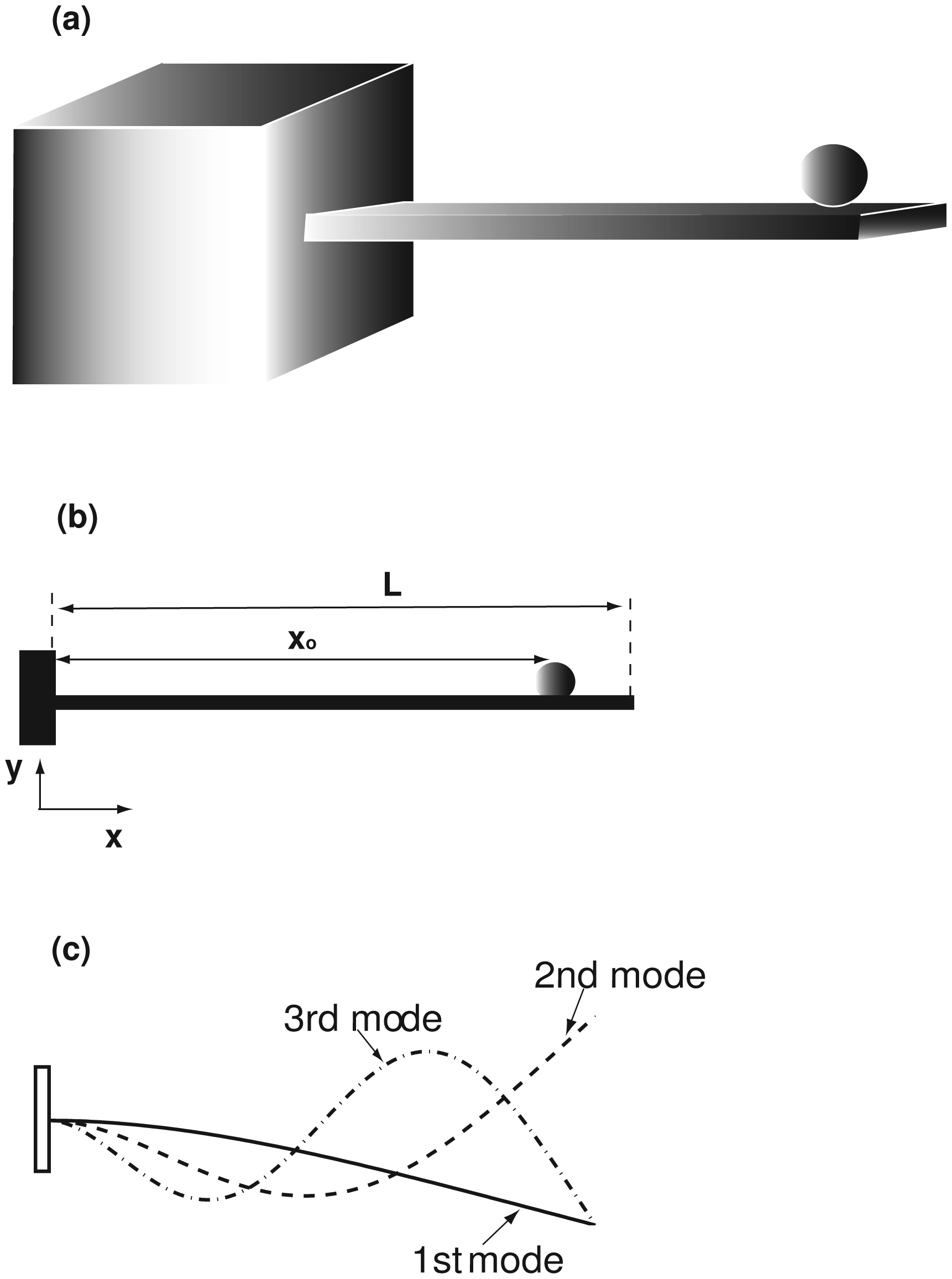
Figure 1a is a schematic of a cantilever beam with an accreted particle. A micro-/nano-mechanical resonator is often modeled as a beam structure [4,5,9,19,20]. For brevity, the beam governing equation is given as follows [22–24]:

$$[m+M_o{\delta }_D(x-x_o)]\frac{{\partial }^{2}w}{\partial t^2}+c\frac{\partial w}{\partial t}+EI\frac{{\partial }^{4}w}{\partial x^4}=0.$$

(1)

where m is the beam mass per unit length and m = ρbh (ρ, b and h are the mass density, width and thickness of the beam, respectively). M_o and x_o are the mass and position of an accreted particle, as shown in Figure 1b. δ_D is the Dirac delta function, which indicates that the accreted particle is modeled as a concentrated mass [22–24]. E, w and c are the beam Young's modulus, displacement and viscous damping, respectively. I is the moment of inertia and I = bh³/12 for a rectangular cross-section beam. There are two major assumptions in Equation (1): (1) the accreted particle only introduces the mass addition effect [25]; and (2) the application of the Dirac delta function assumes that the particle size is extremely small compared with that of the resonator. The accreted particles can change the resonator stiffness, which is mainly induced by two mechanisms: the stiffness of particles [26,27] and surface stress [28,29]. As the particle size is assumed very small, its stiffness can be ignored [26,27]. The presence of surface stress generates both the bending moment and axial force [29,30]; the axial force is responsible for the stiffness change. Surface stress is an important sensing mechanism for many receptor-based sensors [28,31], which is often induced by the receptor-ligand binding. The receptor-ligand binding is both highly sensitive and selective for the identification of an adsorbate/ligand [31]. However, it suffers from poor reproducibility, because of device-to-device variations in the coating. The challenges for developing robust and stable recognition methods through functionalized coatings (i.e., the receptor materials) and even interpreting the responses of receptor-based sensors still remain [31]. For a beam with a non-functionalized surfaces, surface stress is often very small and ignored. Because there is no stiffness change, the resonator described by Equation (1) is the so-called mass-loading sensor [25].

By introducing ξ = x/L$\tau =\sqrt{EI/m{L}^4}t$and W = w/L (L: beam length) [22,23], Equation (1) is nondimensionalized as follows:

$$[1+\alpha {\delta }_D(\xi -{\xi }_o)]\frac{{\partial }^{2}w}{\partial {\tau }^2}+C\frac{\partial w}{\partial \tau }+\frac{{\partial }^{4}W}{\partial {\xi }^4}=0.$$

(2)

where α and C are defined as follows:

$$\alpha =\frac{M_o}{mL},\hspace{1em}C=c\sqrt{\frac{L^4}{EIm}}$$

(3)

Physically, α is the ratio of the accreted mass to that of a uniform beam; C is the dimensionless damping. The Galerkin method is an efficient method for the eigenfrequency computation of a beam with small concentrated masses [22], which assumes the following form for W (ξ, τ):

$$W(\xi ,\tau )=\sum _{j=1}^N{a}_j(\tau ){\varphi }_j(\xi ),$$

(4)

where N is the mode number. φ_j(ξ) is the j -th mode of a uniform cantilever beam [32], and the first three are shown in Figure 1c; a_j(τ) is the unknown j-th modal amplitude with the presence of the concentrated mass [22]. Substitute Equation (4) into Equation (2), time φ_i(ξ) and integrate from 0 to 1; the following governing equations are derived:

$$\text{M}\ddot{\text{q}}+\text{D}\dot{\text{q}}+\text{Kq}=0.$$

(5)

Here, ${(}^{\cdot })=\frac{\partial }{\partial \tau }$and q is a vector given as q = (a₁,a₂, ….., a_N)^T . M, D and K are the N × N matrices of mass, damping and stiffness, respectively, which are given as the following by using the orthonormality property of φ_j(ξ) [22,23]:

$$\begin{array}{ccc}{\text{M}}_{\text{ij}}={\delta }_{\text{ij}}+\alpha {\varphi }_{\text{i}}\left({\xi }_o\right){\varphi }_{\text{j}}\left({\xi }_o\right),& {\text{D}}_{\text{ij}}=\text{C}{\delta }_{\text{ij}},& {\text{K}}_{\text{ij}}={\kappa }_{\text{j}}^4{\delta }_{\text{ij}}\end{array}.$$

(6)

where δ_ij is the Kronecker delta function; ${\kappa }_j^2$is the j-th (dimensionless) eigenfrequency of a uniform undamped beam, and the first three ${\kappa }_j^2$of a cantilever beam are given as follows [32]:

$$\begin{array}{ccc}{\kappa }_1^2={1.875}^2=3.516,& {\kappa }_2^2={4.694}^2=22.034,& {\kappa }_3^2={7.855}^2=61.697\end{array}.$$

(7)

Equation (5) is a damped nongyroscopic system and needs to be rewritten in the following form to formulate an eigenvalue problem [33]:

$$\text{M}\ast \dot{\text{x}}+\text{K}\ast \text{x}=0.$$

(8)

where x = (q̇, q) is a 2N vector; M^* and K^* are the 2N × 2N matrices defined as follows [33]:

$$\text{M}\ast =\left(\begin{array}{cc}\text{M}& 0\\ 0& -\text{K}\end{array}\right),\hspace{1em}\text{K}\ast =\left(\begin{array}{cc}\text{D}& \text{K}\\ \text{K}& 0\end{array}\right)$$

(9)

By letting x(τ)= e^iωτX, Equation (8) formulates a standard eigenvalue problem of AX = iωX with A = − (M^*)⁻¹K^* [33]. For Equation (8) to work, α and ξ_o must be supplied. Solving the eigenvalue problem of Equation (8) is not an easy task. As far as the concentrated mass is not located at the fixed end or node (i.e., φ_j(ξ_o) = 0), there are off-diagonal elements, and obtaining the analytical solution to Equation (8) is extremely difficult, if not impossible. With the presence of damping, the eigenvalue of ω is a complex variable of ω = R + iI. The real part (R) is the eigenfrequency, and the imaginary part (I) indicates the stability of the system [34]. Equation (8) yields 2N accurate eigenvalues of R and I.

If the concentrated mass is small, the following approximate analytical solution can be derived. By assuming $W={\sum }_{j=1}^N{b}_j{e}^{i\omega \tau }(\tau ){\varphi }_j(\xi )(\omega =R+iI)$and repeating the same procedure of the Galerkin method above, the following equation is derived:

$$\text{GB}=0.$$

(10)

where B = (b₁,b₂, ….b_N)^T and ${\text{G}}_{\text{ij}}={\text{G}}_{\text{ij}}^{\text{r}}+i{\text{G}}_{\text{ij}}^{\text{i}}$with ${\text{G}}_{\text{ij}}^{\text{r}}={\kappa }_j^4{\delta }_{ij}-IC{\delta }_{ij}-(R^2-I^2)-\left[{\delta }_{ij}+\alpha {\varphi }_i({\xi }_o){\varphi }_j({\xi }_o)\right]$and ${\text{G}}_{\text{ij}}^i=RC{\delta }_{ij}-2RI\left[{\delta }_{ij}+\alpha {\varphi }_i({\xi }_o){\varphi }_j({\xi }_o)\right]$. To have a nontrivial solution of B, the determinants of both the real part ${\text{G}}_{\text{ij}}^{\text{r}}$and imaginary part ${\text{G}}_{\text{ij}}^{\text{i}}$must be zero. Therefore, $\text{det}({\text{G}}_{\text{ij}}^{\text{r}})=0$and $\text{det}({\text{G}}_{\text{ij}}^{\text{i}})=0$formulate the eigenvalue problem for R and I, which can only be solved numerically. If the effect of off-diagonal elements are ignored, R and I are analytically obtained as follows by setting each diagonal element to zero:

$$R_j=\sqrt{\frac{{\kappa }_j^4}{1+\alpha {\varphi }_j^2({\xi }_o)}-\frac{C^2}{4{[1+\alpha {\varphi }_j^2({\xi }_o)]}^2},}$$

(11)

$$I_j=\frac{C}{2[1+\alpha {\varphi }_j^2({\xi }_o)]}.$$

(12)

$R_j={\kappa }_j^2$recovers the j-th eigenfrequency of a uniform undamped beam when α =0 and C =0 [22]. It is noteworthy to point out that when C = 0, $R_j=\sqrt{{\kappa }_j^4/[1+\alpha {\varphi }_j^2({\xi }_o)]}$

is the same one obtained by the Rayleigh–Ritz method [21]; R₁ also recovers the one obtained by using the curve fitting method when ξ_o =1 (at which φ₁(1) = 2) [10].

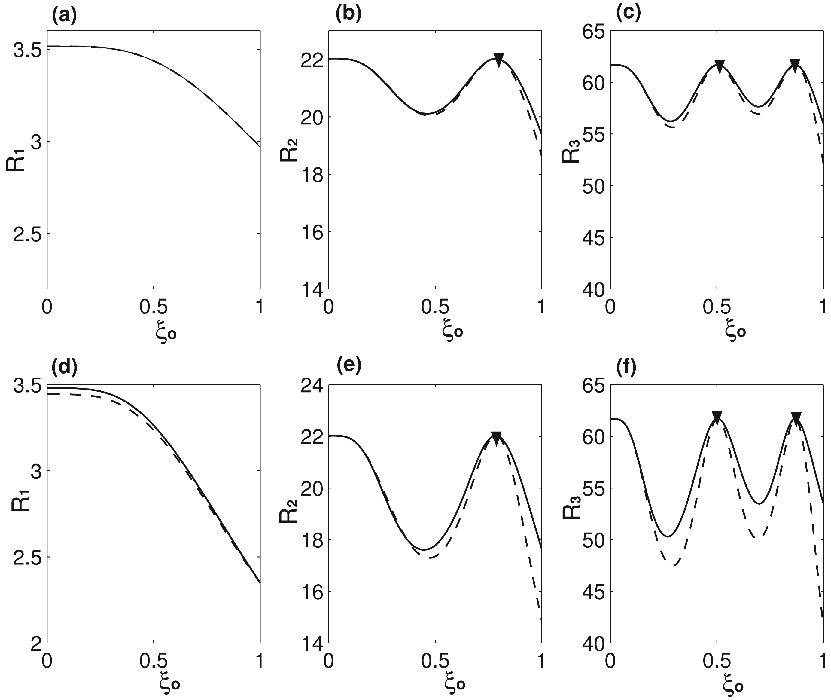
Figure 2 presents two case studies on the accuracy of Equation (11) as compared with Equation (8) for 0 ≤ ξ_o ≤ 1. Clearly, Equation (11) approximates much better for the case of α = 0.1 and C = 0.1, than that of α = 0.3 and C = 1. The reason is simple: Equation (11) ignores the off-diagonal elements, which become more important as α increases. The higher mode has higher mass sensitivity, because the effective mass of α is larger for higher modes [13], which is also the reason causing the larger error of Equation (11) for higher modes. As noticed in Figure 2, there is no error when a concentrated mass is placed at the node(s). There is no node for the first mode φ₁; ξ_nd = 0.782 is the node of the second mode φ₂; ξ_nd = 0.504 and ξ_nd =0.867 are the two nodes of the third mode φ₃. Mathematically, there are no off-diagonal elements, because φ_i(ξ_nd)=0 (i ≥ 2), and physically the effective mass of α becomes zero at node(s), which thus has no impact on the eigenfrequency of the corresponding mode.

From Equation (11), we have:

$$\alpha {\varphi }_j^2({\xi }_o)=\frac{{\kappa }_j^4+\sqrt{{\kappa }_j^8-R_j^2{C}^2}-2R_j^2}{2R_j^2}.$$

(13)

Actually, there are two solutions for $\alpha {\varphi }_j^2$

As for mass accretion on a mass resonator, $\alpha {\varphi }_j^2$is positive, as given in the above equation. The other solution of negative $\alpha {\varphi }_j^2$physically corresponds to a crack formation [34,35] or a vacancy defect [36], which is thus discarded. By setting j =1, 2 and 3 and from Equation (13), we have the following:

$$\frac{{\varphi }_2^2}{{\varphi }_1^2}({\xi }_o)={\left(\frac{R_1}{R_2}\right)}^2\frac{{\kappa }_2^4+\sqrt{{\kappa }_2^8-R_2^2{C}^2}-2R_2^2}{{\kappa }_1^4+\sqrt{{\kappa }_1^8-R_1^2{C}^2}-2R_1^2},$$

(14)

$$\frac{{\varphi }_3^2}{{\varphi }_1^2}({\xi }_o)={\left(\frac{R_1}{R_3}\right)}^2\frac{{\kappa }_3^4+\sqrt{{\kappa }_3^8-R_3^2{C}^2}-2R_3^2}{{\kappa }_1^4+\sqrt{{\kappa }_1^8-R_1^2{C}^2}-2R_1^2}.$$

(15)

For the convenience of statement, we define left-side functions of the Equations (14) and (15) as $F_{21}\left({\xi }_o\right)={\varphi }_2^2/{\varphi }_1^2\left({\xi }_o\right)$ and $F_{31}\left({\xi }_o\right)={\varphi }_3^2/{\varphi }_1^2\left({\xi }_o\right)$ ; right-side functions as $S_{21}\left(R_1,R_2\right)={\left(R_1/R_2\right)}^2\left({\kappa }_2^4+\sqrt{k_2^8-2R_2^2{C}^2}-2R_2^2\right)/\left({\kappa }_1^4+\sqrt{k_1^8-2R_1^2{C}^2}-2R_1^2\right)$ and $S_{31}\left(R_1,R_3\right)={\left(R_1/R_3\right)}^2\left({\kappa }_3^4+\sqrt{k_3^8-2R_3^2{C}^2}-2R_3^2\right)/\left({\kappa }_1^4+\sqrt{k_1^8-2R_1^2{C}^2}-2R_1^2\right)$ . One outstanding feature of Equations (14) and (15) is that α does not explicitly appear, whose information is contained in R₁, R₂, R₃. S₂₁ and S₃₁ are constants for given R₁, R₂, R₃. φ₁, φ₂ and φ₃ are the given functions of the first, second and third modes of a uniform undamped cantilever beam [32], respectively; the only variable in F₂₁ and F₃₁ is ξ_o.

3. Results and Discussion

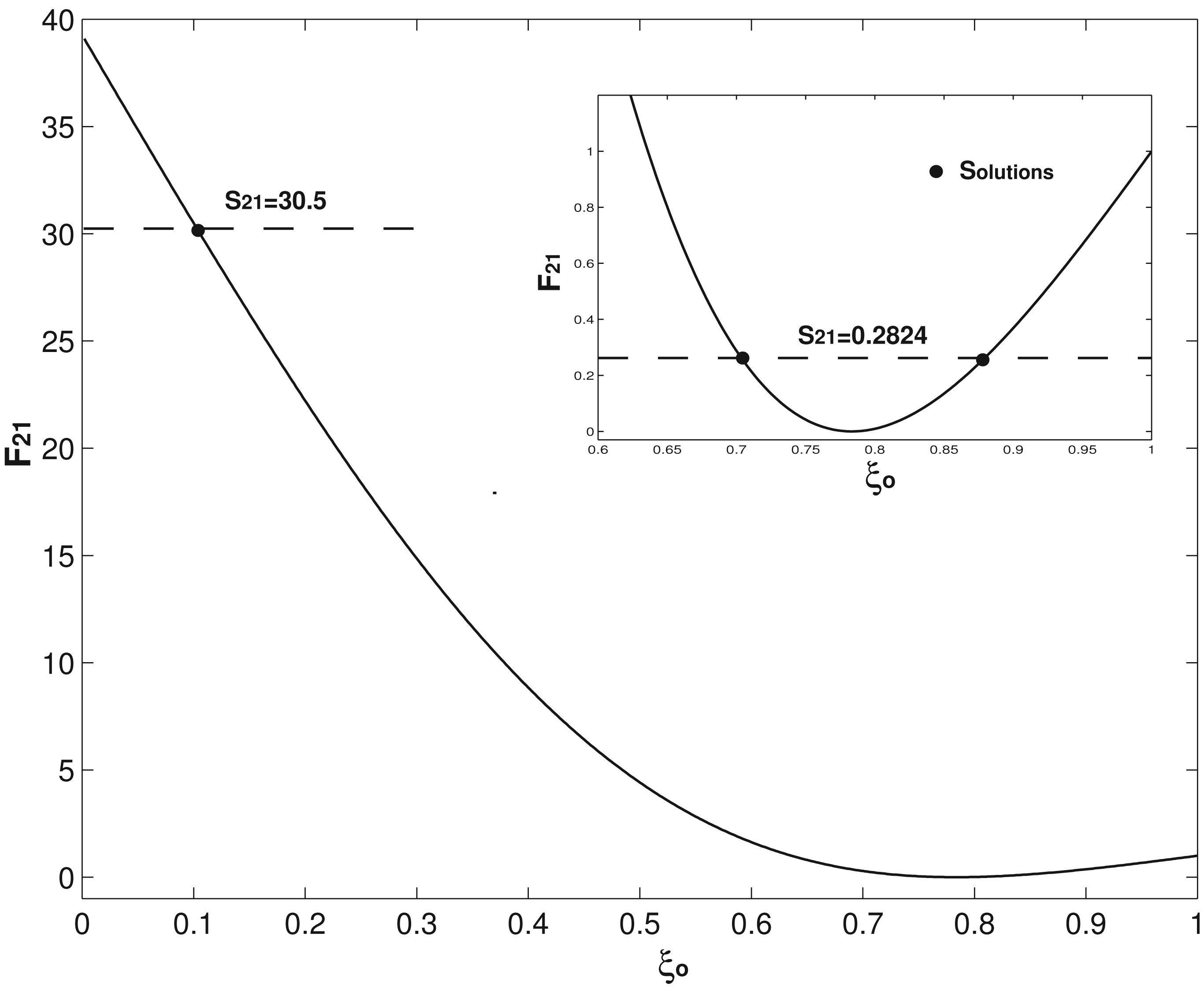
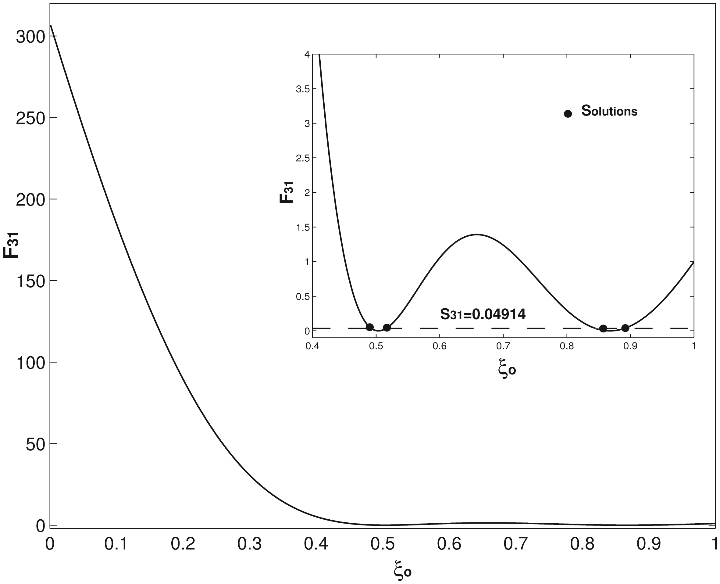
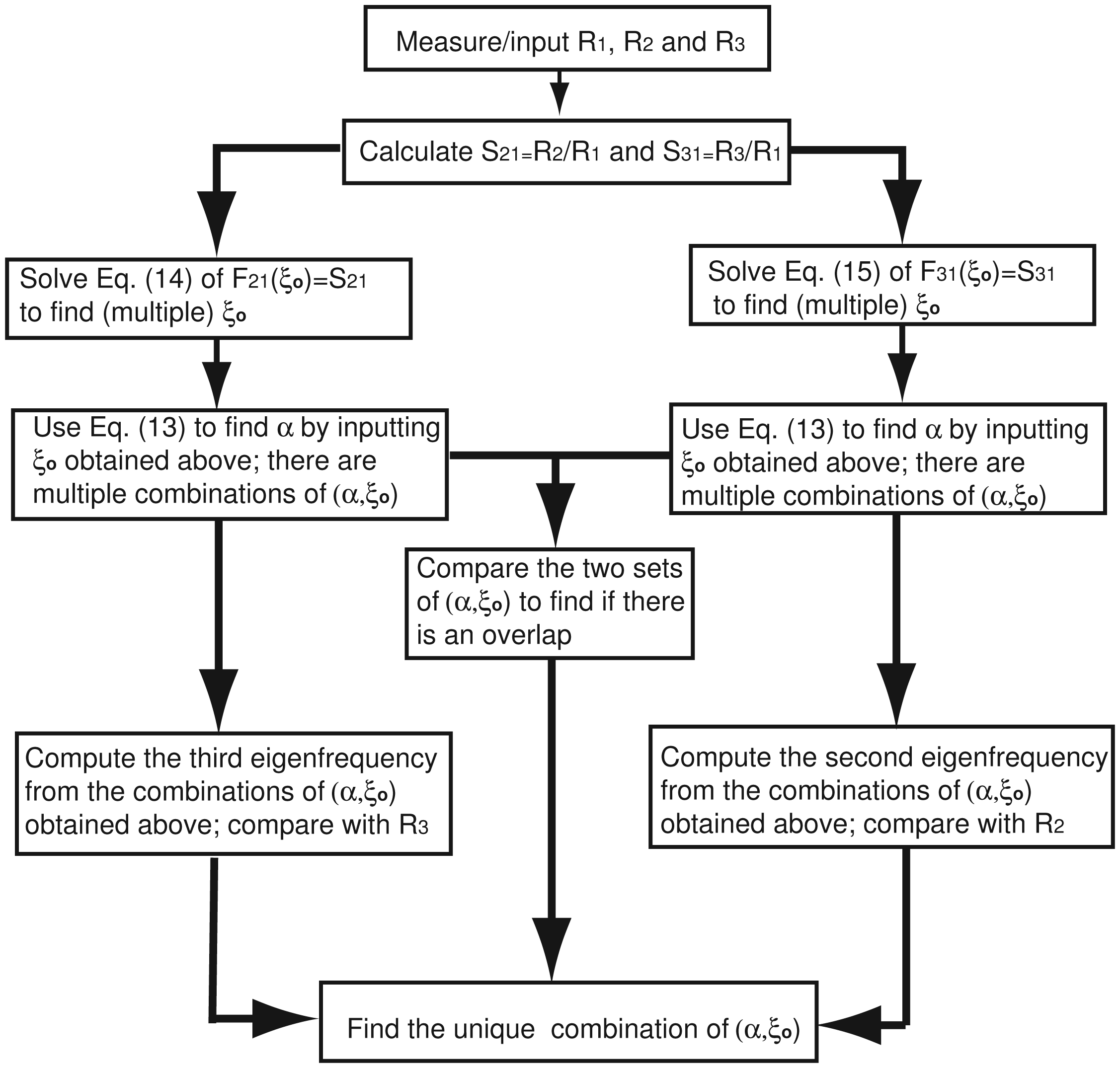
Two examples on how to use Equations (14) and (15) to determine the concentrate mass position and then use Equation (13) to find the corresponding mass are presented. For the first example of (α, ξ_o) = (0.1, 0.9) and C = 0.1, the first three eigenfrequencies are computed as R₁ =3.086, R₂ = 21.162 and R₃ = 61.25 by using Equation (8). Compared with those of a uniform undamped cantilever presented in Equation (7), all of these three eigenfrequencies decreases because of the concentrated mass and damping. In the application of a mass resonator, α and ξ_o are the two unknown parameters to be determined; R₁, R₂, R₃ are obtained by the experimental measurement. Now, suppose the above three R_is computed by Equation (8) are the experimentally obtained values, which give S₂₁ = 0.2824 and S₃₁ =0.04914. Equation (14) is first used, i.e., F₂₁(ξ_o)= S₂₁ =0.2824. Equation (14) is nonlinear, and the Newton–Rhapson method is required to solve ξ_o. Figure 3 presents the F₂₁ – ξ_o relation. As seen in the inset of Figure 3, there are two solutions in 0.636 ≤ ξ_o ≤ 1 and only one solution for ξ_o < 0.636, which physically means that if a concentrated mass locates at any place of ξ_o < 0.636 (or say S₂₁ > 1), its position can be uniquely determined by Equation (14). ξ_o of F₂₁(ξ_o) = 0.2824 is solved as ξ_o1 = 0.701 and ξ_o2 =0.884; substitute these two ξ_os values into Equation (13), and two corresponding α₁ = 0.213 and α₂ = 0.105 are obtained. Now, we have two possible combinations of (α, ξ_o) = (0.213, 0.701) and (0.105, 0.884). Physically, these two combinations generate the same first and second eigenfrequencies, which is the typical scenario encountered in solving an inverse problem [27,29]. To tell which one is the correct one, F₃₁(ξ_o)= S₃₁ =0.04914 is needed, which gives four solutions of ξ_o1 = 0.4903, ξ_o2 = 0.5182, ξ_o3 = 0.8409 and ξ_o4 = 0.8949. Again, substitute these four ξ_os into Equation (13) and four corresponding αs are obtained as: α₁ = 0.692, α₂ = 0.5727, α₃ = 0.1222 and α₄ = 0.102. There are four combinations, (α, ξ_o) = (0.692, 0.4903), (0.5727, 0.5182), (0.1222, 0.8409) and (0.102, 0.8949), and physically, these four combinations generate the same first and third eigenfrequencies. As seen in Figure 4, there are four solutions in 0.451 ≤ ξ_o ≤ 1, and only one in ξ_o < 0.451. Again, this means that if a concentrated mass locates at any place of ξ_o < 0.451 (or say S₃₁ > 1), its position can be uniquely determined by Equation (15). Now, compare the two combinations obtained by Equation (14) and four combinations obtained by Equation (15); it is not hard to conclude that the only overlapped combination is (α, ξ_o)= (0.105, 0.884)/(0.102, 0.8949). Here, the (small) difference between these two combinations is caused by our approximate analytical expression having different errors on different modes, as analyzed above. However, it is still good enough for us to tell which two combinations overlap. Compared with the actual combination of (0.1, 0.9), the accuracy of our method is demonstrated. Alternatively, instead of using $F_{\text{31}}\left({\xi }_o\right)=S_{\text{31}},F_{\text{32}}\left({\xi }_o\right)={\varphi }_3^2/{\varphi }_2^2\left({\xi }_o\right)=S_{\text{32}}$ can also be used to determine (α, ξ_o) together with F₂₁(ξ_o)= S₂₁. However, keep in mind that F₃₂ becomes infinite at ξ_nd = 0.782, which is the node of φ₂ and makes the numerical solution more difficult and less accurate. The first three eigenfrequencies of (0.1, 0.9), two combinations obtained by Equation (14) and four combinations obtained by Equation (15) are listed in

Table 1. The first three eigenfrequencies for different combinations of (α, ξ_o). The combinations are found by Equations (14) and (15), which use the information of two eigenfrequencies.

(α, ξo)/Ri	R1	R2	R3
(0.1, 0.9)	3.086	21.162	61.25
(0.213, 0.701)	3.084	21.334	54.9
(0.105, 0.884)	3.086	21.353	61.58
(0.692, 0.4903)	3.075	15.264	61.54
(0.5727, 0.5182)	3.077	16.142	61.52
(0.122, 0.8409)	3.085	21.78	61.36
(0.102, 0.8949)	3.085	21.22	61.37

. Mathematically, Equation (14) or Equation (15), which, in essence, only uses the information of two (measured) eigenfrequencies, cannot uniquely determine the actual combination of (α, ξ_o). Physically, Table 1 contains all of the possible combinations of (α, ξ_o) (six in total) determined by two eigenfrequencies; the actual combination of (α, ξ_o), which needs to satisfy all three (measured) eigenfrequencies, is among these six possible combinations. There is another effective way to determine the concentrated mass and its position. Equation (14) gives the two combinations with the same first and second eigenfrequencies. If the third eigenfrequency is computed, as seen in Table 1, R₃ = 54.9 for (0.213, 0.701), which deviates significantly from the input/measured value of 61.25 and is thus excluded. The above solution procedure can be summarized by the following flow chart (Figure 5). Measuring the mode shapes, which is frequently done in the structural damage identification [35], can also be used to determine the combination. Although Equation (14) gives two combinations with the same first and second eigenfrequencies, their corresponding mode shapes are different, and mode shape comparison can thus help to determine the right combination. However, the method of the mode shape comparison can be very difficult, especially when the concentrated mass is very small.

In the above example, the concentrated mass of α = 0.1 and damping C = 0.1 (corresponding to a quality factor of Q ≈ 35) are both relatively large. As demonstrated in the next example, our method achieves a much better accuracy for smaller α and C, which is the case in many mass resonator applications [9,10,13,16]. Because the eigenfrequency of a beam is proportional to $\sqrt{EI/(m{L}^4)}=h/L^2\sqrt{E/\rho }$ [23], there are two major methods to enhance the mass resonator sensitivity: (1) to scale down the resonator size [8,16,26] to achieve a larger h/L²; and (2) to use the materials with large E/ρ, such as graphene [12] and carbon nanotube [9,20]. Both methods result in increasing eigenfrequencies. With a large eigenfrequency, a tiny fractional change in eigenfrequency is still absolutely large enough to be detected [6], and the sensitivity is thus enhanced.

For comparison reasons, the characteristics of Dohn's method [21] is summarized as follows: (1) the damping effect is not included; (2) (at least) four eigenfrequencies are needed to determine the concentrated mass and position; (3) a robust and complex fitting procedure is needed; and (4) more importantly, their method has “inherent shortcomings”, which cannot correctly determine the mass position when ξ_o < 0.2 or α < 0.0084 [37]. The second example is presented to show that our method further stands out in the application scenario of ξ_o close to the fixed end with smaller α and C. (α, ξ_o) = (0.0084, 0.1) and C =0 [21] are taken and R₁ =3.516 and R₂ = 22.034 are computed by Equation (8), which as inputs give S₂₁ = 30.5. By using Equation (14), ξ_o = 0.1 is uniquely determined as presented in Figure 3; then substitute this ξ_o = 0.1 value into Equation (13), α = 0.0084 is obtained. Now, this method obtains the exact combination of (0.0084, 0.1) and only requires the measurements/inputs of two eigenfrequencies.

In a real application, a micro-/nano-mechanical resonator can be cleaned by passing a large electric current, which generates Joule heating and thus boils off the adsorbates [20]. However, it is (almost) impossible to control the adsorption process to realize the scenario of just one adsorbate. As the model and method are developed for the one particle case, we have to address how the inverse problem solving method can be applied to the general scenario of multiple accreted particles. Theoretically, when the particle number N ≥ 2, we can still repeat the above solving procedures with the measurement of up to 3N resonant frequencies. However, if N is large, the method becomes more complex and much less efficient. Furthermore, experimentally measuring a large number of resonant frequencies is also a big problem, especially for those (very) high modes. Fortunately, we can avoid solving the problem of multiple particles. The reasons are the following three. Firstly, the current state-of-the-art micro-/nano-mechanical resonators are very sensitive, which can detect the shifts of resonant frequencies induced by a single adsorption event. The step-wise decrease of resonant frequency recorded in the experiments indicates the discrete nature of adsorbates arriving at the micro-/nano-mechanical resonator one by one, which is also the hallmark of sensing the individual adsorption events of one protein [4,5], one atom [9,19] and one molecule [20]. By building the histogram of count versus frequency shift for the ensemble of sequential single gold atom adsorption, Jensen et al. [19] were able to identify with a certain confidence level that the gold atomic mass ranges between 0.1 zg and 1 zg, as compared with the true value of 0.327 zg (1 zg = 10⁻²¹ g). Proteins in solution often aggregate to form different oligomers, which have different masses [4]. By building the histograms of event probability versus frequency shift for the ensembles of sequential single protein adsorption, Naik et al. [4] achieved a marvelous result: from the data of 578 individual adsorption events, they can tell that the “nominally pure” protein of bovine serum albumin (BSA) consists of a monomer, dimer, trimer, tetramer, pentamer and their composition. With the help of the second resonant frequency, Hanay et al. [5] achieved an even more astonishing result: from the data of 74 individual adsorption events, they can identify 14 different isoforms and their composition of the human IgM antibody. Our inverse problem solving method can do similar work with one datum of one single adsorption event. The underlying rationale is that the above statistics methods [4,5,19] deal with two convolving parameters of an adsorbate: mass and position; therefore, they need tens or hundreds of data to “decouple” these two parameters by assuming certain distribution rules, such as Gaussian; because our method can determine the mass and position of an adsorbate, one adsorption event is enough. Secondly, we need the assumption that the mass of previously adsorbed particles is very small compared with that of a resonator. When there are multiple (unknown) adsorbates, α defined in Equation (3) becomes the following:

$$\alpha =\frac{M_o}{mL+{\sum }_i^N{M}_i}\approx \frac{M_o}{mL}$$

(16)

where N is the (unknown) number of adsorbates and M_i is the corresponding (unknown) mass; M_o is the mass of an incoming particle. The above approximation holds by assuming ${\sum }_i^N{M}_i\ll mL$. As discussed above, one great advantage of a micro-/nano-mechanical resonator sensor is to detect the tiny fractional shifts of resonant frequencies, and a very tiny amount of mass can thus be sensed. In Chiu's experiment [9], the mass of the carbon nanotube resonator is around 1000 zg; the adsorbates are the molecules of noble gas, and the atomic masses of xenon and argon are 0.218 zg and 0.066 zg, which corresponds to α =2.18 × 10⁻⁴ and α = 6.6 × 10⁻⁵, respectively. The mass of previously adsorbed particles has little or no impact on the resonant frequency; the mass and position of a landing adsorbate are mainly or solely responsible for the step-wise resonant frequency drop observed in the experiments, which is also the implicit assumption used in the above statistics methods [4,5,19]. Thirdly, the multiple resonant frequencies induced by an adsorbate can be measured (almost) simultaneously between two individual adsorption events [5]. The resonant frequency of a micro-/nano-mechanical resonator can be as high as one gigahertz or even higher [8,20], and the time required to measured the resonant frequencies is extremely small. On the other hand, the adsorption rate is relatively slow, for example, the argon adsorption rate is 0.09 atom per second [9]. In conjunction with these three conditions, our inverse problem solving method can determine the mass and position of a particle by one single adsorption event, which is more efficient than the statistics approaches [4,5,19]. Furthermore, the statistics approaches are complex, and histogram analysis is time-consuming, which hinders their application in real-time particle mass spectrometry [37]. On the other hand, solving Equations (14) and (15) is much simpler and straightforward, which is capable of real-time analysis.

4. Conclusions

An approximate analytical solution for the eigenfrequencies of a mass resonator with a cantilever structure is presented, and its accuracy for small concentrated mass and damping is also demonstrated. The approximate analytical solution is obtained by ignoring the off-diagonal elements of the mass matrix formed by the Galerkin method. The error of the approximate analytical solution becomes large when the concentrated mass or damping is large. The approximate analytical solution can be used to uniquely determine one concentrated mass and its position by measuring at most the first three eigenfrequencies (sometimes only two). The possibility of applying the method to the practical application of the micro-/nano-mechanical resonator mass sensing is discussed. The method can be easily extended to the resonator with the clamped-clamped boundary conditions [8,16,20] by simply changing the mode shape function of φ_i.

References

- Aebersold, R.; Mann, M. Mass spectrometry-based proteomics. Nature 2003, 422, 198–207. [Google Scholar]
- Domon, B.; Aebersold, R. Mass spectrometry and protein. Science 2006, 312, 212–216. [Google Scholar]
- Gil-Santos, E.; Ramos, D.; Martinez, J.; Fernandez-Regulez, M.; Garcia, R.; San Paulo, A.; Calleja, M.; Tamayo, J. Nanomechanical mass sensing and stiffness spectrometry based two-dimensional vibrations of resonant nanowires with yoctogram resolution. Nat. Nanotech. 2010, 5, 641–645. [Google Scholar]
- Naik, A.K.; Hanay, M.S.; Hiebert, W.K.; Feng, X.L.; Roukes, M.L. Towards single-molecule nanomechanical mass spectrometry. Nat. Nanotech. 2009, 4, 445–450. [Google Scholar]
- Hanay, M.S.; Kelber, S.; Naik, A.K.; Chi, D.; Hentz, S.; Bullard, E.C.; Colinet, E.; Duraffourg, L.; Roukes, M.L. Single-protein nanomechanical mass spectrometry in real time. Nat. Nanotech. 2012, 7, 602–608. [Google Scholar]
- Knobel, R.G. Weighing single atoms with a nanotube. Nat. Nanotech. 2008, 3, 525–526. [Google Scholar]
- Hiebert, W. Devices reach single-proton limit. Nat. Nanotech. 2012, 7, 278–280. [Google Scholar]
- Huang, X.; Zorman, C.A.; Mehregany, M.; Roukes, M.L. Nanoelectromechanical systems: Nanodevice motion at microwave frequencies. Nature 2003, 421. [Google Scholar] [CrossRef]
- Chiu, H.; Hung, P.; Postma, H.; Bockrath, M. Atomic-scale mass sensing using carbon nanotube resonators. Nano Lett. 2008, 8, 4342–4346. [Google Scholar]
- Ilic, B.; Craighead, H.G.; Krylov, S.; Senaratne, W.; Ober, C.; Neuzil, P. Attogram detection using nanoelectromechanical oscillators. J. Appl. Phys. 2004, 95, 3694–3703. [Google Scholar]
- Burg, T.P.; Manalis, S.R. Suspended microchannel resonators for biomolecular detection. Appl. Phys. Lett. 2003, 83, 2698–2700. [Google Scholar]
- Bunch, J.S.; van der Zande, A.M.; Verbridge, S.S.; Frank, I.W.; Tanenbaum, D.M.; Parpia, J.M.; Craighead, H.G.; McEuen, P.L. Electromechanical resonators from graphene sheets. Science 2007, 315, 490–493. [Google Scholar]
- Dohn, S.; Sandberg, R.; Svendsen, W.; Boisen, A. Enhanced functionality of cantilever based mass sensors using higher modes. Appl. Phys. Lett. 2005, 86. [Google Scholar] [CrossRef]
- Yu, H.; Li, X.X. Bianalyte mass detection with a single resonant microcantilever. Appl. Phys. Lett. 2009, 94. [Google Scholar] [CrossRef]
- Burg, T.P.; Godin, M.; Knudsen, S.M.; Shen, W.; Carlson, G.; Foster, J.S.; Babcock, K.; Manalis, S.R. Weighing of biomolecules, single cells and single nanoparticles in fluid. Nature 2007, 446, 1066–1069. [Google Scholar]
- Ekinci, K.L.; Yang, Y.T.; Roukes, M.L. Ultimate limits to inertial mass sensing based upon nanoelectromechanical systems. J. Appl. Phys. 2004, 95, 2682–2689. [Google Scholar]
- Grover, W.H.; Bryan, A.K.; Diez-Silva, M.; Suresh, S.; Higgins, J.M.; Manalis, S.R. Measuring single-cell density. Proc. Natl. Acad. Sci. USA. 2011, 108, 10992–10996. [Google Scholar]
- Gupta, A.; Akin, D.; Bashir, R. Single virus particle mass detection using microresonator with nanoscale thickness. Appl. Phys. Lett. 2004, 84, 1976–1978. [Google Scholar]
- Jensen, K.; Kim, K.; Zettl, A. An atomic-resolution nanomechanical mass sensor. Nat. Nanotech. 2008, 3, 533–537. [Google Scholar]
- Chaste, J.; Eichler, A.; Moser, J.; Ceballos, G.; Rurali, R.; Bachtold, A. A nanomechanical mass sensor with yoctogram resolution. Nat. Nanotech. 2012, 7, 301–304. [Google Scholar]
- Dohn, S.; Svendsen, W.; Boisen, A.; Hansen, O. Mass and position determination of attached particles on cantilever based mass sensors. Rev. Sci. Instrum. 2007, 78. [Google Scholar] [CrossRef]
- Zhang, Y. Eigenfrequency Computation of beam/plate carrying concentrated mass/spring. J. Vibr. Acoust. 2011, 133. [Google Scholar] [CrossRef]
- Zhang, Y.; Murphy, K.D. Multi-modal analysis on the intermittent contact dynamics of atomic force microscope. J. Sound Vib. 2011, 330, 5569–5582. [Google Scholar]
- Li, H.; Chen, Y.; Dai, L. Concentrated-mass cantilever enhances multiple harmonics in tapping-mode atomic force microscopy. Appl. Phys. Lett. 2008, 92. [Google Scholar] [CrossRef]
- Chen, D.; Wang, J.; Xu, Y.; Li, D.; Zhang, L.; Li, Z. Highly sensitive detection of organophosphorus pesticides by acetylcholinesterase-coated thin film bulk acoustic resonator mass-loading sensor. Biosens. Bioelectron. 2013, 41, 163–167. [Google Scholar]
- Ramos, D.; Tamayo, J.; Mertens, J.; Calleja, M.; Zaballos, A. Origin of the response of nanomechanical resonators to bacteria adsorption. J. Appl. Phys. 2006, 100. [Google Scholar] [CrossRef]
- Zhang, Y. Detecting the stiffness and mass of biochemical adsorbates by a resonator sensor. Sens. Actuators B Chem. 2014, 202, 286–293. [Google Scholar]
- Ji, H.; Thundat, T. In situ detection of calcium ions with chemically modified microcantilever. Biosens. Bioelectron 2002, 17, 337–343. [Google Scholar]
- Zhang, Y. Determining the adsorption-induced surface stress and mass by measuring the shifts of resonant frequencies. Sens. Actuators A Phys. 2013, 194, 169–175. [Google Scholar]
- Finot, E.; Passian, A.; Thundat, T. Measurement of mechanical properties of cantilever shaped materials. Sensors 2008, 8, 3497–3541. [Google Scholar]
- Farahi, R.H.; Passian, A.; Tetard, L.; Thundat, T. Critical issues in sensor science to aid food and water safety. ACS Nano. 2012, 6, 4548–4556. [Google Scholar]
- Chang, T.C.; Craig, R.R. Normal modes of uniform beams. J. Engr. Mech. 1969, 195, 1027–1031. [Google Scholar]
- Meirovitch, L. Computational Methods in Structural Dynamics; Sijthoff & Noordhoff Inc.: Rockville, MD, USA; ,1980. [Google Scholar]
- Murphy, K.D.; Zhang, Y. Vibration and stability of a cracked translating beam. J. Sound Vib. 2000, 237, 319–335. [Google Scholar]
- Ge, M.; Lui, E.M. Structural damage identification using system dynamic properties. Comput. Struct. 2005, 83, 2185–2196. [Google Scholar]
- Panchal, M.B.; Upadhyay, S.H.; Harsha, S.P. Vibrational characteristics of defective single walled BN nanotube based nanomechanical mass sensors: single atom vacancies and divacancies. Sens. Actuators A Phys. 2013, 197, 111–121. [Google Scholar]
- Schmid, S.; Dohn, S.; Boisen, A. Real-time mass spectrometry based on resonant micro strings. Sensors 2010, 10, 8092–8100. [Google Scholar]