
PRIMAL: Page Rank-Based Indoor Mapping and Localization Using Gene-Sequenced Unlabeled WLAN Received Signal Strength

Abstract
:1. Introduction
2. Related Work

| Symbols | Description |
|---|---|
| Time duration of the event z | |
| The i-th RSS vector in sequence a | |
| The j-th RSS vector in sequence b | |
| Matching score between and | |
| m | Length of sequence a |
| n | Length of sequence b |
| Similarity function of RSS pair and | |
| Gap scoring function with depth k | |
| The l-th RSS sequence | |
| The i-th RSS vector in |
3. System Description
3.1. Construction of the Mobility Graph


3.2. Construction of the Signal Graph
3.2.1. RSS Characteristics

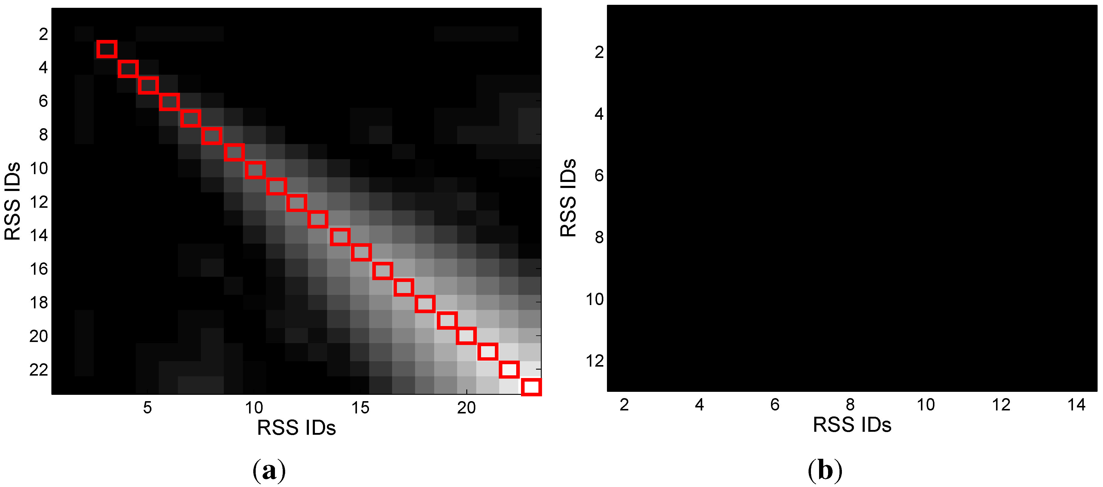
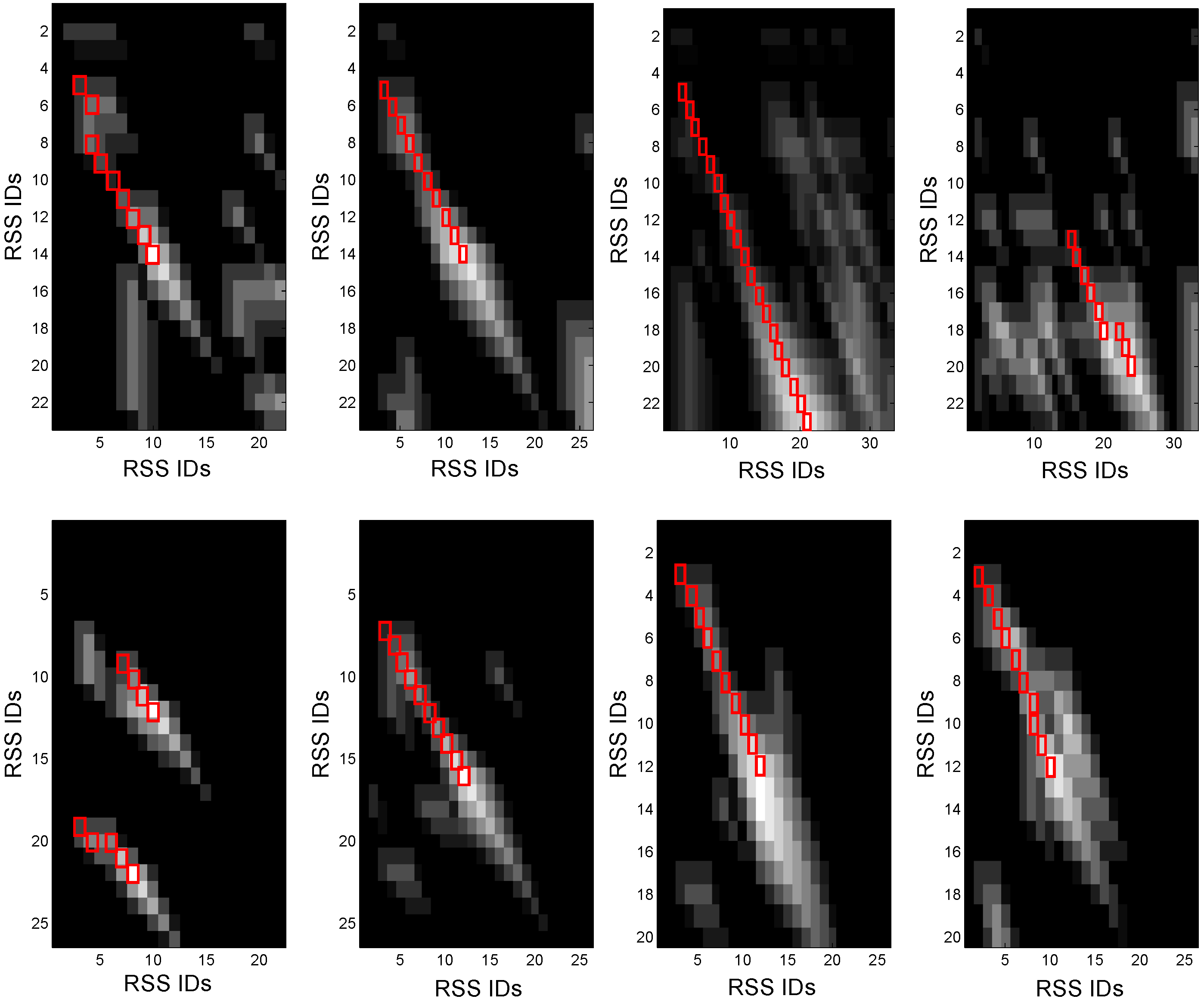
3.2.2. Gene Sequencing


| Traces | Number of Collected RSS Sequences |
|---|---|
| Lobby 2 → Lobby 1 | 10 |
| Lobby 2 → Corridor 2 | 5 |
| Corridor 2 → Lobby 1 | 7 |
| Lobby 1 → Corridor 2 → Lobby 3 | 2 |
| Corridor 3 → Corridor 2 | 9 |
| Lobby 1 → Lobby 2 | 19 |
| Corridor 2 → Corridor 3 | 4 |
| Lobby 2 → Corridor 3 | 1 |
| Lobby 1 → Corridor 2 → Corridor 1 | 8 |
| Lobby 1 → Corridor 3 | 3 |
| Corridor 2 → Lobby 2 | 2 |
| Corridor 3 → Lobby 1 | 2 |
| Lobby 2 → Corridor 2 → Corridor 1 | 5 |
| Lobby 1 → Corridor 2 | 8 |
| Corridor 1 → Corridor 2 → Lobby 1 | 3 |
| Corridor 3 → Lobby 2 | 2 |
| Corridor 1 → Corridor 2 → Lobby 2 | 4 |
- as and
- as and
- as and
- as and
- as and
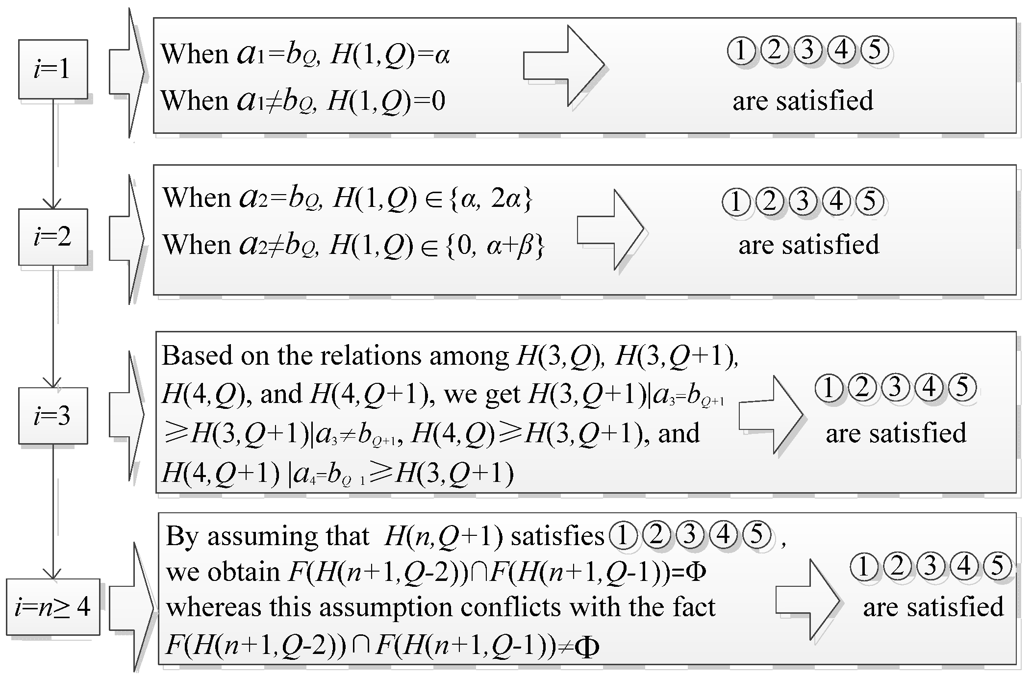
- (i)
- If the current RSS vector is matched with an RSS vector, but mismatched with the next one, the matching score of the current RSS pair is not lower than the one of the next pair;
- (ii)
- if the current RSS pair is matched, whereas the next RSS pair is mismatched, the matching score of the current RSS pair is not lower than the one of the next pair;
- (iii)
- if the current RSS pair is matched, while the next RSS pair is also matched, the matching score of the current RSS pair is not higher than the one of the next pair;
- (iv)
- if the current RSS vector is mismatched and still mismatched with the next one, the matching score of the current RSS pair is not lower than the one of the next pair;
- (v)
- if the current RSS pair is mismatched, whereas the next RSS pair is matched, the matching score of the current RSS pair is not higher than the one of the next pair.


3.3. Graph Exhibition by Graph Drawing

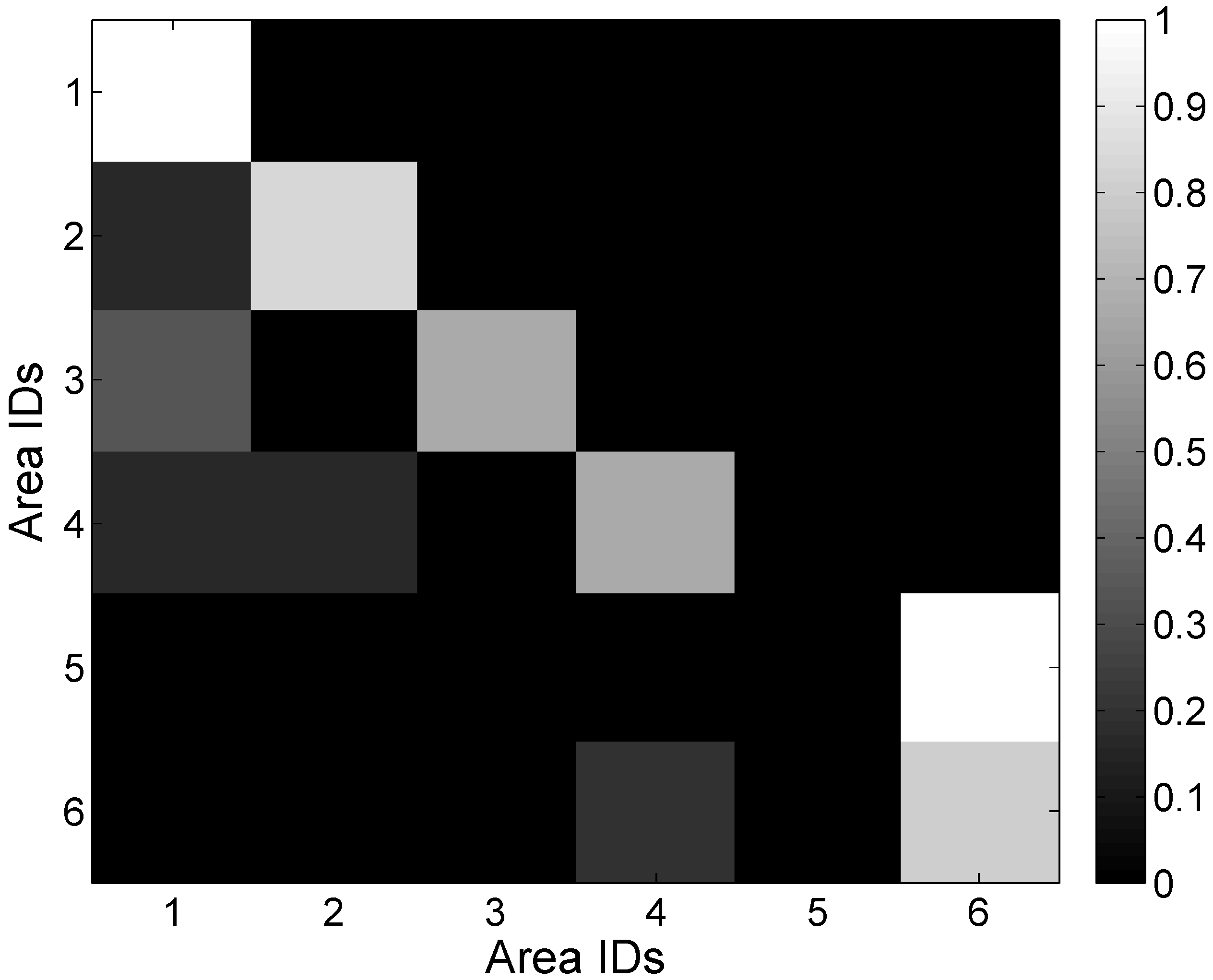
3.4. Page Rank Algorithm

| IDs in MG | 1 | 2 | 3 | 4 | 5 | 6 | |
|---|---|---|---|---|---|---|---|
| Probabilities | 0.27 | 0.11 | 0.05 | 0.22 | 0.03 | 0.09 | |
| IDs in SG | 1 | 2 | 3 | 4 | 5 | 6 | 7 |
| Probabilities | 0.19 | 0.03 | 0.026 | 0.03 | 0.026 | 0.01 | 0.02 |
| IDs in SG | 8 | 9 | 10 | 11 | 12 | 13 | 14 |
| Probabilities | 0.02 | 0.02 | 0.01 | 0.02 | 0.01 | 0.02 | 0.02 |
| IDs in SG | 15 | 16 | 17 | 18 | 19 | ||
| Probabilities | 0.01 | 0.02 | 0.01 | 0.02 | 0.01 |

3.5. Target Localization
4. Performance Evaluation
4.1. Localization Accuracy


4.2. Parameter Discussion


5. Conclusions and Future Work
Supplementary Materials
Acknowledgments
Author Contributions
Conflicts of Interest
Appendix
Proof of the Scoring Function

References
- Pei, L.; Chen, R.; Liu, J.; Kuusniemi, H. Using inquiry-based bluetooth rssi probability distributions for indoor positioning. J. Glob. Position. Syst. 2010, 9, 122–130. [Google Scholar]
- Kim, S.J.; Kim, B.K. Dynamic ultrasonic hybrid localization system for indoor mobile robots. IEEE Trans. Ind. Electron. 2013, 60, 4562–4573. [Google Scholar] [CrossRef]
- Chang, S.R.; Lin, W.; Chang, S.; Tu, C.; Wei, C.; Chien, C.; Tsai, C.; Chen, J.; Chen, A. A dual-band RF transceiver for multistandard WLAN applications. IEEE Trans. Microw. Theory Tech. 2005, 53, 1048–1055. [Google Scholar] [CrossRef]
- Lai, M.; Jeng, S. A microstrip three-port and four-channel multiplexer for WLAN and UWB coexistence. IEEE Trans. Microw. Theory Tech. 2005, 53, 3244–3250. [Google Scholar] [CrossRef]
- Yang, S.; Jung, E.; Han, S.K. Indoor location estimation based on LED visible light communication using multiple optical receivers. IEEE Commun. Lett. 2013, 17, 1834–1837. [Google Scholar] [CrossRef]
- Liu, M.; Qiu, K.; Che, S.; Li, S.; Hussain, B.; Wu, L.; Yue, C. Towards indoor localization using visible light Communication for consumer electronic devices. In Proceedings of the IEEE/RSJ International Conference in Intelligent Robots and Systems, Chicago, IL, USA, 14–18 September 2014; pp. 143–148.
- Vegni, A.M.; Biagi, M. An indoor localization algorithm in a small-cell LED-based lighting system. In Proceedings of the International Conference on Indoor Positioning and Indoor Navigation, Sydney, NSW, Australia, 13–15 November 2012; Volume 147, pp. 1–7.
- Ma, L.; Xu, Y. Received Signal Strength Recovery in Green WLAN Indoor Positioning System Using Singular Value Thresholding. Sensors 2015, 15, 1292–1311. [Google Scholar] [CrossRef] [PubMed]
- Du, Y.; Yang, D.; Xiu, C. Novel Method for Constructing a WIFI Positioning System with Efficient Manpower. Sensors 2015, 15, 8358–8381. [Google Scholar] [CrossRef] [PubMed]
- Sun, Y.; Xu, Y.; Li, C.; Ma, L. Kalman/Map filtering-aided fast normalized cross correlation-based Wi-Fi fingerprinting location sensing. Sensors 2013, 13, 15513–15531. [Google Scholar] [CrossRef] [PubMed]
- Zhou, M.; Wang, A.K.; Tian, Z.; Luo, X.; Xu, K.; Shi, R. Personal Mobility Map Construction for Crowd-Sourced Wi-Fi Based Indoor Mapping. IEEE Commun. Lett. 2014, 18, 1427–1430. [Google Scholar] [CrossRef]
- Chen, Y.; Fracisco, J.A.; Trappe, W.; Martin, R.P. A parctical approach to landmark deployment for indoor localization. In Proceedings of the 3rd Annual IEEE Communications Society on Sensor and Ad Hoc Communications and Networks, Reston, VA, USA, 28 September 2006; pp. 3429–3443.
- Zhou, M.; Wang, A.K.; Tian, Z.; Zhang, V.Y.; Yu, X.; Luo, X. Adaptive Mobility Mapping for People Tracking Using Unlabelled Wi-Fi Shotgun Reads. IEEE Commun. Lett. 2013, 17, 87–90. [Google Scholar] [CrossRef]
- Zhou, M.; Xu, Y.; Ma, L.; Tian, S. On the statistical errors of RADAR location sensor networks with built-in Wi-Fi Gaussian linear fingerprints. Sensors 2012, 12, 3605–3626. [Google Scholar] [CrossRef]
- Ma, L.; Xu, Y.; Wu, D. A novel two-step WLAN indoor positioning method. J. Comput. Inf. Syst. 2010, 6, 4627–4636. [Google Scholar]
- Wang, B.; Zhou, S.; Liu, W.; Mo, Y. Indoor localization based on curve fitting and location search using received signal strength. IEEE Trans. Ind. Electron. 2015, 62, 572–582. [Google Scholar] [CrossRef]
- Zhou, M.; Tian, Z.; Xu, K.; Yu, X.; Hong, X.; Wu, H. SCaNME: Location Tracking System in Large-Scale Campus Wi-Fi Environment Using Unlabeled Mobility Map. Expert Syst. Appl. 2014, 41, 3429–3443. [Google Scholar] [CrossRef]
- Bahl, P.; Padmanabhan, V.N. RADAR: An in-building RF-based user location and tracking system. In Proceedings of the IEEE INFOCOM, Tel Aviv, Israel, 26–30 March 2000; Volume 2, pp. 775–784.
- Youssef, M.; Agrawala, A. The Horus WLAN location determination system. In Proceedings of the 3rd International Conference on Mobile Systems, Applications, and Services, Seattle, WA, USA, 6–8 June 2005; pp. 205–218.
- Kaemarungsi, K.; Krishnamurthy, P. Analysis of WLAN’s received signal strength indication for indoor location fingerprinting. Pervasive Mob. Comput. 2012, 8, 292–316. [Google Scholar] [CrossRef]
- Zhou, M.; Tian, Z.; Xu, K.; Yu, X.; Wu, H. Theoretical Entropy Assessment of Fingerprint-based Wi-Fi Localization Accuracy. Expert Syst. Appl. 2013, 40, 6136–6149. [Google Scholar] [CrossRef]
- Wu, C.; Yang, Z.; Liu, Y.; Xi, W. WILL: Wireless indoor localization without site survey. IEEE Trans. Parallel Distrib. Syst. 2013, 24, 839–848. [Google Scholar]
- Shin, H.; Chon, Y.; Cha, H. Unsupervised construction of an indoor floor plane using a smartphone. IEEE Trans. Syst. Man Cybern. Part C Appl. Rev. 2012, 42, 889–898. [Google Scholar] [CrossRef]
- Shin, H.; Cha, H. Wi-Fi fingerprint-based topological map building for indoor user tracking. In Proceedings of the 16th IEEE International Conference on Embedded and Real-Time Computer Systems and Applications, Macau, China, 23–25 August 2010; pp. 105–113.
- Hardegger, M.; Roggen, D.; Mazilu, S.; Troster, G. ActionSLAM: Using location-related actions as landmarks in pedestrian SLAM. In Proceedings of the International Conference on Indoor Positioning and Indoor Navigation, Sydney, Australia, 13–15 November 2012; pp. 1–10.
- Bruno, L.; Robertson, P. WiSLAM: Improving footSLAM with WiFi. In Proceedings of the International Conference on Indoor Positioning and Indoor Navigation, Guimaraes, Portugal, 21–23 September 2011; pp. 1–10.
- Kao, W.; Huy, B. Indoor navigation with smartphone-based visual SLAM and bluetooth-connected wheel-robot. In Proceedings of the International Automatic Control Conference, Nantou, Taiwan, 2–4 December 2013; pp. 395–400.
- Huang, J.; Millman, D.; Quigley, M.; Stavens, D.; Thrun, S.; Aggarwal, A. Efficient, generalized indoor WiFi graphSLAM. In Proceedings of the IEEE International Conference on Robotics and Automation, Beijing, China, 7–10 August 2011; pp. 1038–1043.
- Mirowski, P.; Tin, K.H.; Saehoon, Y.; Macdonald, M. SignalSLAM: Simutanous localization and mapping with mixed WiFi, bluetooth, LTE and magnetic signals. In Proceedings of the International Conference on Indoor Positioning and Indoor Navigation, Montbéliard, France, 28–31 October 2013; pp. 1–10.
- Hussin, Z. Fast-converging indoor mapping for wireless indoor localization. In Proceedings of the 7th Annual PhD Forum on Pervasive Computing and Communications, Budapest, Hungary, 24–28 March 2014; pp. 171–173.
- Bisio, I.; Lavagetto, F.; Marchese, M.; Sciarrone, A. GPS/HPS-and Wi-Fi Fingerprint-Based Location Recognition for Check-in Applications over Smartphones in Cloud-Based LBSs. IEEE Trans. Multimed. 2013, 15, 858–869. [Google Scholar] [CrossRef]
- Bisio, I.; Cerruti, M.; Lavagetto, F.; Marchese, M.; Pastorino, M.; Randazzo, A. A Trainingless Wi-Fi Fingerprint Positioning Approach Over Mobile Devices. IEEE Antennas Wirel. Propag. Lett. 2014, 13, 832–835. [Google Scholar] [CrossRef]
- Sanchez, R.D.; Hernandez, M.P.; Quinteiro, J.M.; Alonso, G.I. A Low Complexity System Based on Multiple Weighted Decision Trees for Indoor Localization. Sensors 2015, 15, 14809–14829. [Google Scholar] [CrossRef] [PubMed]
- Youssef, M.A.; Agrawala, A.; Shankar, A.U. WLAN Location Determination via Clustering and Probability Distributions. In Proceedings of the IEEE PerCom, Fort Worth, TX, USA, 26 March 2003; pp. 143–152.
- Severi, S.; Liva, G.; Chiani, M.; Dardari, D. A New Low-Complexity User Tracking Algorithm for WLAN-Based Positioning System. In Proceedings of the 16th IST Mobile and Wireless Communications Summit, Budapest, Hungary, 15–17 December 2007; pp. 1–5.
- Pietro, R.; Rocco, R.; Paolo, A. A Computationally Approach to WLAN localization based on multiple filters. In Proceedings of the International Conference on Localization and GNSS, Gothenburg, Sweden, 22–24 June 2015; pp. 1–6.
- Bisio, I.; Lavagetto, F.; Marchese, M.; Sciarrone, A. Performance comparison of a probabilistic fingerprint-based indoor positioning system over different smartphone. In Proceedings of the International Symposium on Performance Evaluation of Computer and Telecommunication Systems, Toronto, Canada, 7–10 July 2013; pp. 161–166.
- Bisio, I.; Lavagetto, F.; Marchese, M.; Sciarrone, A. Energy efficient WiFi-based fingerprinting for indoor positioning with smartphones. In Proceedings of the IEEE GLOBECOM, Atlanta, GA, USA, 9–13 December 2013; pp. 4639–4643.
- Smith, T.F.; Waterman, M.S. Identification of Common Molecular Subsequences. J. Mol. Biol. 1981, 147, 195–197. [Google Scholar] [CrossRef]
© 2015 by the authors; licensee MDPI, Basel, Switzerland. This article is an open access article distributed under the terms and conditions of the Creative Commons Attribution license (http://creativecommons.org/licenses/by/4.0/).
Share and Cite
Zhou, M.; Zhang, Q.; Xu, K.; Tian, Z.; Wang, Y.; He, W. PRIMAL: Page Rank-Based Indoor Mapping and Localization Using Gene-Sequenced Unlabeled WLAN Received Signal Strength. Sensors 2015, 15, 24791-24817. https://doi.org/10.3390/s151024791
Zhou M, Zhang Q, Xu K, Tian Z, Wang Y, He W. PRIMAL: Page Rank-Based Indoor Mapping and Localization Using Gene-Sequenced Unlabeled WLAN Received Signal Strength. Sensors. 2015; 15(10):24791-24817. https://doi.org/10.3390/s151024791
Chicago/Turabian StyleZhou, Mu, Qiao Zhang, Kunjie Xu, Zengshan Tian, Yanmeng Wang, and Wei He. 2015. "PRIMAL: Page Rank-Based Indoor Mapping and Localization Using Gene-Sequenced Unlabeled WLAN Received Signal Strength" Sensors 15, no. 10: 24791-24817. https://doi.org/10.3390/s151024791