Digitization and Visualization of Greenhouse Tomato Plants in Indoor Environments

Abstract
: This paper is concerned with the digitization and visualization of potted greenhouse tomato plants in indoor environments. For the digitization, an inexpensive and efficient commercial stereo sensor—a Microsoft Kinect—is used to separate visual information about tomato plants from background. Based on the Kinect, a 4-step approach that can automatically detect and segment stems of tomato plants is proposed, including acquisition and preprocessing of image data, detection of stem segments, removing false detections and automatic segmentation of stem segments. Correctly segmented texture samples including stems and leaves are then stored in a texture database for further usage. Two types of tomato plants—the cherry tomato variety and the ordinary variety are studied in this paper. The stem detection accuracy (under a simulated greenhouse environment) for the cherry tomato variety is 98.4% at a true positive rate of 78.0%, whereas the detection accuracy for the ordinary variety is 94.5% at a true positive of 72.5%. In visualization, we combine L-system theory and digitized tomato organ texture data to build realistic 3D virtual tomato plant models that are capable of exhibiting various structures and poses in real time. In particular, we also simulate the growth process on virtual tomato plants by exerting controls on two L-systems via parameters concerning the age and the form of lateral branches. This research may provide useful visual cues for improving intelligent greenhouse control systems and meanwhile may facilitate research on artificial organisms.1. Introduction
Greenhouse cultivation of vegetables is today becoming increasingly important in human food production. It is now a key component of facility agriculture that accounts for a large proportion of the world’s vegetable supply. In order to simultaneously further boost production in greenhouses and save energy, many modern greenhouses now turn to intelligent control algorithms for controlling the ventilation, auxiliary lighting equipment and sunshades in a fully automated way. An intelligent control system normally collects the greenhouse environment information and the growth status of the crops to decide how best to exercise the control strategy. The former is conveyed by data read from distributed sensors of temperature, light intensity, carbon dioxide concentration, and humidity, while the latter relies on vivid real-time images and videos of the crop. The visual imaging of the crop and the processing step afterward fall into the category of plant digitization, which aims to measure, analyze and finally store the sampled, digitized crop information in a well-organized database. More recently, advanced visualization technology has been introduced into greenhouses to provide visual cues to direct cultivation because of its effectiveness in facilitating routine surveillance of crop growth and its ability to display reconstructed “digital crops” in a way that communicates intuitively with human operators.
Following the rapid development of modern greenhouses, the digitization and visualization of greenhouse plants has become an urgent task in facility agriculture. Owing to the complex environment and the sophisticated structure a crop usually has, the task can be very challenging; however, emerging techniques and sensors have been spurring the research, making it an interesting and promising topic among agriculturists, engineers and botanists. Research on digitization and visualization of plants is playing a direct role in promoting greenhouse production and interpretation of the intrinsic growth mechanism of crops; therefore, it has practical significance as follows: (1) propelling the development of intelligent greenhouse control technology; (2) expediting the study of plant physiology and ecology; (3) providing early or even advance warning of plant diseases and pests; and (4) assisting in robotic harvesting of fruits.
Although a considerable amount of work on plant digitization and visualization can be found in the literature, as far as we know, very little effort has been spent on greenhouse plants. Many crops and rare flowers in greenhouses are cultivated in pots; thus, in this article, we concern ourselves with the tasks of digitization and visualization of potted greenhouse tomato plants in indoor environments. Cost control is crucial in agricultural cultivation, which means the sensor chosen for crop digitization must meet both efficiency and cost requirements. Therefore, in this work, the color and spatial details of the tomato plant are captured by a Kinect, an inexpensive and effective 3D sensing device developed by Microsoft in support of its videogaming systems. As a vital feature in plant taxonomy, the stems of a plant form a skeleton system which not only supports the whole spatial structure, but also connects all other organs such as leaves and flowers; in addition, it can reveal the growth condition to some extent. Therefore, our digitizing approach focuses mainly on automatic detection and segmentation of the tomato stems. In the visualization step that ensues, parameterized procedural models (L-systems) are used to construct virtual tomato plants in 3D. To make a virtual plant realistic, the digitized real organ textures are utilized in mapping the virtual plant, which distinguishes our method from those conventional visualizing techniques that are currently applied in areas such as botany science, video gaming, human-machine interface, and landscape architecture.
The contributions of this paper are twofold. The first is that we design an inexpensive and efficient digitization system. A novel sensor—the Kinect—is used to image greenhouse tomato plants in this system. The color data and the depth image captured simultaneously from the Kinect unit are combined to provide rough but comprehensive information. A fast and automated stem segmentation approach that works well on frames containing noise and large areas of missing data is then used to extract textures from the combined data. The second contribution is a visualization approach for generating vivid tomato plants with diverse structures and real textures. The visualization is guided by procedural rules and is subsequently mapped with digitized real organ samples. Our visualization is also capable of realizing 3D simulation of the whole growth process of two varieties of tomato plants. The restrictions of our method include: (1) the Kinect used in this paper—Kinect for XBOX360, is susceptible to direct sunlight; therefore, our method works only for shaded environments (e.g., a greenhouse with deployed shading nets) or for cloudy/overcast/rainy outdoor scenes; (2) the Kinect version used in this paper has a limited ability to image thin structures, so it cannot be used for digitizing small or very young crops; (3) experiments were carried out in an indoor scene that resembles the inside environment of a shaded modern greenhouse, so the performance of the proposed algorithm may somewhat degrade in a real greenhouse. These restrictions may be avoided by using Kinect 2.0 in future because the new sensor is likely to present better performance in unrestricted outdoor scenes with a higher accuracy.
2. Related Research
Plant digitization and plant visualization have both become active research areas. The literature of the two areas will be reviewed separately for purposes of organization in this section. Plant digitization aims to capture and measure the plant (or its organs) in digital images or scanned point clouds, and then carry out analysis. Two-dimensional imaging and analysis techniques have been extensively studied and applied to tasks such as crop (or weed) detection and segmentation [1–10], leaf and fruit recognition [11–14], and plant disease and pest analysis [15]. Recently, new progress is still emerging in the field of 2D plant digitization. Fernandez et al. [16] presented an automatic system that combines RGB and 2D multispectral imagery for discrimination of Cabernet Sauvignon grapevine elements such as leaves, branches, stems, and fruits in natural environments, to serve precision viticulture. Li et al. [17] developed an efficient method to identify blueberry fruit of four different growth stages in color images acquired under natural outdoor environments, and they quantitatively evaluated results across several classifiers for fruit identification. Bac et al. [18] used multi-spectral imaging to capture features of plants in a greenhouse, and then separate vegetation images into different parts for the aim of creating a reliable obstacle map for robotic harvesting. Two-dimensional digitizing techniques are easy to implement because of their low equipment requirements; nevertheless, two inherent shortcomings deeply restrict their applicability: (1) The imaging and measuring process is subject to environmental illumination, such as sunlight or controlled lighting; and (2) an ordinary 2D image does not carry the depth (range) information about the plant, hence is unable to recover the spatial distribution.
For the sake of presenting a vivid plant that is as realistic as possible and has more spatial details to digitize, it is natural to turn to 3D digitizing techniques that have found application in areas such as non-destructive inspection, object detection and tracking, virtual reality, preservation of artworks, building information models, and medicine. Conventional 3D imaging methods include Time-of-Flight (ToF) sensing [19–23], laser scanning [24–26], 3D recovery from stereo vision [27–30], structured light scanning [31–35], and photogrammetry-based methods [36], each of which has its own strengths and weaknesses. Concerning plant digitization, researchers have used 3D techniques to measure tree parameters such as tree position in the woods, tree height and Diameter at Breast Height (DBH) [37,38]. Some literature focuses on assessing and measuring forest canopy structures from terrestrial lidars [39,40]. Hosoi and Omasa [41,42] used a portable lidar to estimate Leaf Area Density (LAD) of a woody canopy and investigated factors that contribute to the accuracy of estimation. Teng et al. [43] built a segmentation and classification system for leaves, by which the 3D structure of a scene can be recovered from a series of source images captured from a calibrated camera, and then the leaves can be segmented from the structure by a joint 2D/3D approach. Biskup et al. [44] proposed an area-based, binocular stereo system composed of two DLSR cameras to digitize leaves in small- to medium-sized canopies. In [45], van der Heijden et al., used stereo vision and ToF images to extract plant features (e.g., plant height, leaf area) for automated phenotyping of large pepper plants in the greenhouse. To improve the applicability of the recognition method for clustered tomatoes, an algorithm based on binocular stereo vision was presented by Rong et al. [46]. The 3-D imaging and scanning techniques can also be incorporated into robotic systems to carry out digitizing missions on field plants. A binocular vision system was mounted on a mobile robot car to identify and locate weeds in the field by Jeon et al. [47]; their scheme was claimed to be robust against unstable outdoor illumination. Alenya et al. [48] attached a ToF camera and a RGB camera to a robot arm aiming to monitor plant leaves. Their work yielded a good enough 3D approximation for automated plant measurement at a high throughput of image flow. As a part of a project in which a robot is developed to harvest sweet-pepper in a greenhouse, Bac et al. [49] applied stereo vision techniques to localize stem regions of sweet-pepper plants by using the support wire as a visual cue.
The majority of the existing 3-D imaging techniques or devices are able to generate satisfactory depth images or point clouds for plant digitization; nevertheless, their prices are usually too high for agricultural use, especially for large-scale implementation in a greenhouse. Furthermore, many of these techniques either depend on complicated manual procedures (e.g., camera calibration) to be ready, or are case-specific in application, which means the system must be rearranged in a new circumstance. Considering the cost control requirement in greenhouse cultivation, we have adopted the Kinect—an improved structured-light sensor—as our digitizing device, because of its low price (less than 100 USD), invariance to illumination changes, easy installation and available software development kit.
Plant visualization aims at establishing a model capturing the plant’s shape, structure and even its growth, and finally exhibiting it in the 3D space. The mainstream plant visualization approaches can, in principle, be divided into two categories. The first category reconstructs trees and plants from existing data captured from the real world, such as photographs and scanned point clouds. Following this line, various methods have been proposed to generate static plant models from different data sources. Raumonen et al. [50] presented a method for automatically constructing precise tree models from terrestrial laser-scanned data. Reche-Martinez et al. adopted a volumetric approach to reconstruct and render trees from a number of photographs [51]. Neubert et al. [52] used particle flows to model trees in a volume from images. Livny et al. [53] presented an automatic algorithm for major tree skeleton reconstruction from laser scans, with each reconstructed tree represented by a Branch-Structure Graph. Cote et al. created tree reconstructions from a terrestrial lidar [54]. Dornbusch et al. [55] proposed an architectural model for a barley plantlet by utilizing the scanned point clouds as a model database. Bradley et al. [56] described an approach for 3D modeling and synthesis of dense foliage through exploiting captured foliage images, which distinguishes itself from existing tree modeling approaches that normally focus on capturing the high-level branching structure of a tree.
Recently, a number of data-based techniques for dynamic plant modeling and visualization have emerged. In [57], Li et al. modeled and generated moving trees from video. Diener et al. attempted to animate large-scale tree motion in 3D from video [58]. Pirk et al. [59] proposed a method that allows developmental stages to be generated from a single input and supports animating growth between these states. An interesting work on visualizing the growth of plants is presented by Li et al. in [60], in which a spatial and temporal analysis on 4D point cloud data of plants, with time being the 4th dimension. It was done to accurately locate growth events such as budding and bifurcation, and then a data-driven 3D reconstruction of plants was carried out. Bellasio et al. [61] used a structured light system to capture growth of 14 pepper plants, and then reconstructed the morphology and their chlorophyll fluorescence emission during growth in 3D space.
Plant visualization techniques of the second category predominantly utilize procedural approaches to model virtual plants that have very natural and realistic appearance. Among the procedural generative methods, the biologically-motivated L-systems and their many variants are discussed most frequently. These methods can be traced back to the seminal work of [62–65], which all consider a tree as an explicitly-defined, recursive structure, characterized by parameters such as branching angles and the ratios of module sizes during generation [66]. De Reffye et al. [67] developed a procedural model based on the birth and death of growing buds that let users control the generation of plants by some parameters. Lintermann and Deussen [68] modeled the plant with a graph consisting of different components, within each of which the procedural modeling method specifies its behavior. In [69], authors presented a procedural model to create and render trees, with emphasis on the overall geometric structure, rather than on a strict adherence to botanical principles. Prusinkiewicz et al. [70] used an L-system-based modeling software L-studio to model various kinds of plants. Talton et al. [71] presented an algorithm for controlling grammar-based procedural models, and demonstrated the algorithm on procedural models of trees, cities, buildings, and Mondrian paintings. A branch of the procedural approaches regards trees as self-organizing structures subject to the environment. In these models, the plant patterns emerge from the competition of individual units for space or other factors [72–74]. Palubicki et al. [66] leveraged a self-organizing process dominated by the competition of buds and branches for light and space, to generate various models of temperate-climate trees and shrubs.
Either of the two categories of plant visualization can be complemented with interactive tools and user interventions to produce results of higher authenticity. Quan et al. [75] used interactive sketching to generate leaf geometry for visualizing plants from sparsely reconstructed 3D point clouds from images. Tan et al. [76] relied on user-drawn strokes to guide the synthesis of plants, where the input is a single photograph. Anastacio et al. [77] used concept sketches to guide the procedural modeling of plants. Wither et al. [78] designed a sketch tool based on silhouettes that allows users to create several trees under procedural rules.
Although very accurate 3D plant models can be obtained from the data-based visualization, the negative aspects are apparent. For example, the reconstruction accuracy is inherently limited by the quality and compactness of the data obtained, and the reconstructed plant is merely a replica of the specific crop, which is not general enough to represent the whole species. The procedural methods for plant modeling and visualization aim at simulating realistic plant morphology and even growth from functional and biological aspects; however, most of the virtual plants generated in such way are graphically-formed, lacking details from real plants (e.g., leaf and stem textures). To overcome these drawbacks, in this paper we propose a visualizing scheme that combines the benefits from both categories by taking advantage of the parametric L-system theory and using real organ samples from scanned data, to realize general tomato plant models that are life-like. Our visualization scheme not only generates static virtual tomato plants, but can also simulate the growth and development of tomato plants by exerting controls on parameters concerning the age and the form of lateral branches.
3. Materials and Methods
3.1. Equipment and Plant Information
The equipment for this paper consists of two parts: a Kinect sensor (Microsoft, Redmond, WA, USA) and a laptop (Acer, New Taipei City, Taiwan) operated under Windows 7 with a 2.3-GHz Intel Core i5 CPU and 6 GB RAM. The version of the Kinect used in this paper is a “Kinect for XBOX360”. The software environment where all of our experiments are carried out is VC++2010 (Microsoft, Redmond, WA, USA) with the OpenGL library (SGI, Sunnyvale, CA, USA).
Two types of tomato plants—the cherry tomato plant variety (Lycopersivon esculentum Mill) and the ordinary tomato plant variety (Solanum lycopersicum) are studied in this article. The cherry tomato plant is popular for its sweet fruit so it is now cultivated in many Asian greenhouses. The ordinary tomato plant refers to the most common variety that is currently cultivated in greenhouses across China; its fruit is much larger than the cherry tomato. Two individuals from each variety, a total of four crops in pots, are observed and processed during a growth period of 85 days (from June to September 2013) in an indoor environment. In image acquisition, the distance between the sensor and the pot is between 0.9 m and 1.0 m, and the images are mostly captured in clear days around 12 p.m.
3.2. Digitization of Potted Tomato Plants
As a fundamental structure in plants, the stem system is important to plant taxonomy and growth monitoring. Detection and recognition of plant stems has becoming an essential part of many automated computer and electronic systems applied in agriculture (e.g., robotic harvesting systems). Therefore in the digitization of greenhouse tomato plants, we focus on stems by using a Kinect as the sensing instrument, and propose a four-step automatic stem digitization scheme (Figure 1). First, the Kinect is used to capture both color and depth information of a tomato plant in Step 1. Then in Step 2, linear features of the plant images are detected and regarded as candidate stem segments. In Step 3, a histogram-based thresholding algorithm on a grid system is applied to decide an accurate region in which the main stems congregate, so as to eliminate false candidates in the canopy and the pot regions. Finally, stem texture samples are segmented and stored for further usage (e.g., visualization) in Step 4.
3.2.1. Step 1: Acquisition and Preprocessing of Image Data
The Kinect can obtain color and depth images at the same time. Figure 2a is a color image of a tomato plant placed in a lab environment, and Figure 2b is the raw depth image corresponding to Figure 2a. Only those surfaces whose distances from the sensor are between 0.8 m and 1.5 m are shown with orange color in Figure 2b to completely filter out the cluttered background. The color and the depth images are aligned in Figure 2c by using the SDK for Kinect.
Stems are linear segments that are interconnected as a skeleton in the plant structure. Many powerful algorithms have been designed for extracting skeletons composed of stems from 3D/2D structures or surfaces [53,79,80]. Though these methods can tolerate outliers and noise to a certain degree, they assume without exception that the object structure is dense and well connected. In our case, the digitized image of the tomato plant is sparse and fragmented, as seen in Figure 2c. Therefore, we resort to a simpler but more reliable 2D algorithm [81] to extract skeleton from the aligned depth image, because of its fast speed and its capability of handling fragmented structures. The result is shown in Figure 2d.
3.2.2. Step 2: Detection of Stem Segments
After Step 1, stems of the potted tomato are thinned as short segments (Figure 2d); therefore a feasible choice to detect those stems is to use line detecting algorithms. The Progressive Probabilistic Hough Transform (PPHT) algorithm [82] is applied for line detection on the binary image Figure 2d. Each detected stem segment is painted blue with its two end points painted in yellow in Figure 2e. We could observe that PPHT has detected lots of line segments within the canopy and the pot areas. These falsely detected segments should not be regarded as stems, so in the following step we will discuss how to remove false stem candidates while keeping the correct ones. To better distinguish correct stem segments from false-positive detections, a grid system based on the depth mask of the plant is devised to facilitate further analysis. In this system, we first define the direction of gravity as the direction of the plant axis, which is presented as a vertical red line that lies around the center of the pot in Figure 2f. The planar grid system with grey color is then established as in Figure 2f, and the space between any two adjacent lines is uniform.
3.2.3. Step 3: Removing False Detections
The cross-sectional areas within the canopy or the pot with respect to the plant axis are generally much larger than the areas around main stems of the plant, so the horizontal breadth of the potted plant takes on a “fat-thin-fat” form from top to bottom in the side view from the camera (see Figure 3a). In the grid system, if there are enough orange pixels falling into a single grid, then it is considered to be a valid grid. Let the plant axis be the ordinate; a point that is on the axis and higher than the plant is set as the origin, and the unit in this coordinate system is the number of grids. Returning to Figure 2f, on each horizontal row, the number of grids between the farthest valid grid and the plant axis is recorded as the breadth of that row. Due to the limit of sensor precision and the possible irregular plant structure, a row may have zero breadth. When this happens, the breadth of an adjacent row is used to substitute for the zero breadth. By showing all the breadth numbers in the coordinate system, a histogram is established as in Figure 3b. In this histogram, the “fat-thin-fat” breadth feature is roughly depicted by a bimodal pattern. However, some areas of the histogram are not smooth enough to allow carrying out of further analysis, so a median filter is applied to smooth the histogram, and the resultant histogram is given in Figure 3c. Comparing Figure 3a,c, it is not hard to see that the majority of main stems are distributed in the valley of the histogram; therefore, as soon as the position of the valley is determined, we can remove undesirable stems.
Otsu’s algorithm [83] is very good at fixing a threshold that separates data into two classes by maximizing the between-class variance and minimizing the within-class variance at the same time. By taking advantage of this algorithm, we are able to locate the valley region that lies between the two peaks of the bimodal pattern, and the valley should be the place where main stems are very likely to grow. The steps for locating the interval on the plant axis that covers the valley of the histogram are specified as follows: First, we presume the plant breadth histogram data can be well divided into two classes—that is, the histogram can be divided into two unimodal parts, one peaking at the height where canopy is the thickest and the other peaking at the pot area. Then we obtain the optimal classification threshold via calculating and maximizing the between-class variance, and the threshold is located in the valley. Finally, the threshold, along with standard deviations of the two classes, is combined to determine an exact interval—the valley region in which the main stems grow.
In the histogram, the total number of bars is denoted by L and the data number associated with a bar is denoted by ni, with i∈ {1,2,…L}, which is also the height of that bar. The population of all data involved is denoted by N = n1 +…+ nL. So the proportion of each bar to the sum of the bars is computed as follows:
A threshold k can be used to divide the data into two classes C0 and C1. C0 comprises bars with coordinates on the plant axis ranging from 1 to k, and C1 contains bars with coordinates ranging from k + 1 to L. So the probabilities of choosing a bar that is from either class are given respectively as:
The mean values of the two classes are respectively given by:
The between-class variance of C0 and C1 is denoted by:
The optimal threshold k* maximizes σB(k), and is given by:
In practice, a thorough scan from 1 to L is carried out to find the k that has the highest σB(k). The optimal threshold k* is marked by a blue threshold line in Figure 3c.
Although this threshold may be successfully obtained, the line calculated in Figure 3c does not bound the ideal area of the valley. The reason mainly lies in the imbalance between the sizes of the two classes. The size of C0 is much larger than C1 because the canopy in this example is larger than the pot. The threshold obtained by Otsu’s algorithm will inevitably move toward the class that has the bigger membership, resulting in a bias on the threshold. This phenomenon can be relieved by applying Otsu’s algorithm multiple times. The procedure is given in detail as follows: First we calculate the threshold of the histogram using Otsu’s algorithm. Then the threshold line divides the histogram into two parts. If their sizes are balanced, then the threshold is adopted as the final result; but if they have unbalanced weights, the calculated threshold has a tendency to move toward the center of the larger class, causing the ideal threshold to be located in the part containing the weaker class. Therefore in this case, Otsu’s algorithm is applied again on the weaker part of the histogram to find a new threshold. We have found that two iterations were enough to yield a satisfactory threshold, and the new threshold is marked in Figure 3d by a blue line located correctly in the main stem area.
As soon as the threshold is fixed, we must determine the upper and lower bounds of the valley region. The within-class standard deviations of each class (σ0 and σ1, respectively) are computed. The stem region is then denoted by interval [k* − σ0,k*+ σ1]. For each line segment detected by PPHT in Section 3.2.2, we check whether at least part of it falls in the stem interval. Those stem candidates that are outside the region are removed. The remaining stem candidates after this process are shown in Figure 3e. Comparing it with Figure 2e, we can see that the false detections in the canopy are completely removed by the computed interval. However, it is easily observed that much false detection still remains in the pot region. Here we take advantage of the knowledge that the cross-sectional length of a segment in the pot area is much longer than a segment in the main stem area. All the remaining stems in Figure 3e are filtered by a threshold for cross-sectional length, and if the average cross-sectional length of a segment in the lower region is longer than the threshold, then that stem is removed. The final result is shown by Figure 3f, in which the false detections in the pot area are successfully removed.
3.2.4. Step 4: Automatic Segmentation of Tomato Stems
After removing false-positive stems, the segmentation from the original color image is performed automatically according to the position of the segments, to achieve the aim of constructing a database of stem textures. The database can contribute to data-based life-like visualization of greenhouse tomatoes. For each pair of color image and depth image of the tomato plant captured from the Kinect, we apply the above stem digitizing scheme to extract real stem texture samples, and then store them in a database for further usage as visualization.
3.3. Visualization of Virtual Tomato Plants
We propose a visualization scheme that combines a procedural plant modeling approach and digitized tomato organ texture data to visualize two types of virtual tomato plants in 3D. In the proposed scheme, parametric L-system theory is introduced, followed by specifics of the parametric procedural rules devised for the two different types of tomato plants. The digitized organ textures are used to map and render the virtual plant models under L-system rules.
3.3.1. Modeling Tomato Plants
An L-system is basically a parallel string rewriting system that iteratively generates a string of symbols to model a life-form, usually a plant. The recursive and fractal nature of the L-system makes it a popular model to describe the structure and development of plants in 2D/3D. A number of variations and extensions of L-system have been developed; among them, the parametric L-system is perhaps the most widely used. In a parametric L-system, each symbol is associated with one or several parameters to realize complicated continuous transformation during recursions. The parametric L-system provides a convenient means for incorporating real-valued parameters into L-system-based models, creating a methodology capable of mixed discrete-continuous simulation [84].
A typical parametric L-system G comprises four main elements: alphabet v, axiom, ω production set P, and a parameter set, Θ usually defined as a 4-tuple:
In Equation (9), the word pred is on behalf of the predecessor symbol before recursion and succ is the successor symbol after recursion, with both of them controlled by real-valued parameters. The word cond stands for a condition with respect to values of parameters associated with pred. The production holds if and only if the three following requirements are satisfied simultaneously: (1) The actual symbol in the L-system string is the same as the formal symbol pred; (2) The number of actual parameters appearing is the same as the number of formal parameters of pred; (3) The parametric condition that is formulated by cond is met. During a recursion, each actual symbol in the axiom string is examined vis-a-vis the three requirements, and if a corresponding production holds, then that particular symbol is replaced by the symbol given by succ.
Our parameter set Θ contains all parameters in relation with the symbols in v. Hereby we primarily focus on two important parameters in the proposed L-systems—the age and the type of the lateral branch. The age parameter is a discretized value that resides in each actual symbol of the system, indicating the growth stage. Before explaining the lateral branch parameter, some information about the branching system of tomato plants must be given at first. In general, a tomato crop only has one main stem from which many lateral branches grow. A lateral branch can have five different forms, that is—(1) the branch itself is a compound leaf which grows directly from the main stem or it is a short branch that is not able to fully develop; (2) the branch is able to develop into a full-fledged one where both compound leaves and single leaves may grow; (3) the branch can only grow flowers and fruits; (4) the terminal branch atop the main stem grows leaves only; (5) the terminal branch atop the main stem grows flowers. Each lateral branch in the L-system string is assigned an integer as a branch parameter, according to its branch form—e.g., a branch that grows flowers will be assigned integer 3. The parameter set enables the L-system to generate complex plant structures, and meanwhile provides the capability to simulate continuous growth of plants.
In our parametric L-systems, all lateral branches are pre-defined, which means the basic structure of the plant has already been decided before it starts to grow. The definition of the branches is given by our axiom string ω which is presented as a choice string such as:
The choice string decides the sequence of growth for all lateral branches of a virtual tomato plant during development. The example string (10) proceeds as follows: a type 2 branch is grown on the plant first; then when the plant becomes taller, another type 2 branch is bifurcated from the main stem at a location that is higher than the first branch; afterward, a third type 1 branch will grow at a higher position than all previous branches, and this process continues until the end of the string.
The axioms and production rules for two tomato varieties were largely summarized from continuous observations on four greenhouse individuals—two of each type—during the growth period. Some experience from cultivation specialists was also used to enrich the production set. The alphabet for the two parametric L-systems in this paper is given by Table 1. The production set of the parametric L-system for the ordinary tomato plant is given by Figure 4. The production set for the cherry tomato plant is omitted because of its similarity with Figure 4. The major difference between the two production sets is that the cherry tomato plant may have leaves and flowers on the same branch, while its counterpart’s leaves and flowers will appear on separate branches.
3.3.2. Visualization
In the proposed parametric L-systems for tomato plants, the initial string of symbols (axiom) is very simple, and it amounts to the plant at a very young stage. During L-system iterations, each symbol in the string transforms into a new symbol or a combination of symbols following the set of production rules in Figure 4. Therefore, the string of symbols rewrites itself after each iteration, and cause the corresponding virtual plant to update itself (grow and develop). In visualization, a link is established between each symbol and a 3D entity—plant organs such as leaf, stem, fruit, etc. By following the specific control instructions from operators and control characters in the string, all these entities are rotated, curved, moved, and are connected to each other to construct a complete virtual tomato plant in 3D space. In previous studies on generating virtual plants via procedural models, the plant organs are graphically formed, i.e., the 3D entity used to construct the virtual plant is created by graphic tools on computers. Although some of them have similar shapes compared to real plant organs, they lack real details such as texture and color information. In our visualization, real organ texture samples (stems and leaves) obtained in the previous digitization scheme are used as entities to map life-like tomato plants guided by the proposed L-system models.
4. Results and Discussion
4.1. Digitization Results
Digitization results of two kinds of organs—leaves and stems are presented in this sub-section. Stems of the observed tomato plants are automatically segmented and stored in a database using the stem digitization scheme proposed in Section 3.2.
Leaf samples are directly digitized from images of several leaves by applying color-based segmentation on them against a uniform background. Some stem and leaf texture samples of the cherry tomato plant are given in Figure 5a, while some stem and leaf texture samples of the ordinary variety are displayed in Figure 5b. It should be noted that several compound leaves are included in Figure 5b.
In order to evaluate the performance of the proposed stem segmentation algorithm in a quantitative way, several metrics are introduced. If a main stem of the plant is not covered by any detected segments produced by the algorithm in the bounded valley region (e.g., the region between the green dashed lines in Figure 3e) of a test image, we consider it is a False Negative (FN). On the contrary, if there exists one or several detected line segments that cover a part of the main stem, a True Positive (TP) is counted for this main stem. False Negative Rate (FNR) is defined as the ratio of the number of FNs in a batch of test images to the total number of main stems counted manually from test images. True Positive Rate (TPR) is defined as the ratio of the number of TPs in a batch of test images to the total number of stems counted manually. It is easy to find out that for the same set of test images, the sum of TPR and FNR is 1. In the set of extracted stem segments acquired from our algorithm, a segment that is not located at the position of a true main stem is treated as a False Positive (FP). In contrast, a Successful Detection (SD) stands for an extracted stem segment that is located on the true main stem. Error Rate (ER) is defined as the ratio of the number of FPs in the set of extracted segments to the total number of the extracted segments, and Accuracy (Ac) is the ratio of the sum of SDs in the set of extracted segments to the total number of the extracted segments. The value of accuracy can also be computed by subtracting ER from 1. To intuitively demonstrate how we count FN, TP, FP, and SD in experiments, two examples on the ordinary tomato plants are given in Figure 6. All four tomato crops were planted and observed in a growth period of about 85 days; however, because the stems are too thin to be captured by the Kinect when plants are young, the stem digitization algorithm wasn’t applied on those crops until they stepped into the stage of rapid development.
Practically, for both varieties, the data collection for quantitative stem segmentation experiments began after 40 days. For cherry tomato plants, image data were captured at three different growth phases at ten-day intervals: 67 image pairs with each pair consisting of a depth image (as Figure 2b) and a color image (as Figure 2c) were captured at growth phase 1; 63 image pairs were captured at phase 2; and 41 image pairs were captured at phase 3. We randomly selected 11 image pairs from phase 1, 17 pairs from phase 2, and 22 pairs from phase 3 to carry out the quantitative experiments for the cherry tomato variety. For ordinary tomato plants, image data were captured at four different growth phases at eight-day intervals. The number of recorded pairs at each phase is 39, 130, 329, and 152, respectively. We randomly selected 10 image pairs from phase 1, 13 pairs from phase 2, 32 pairs from phase 3, and 25 pairs from phase 4 to carry out the quantitative experiments for the ordinary tomato variety. We summarized the metrics including FN, TP, FP, and SD in each separate growth phase of the test plants, and calculated the corresponding FNR, TPR, ER and Ac. All the quantitative results are listed in Table 2. The total TPR and Ac for the cherry tomato variety are 78.0% and 98.4%, respectively; whereas the total TPR and Ac for the ordinary tomato variety are slightly lower, at 72.5% and 94.5%, respectively. The performance of the stem segmentation algorithm on the ordinary tomato variety is slightly better than on the cherry tomato variety because the former plant is generally more complicated in structure than the latter as a result of: (i) longer lateral branches; and (ii) larger leaves. Therefore it is usually harder to segment stems from an ordinary tomato plant. Both types of plants obtain worst segmentation performances in the intermediate phase (Phase 2 of both types). This is because the plants developed the densest canopies in the intermediate phase, which reduces the “fat-thin-fat” character and hence causes deterioration of the segmentation results. In the final phases, some branches started to wither, decreasing the canopy density and producing better results. The stem detection and segmentation costs about 130 ms on average per image pair captured by the Kinect on our laptop. Some stem detection results of the proposed scheme are displayed in Figure 7, where all the stem segments are well detected from the main stems.
4.2. Results of Visualization
4.2.1. 3D Visualization of Two Types of Tomato Plants
Visualizations in this subsection are realized by implementing the scheme proposed in Section 3.4. The cherry tomato variety is visualized first. In order to intuitively demonstrate how we utilize the digitized organ samples to model virtual plants under parametric L-systems, all visualizations will be organized in a two-step manner. In the first step we construct the morphological structure. A spatial skeleton that contains only the main stem segments and lateral branches is established by using the parametric L-systems given in the previous subsection. Afterwards, real stem textures are randomly chosen from the database to texture-map the cylinder-like stems and branches. In the next step, digitized leaf samples and other plant organs are added to the skeleton to complete the visualization. A cherry tomato plant and an ordinary greenhouse tomato plant are visualized in Figures 8 and 9, respectively, using the two-step procedure.
To make the modeled plants as real as possible, some subtle adjustments are carried out. For example, the main stem is generally not strictly straight due to uneven distribution of lateral branches that place different weight loads on the main stem. Therefore, in the proposed L-systems, the direction of the main stem is altered slightly at each step of the plant’s growth. Another example is that we observed that the lateral branches on a real plant bend downward because of their innate fragility. Therefore every branch is artificially bent downward in our virtual models, and the longer a branch is, the more curvature it will exhibit. Leaves are not reconstructed as planar objects in our visualizations; the Bezier surface is adopted to simulate the natural shape of each leaf instead. To better display the details of our visualization results, a virtual ordinary tomato plant is displayed at several different viewing angles in Figure 10.
4.2.2. Growth Visualization
By bringing an age parameter into an L-system, development of the whole life-span of all organs and components of the plant can be reproduced and realized. Furthermore, parameter-dependent conditions can be designed and incorporated into L-system productions to provide sophisticated and particular controls on symbols, which—in the end—constrain the growth process of the virtual plant. In our approach, the age parameter normally takes on integer values starting at 0. The values of a symbol’s age increase by 1 at each consecutive stage of growth. There is also a special state “r” for the age parameter (specified in Table 1). A virtual growth process of a cherry tomato plant is displayed in Figure 11, and growth visualization of an ordinary tomato plant is shown in Figure 12.
4.2.3. Randomness in Visualization
The parametric L-system integrates the structural rules and the growth mechanisms of a specific plant species, and by introducing some randomness, it is capable of generating 3D virtual plants with diverse structures and various poses, which cannot be easily done by reconstruction directly from sensor images.
In visualized 3D plant models, we can produce substantial changes in plant structure by changing the branching system of a plant each time the growth visualization starts, which is realized in practice by randomly generating an L-system axiom in the beginning. Furthermore, variations in plant structure can be created by artificially generating stochastic perturbations in the geometric properties of the various organs during rendering—for instance: (1) the spatial angle of each leaf stalk or flower stalk with respect to the branch where it grows; (2) the position of each branch relative to the main stem; (3) the length of each lateral branch; (4) the number of leaves on a branch, and so forth. In addition to those randomizing measures in the L-system design and rendering procedure, randomness can also be realized conveniently in the digitization-guided texture-mapping step. This idea is actually shown in Figures 8 and 9; in both figures, each part of the virtual plant is mapped by a randomly selected organ texture sample from digitization. In Figure 13, a virtual ordinary tomato plant at exactly the same growth stage is generated four times with randomness added. All four cases are viewed in the same orientation. It is very clear that the structure and the pose of the plant are significantly affected by the proposed randomization methods.
4.3. Discussions
4.3.1. Performance of the Stem Digitization Scheme
The TPR and accuracy (Ac) used in the quantitative stem detection experiments are two inter-related and inter-constrained metrics. For both TPR and Ac, a higher value means a better detection performance. In stem digitization, we can allow more stem segments to be detected by relaxing the constrains for removing false detections, e.g., more stems will be detected if we do not reject stems that have larger widths. TPR will increase if more stem segments are detected because main stems are more likely to be covered (the number of TP is more likely to increase); however, when it comes to the set of extracted stems, the value of Ac will inevitably fall as more false positives are detected due to the relaxed constrains. In this work, the stem segments are mainly digitized for the visualization purpose, and in order to present a correct visualization, we have to ensure that all stem textures are accurately extracted from the main stems of tomato plants. Therefore we regard Ac to be more important than TPR, and we adjust the parameters in stem digitization to find a desirable trade-off between the two metrics by raising the Ac as high as possible while keeping the average TPR above 70%.
However, it should be noted that in some applications such as robotic harvesting, TPR seems to be much more important than Ac. This is because a main stem should be recognized and located as an obstacle at the first place; otherwise the collision of the robot arm and the main stem may inflict a major damage to the crop and reduce future gain of fruits. In our stem digitization scheme, detection results with higher TPR can always be obtained by relaxing the constraints in the false detection removing step, at the expense of a lower Ac level.
We are not able to compare the proposed scheme with other stem localization or detection approaches; this is mainly because we adopted a unique instrument—the Kinect—for this digitization. In addition, many state-of-the-art organ detection algorithms are evaluated on a pixel level (which is quite different from us), and their experiments have been carried out in various kinds of scenarios—e.g., indoor, outdoor, scenes with complex background, and scenes with shadows and specular reflections. Therefore, it does not necessarily mean our algorithm is superior to others even if we get the highest mark on the performance statistics reported. In this paragraph, we compare the detection performance in Table 2 with some quantitative results on plant organ detection or recognition provided in the related literature, only to show comparability, rather than superiority. Xiang et al. [46] obtained a total correct rate of 80.9% for detecting tomato fruits via a binocular stereo vision system. As their correct rate is defined similarly to the TPR metric, the performance of our stem detection method is comparable to their fruit detection because the TPRs reported by us are no less than 70%. In [17], the authors reported accuracies higher than 90% in classifying mature blueberry fruits at the pixel level, whereas our method can also yield Ac higher than 90% in detection results for the stems. In [16], stem detection results of grapevines in outdoor environment are given at the pixel level (no stem or branch segments were actually extracted) with average TPR of around 80% and total Ac at 75.8%. We presented total accuracies at 98.4% and 94.5% for two types of tomato plants with TPRs higher than 72%, thus it seems our method is comparable. In [18], Bac et al. reported a high mean TPR of 91.5% for detecting leaf and petiole from pepper plants, but the mean TPR evaluated for stem is 40.0%, subject to a dynamic environment. In [49], with the help of stereo vision techniques, Bac et al., reported stem detection results on greenhouse pepper plants at a TPR of 94% under moderate irradiance and a TPR of 74% under strong irradiance. As their stem detection system was designed for robotic harvesting, the algorithm is adjusted to reach a high TPR. By relaxing constraints in the false detection removal step, our stem detection scheme yields a comparable result on the cherry tomato variety with TPR around 85% and Ac higher than 80%.
4.3.2. Visualization Discussion
Unlike routine plant visualization tasks, the goal of our visualization scheme is not to faithfully reconstruct a specific real tomato plant in 3D, but to generate a “general” virtual tomato plant that is capable of representing the average growth status of the whole population of plants in a greenhouse. Moreover, the visualized plants can exhibit various shapes and poses and are able to develop like a real life-form on our computers. Our visualization combines the merits from data-based reconstruction and the procedural generation of virtual plants to visualize two types of virtual tomato plants in 3D. In order to create accurate models of the tomato plants, parametric L-system theory is introduced for the two different types of tomato plants. The digitized organ textures are used to map and render the virtual plant models under L-system rules. The whole growth processes of the two types of tomato plants can be simulated respectively by exerting controls on the configurations of the age parameter. At last, randomness is added to the plant models to realize diversified structures and poses for the purpose of making the virtual tomato plants more “general”. It is very hard to provide quantitative results to judge whether the visualization is good or not, so we exhibit the naturalness of the structure of visualized plants by displaying them in various viewing angles (Figure 10), and by showing the visualized plants at different growth phases (Figures 11 and 12).
4.3.3. Generality and Applicability
Although the data acquisition is based on the Kinect, the proposed stem segmentation scheme is potentially capable to be utilized with various 3D imaging sensors or stereo-vision systems that have higher precision but are often more expensive. The proposed stem digitization method can also be applied to many other species of plants to extract texture samples, as long as they are potted. The detection results on a potted sweet-pepper plant (Capsicum annuum) and a potted Jerusalem cherry (Solanum pseudocapsicum L.) are shown in Figure 14, in which all the main stems are well detected and labeled. The “fat-thin-fat” assumption may not hold for the plant that grows along a vertical wire in some greenhouses, so the proposed scheme may fail. Nevertheless, in such a case we can separate the image of the whole plant into several parts along the direction of the wire and then try to capture the “fat-thin-fat” feature in each single part. And finally, the stem segments of the plant can be detected at several different heights. The core of our visualization is the procedural plant models—i.e., the two parametric L-systems. As the L-systems are summarized from real tomato plants, the proposed visualization scheme is currently only suitable for modeling and simulating tomato plants. Extension to other plant species requires procedural models summarized from individuals of those species in the real world.
The Kinect captures a pair of color and depth images at a speed of 25 fps. The whole stem digitization scheme averagely costs about 130 ms to extract stems from a pair of images. The visualization speed for an individual tomato plant at any stage of growth is less than 40 ms, so the digitization and visualization approaches proposed in this paper are fast enough to be incorporated into a real-time application.
4.3.4. Restrictions
The Kinect used in the experiments is the version Kinect for XBOX360; it projects a pattern of infrared rays and then analyzes the reflected rays to compute depth from the scene. Reflection of direct infrared radiation from sunlight can seriously interfere with the receiver, so the Kinect has problems working in outdoor environments under direct sunlight. However, it has no difficulty working in shaded outdoor environments or on overcast/cloudy/rainy days, even at very high lux. This argument is supported by many experiments that can be searched online (e.g., YouTube). Concerning the usage of the Kinect in greenhouses, it should be pointed out that the environment of a modern greenhouse is not an outdoor-like environment. A modern greenhouse is equipped with shading screens to block excessive sunlight. When the shading screens are fully deployed, the greenhouse is completely shaded and the inside environment is similar to an indoor environment where the Kinect can work favorably. Therefore, because our method uses the Kinect, it can only work in a greenhouse under overcast/cloudy/rainy weather or on clear days with shading nets deployed. The stem digitization algorithm given in Section 3.2 is actually independent of the type of the 3-D sensor used because the algorithm only needs a pair of images—a color image and a depth image. So we can use many other 3-D sensing devices to substitute for the Kinect—e.g., a ToF camera or a stereoscopic assembly with two RGB cameras. Although finer depth masks can be obtained from these devices, the cost is usually higher than the Kinect.
The Kinect for XBOX360 has limited ability to image thin structures. All the tomato crops used in our experiments were observed during a growth period of about 85 days, and the stem digitization algorithm was not applied on those crops until the stems were thick enough. So the data collection for the digitization experiments began after 40 days. In the growth visualization, the growth stage before 40 days (the sprouting stage) was simulated because we do not have the needed digitized data from the Kinect for that stage. For example, the 3-D structures of the sprouting stage such as those seen in Figure 11a or Figure 12a were formed by backward extrapolation from the first digitized crop (around 40 days) under L-system rules. The organ textures used to map the sprouting stage were scaled-down versions of some digitized textures from the next stage. This restriction may be reduced by using the Kinect 2.0 in the future.
Currently we have no available greenhouse for our experiments, so we simulated the data collection environment in a room with large windows instead. The potted tomato plants used in the experiments were placed on a table next to a window that was always open, to make the scene bright. An important direction of our future endeavors is to test the proposed method in real greenhouse environments and enhance the digitization algorithm for real applications.
5. Conclusions
This paper is mainly concerned with digitization and visualization of potted greenhouse tomato plants in indoor environments, aiming at an ultimate goal of predicting and improving the output of controlled greenhouses. We hope this research may provide useful visual cues for improving intelligent greenhouse control systems and meanwhile may facilitate research on artificial organisms.
In digitization, we addressed the problem of stem segmentation by first detecting possible stem segments from a Kinect sensor and then employing a histogram-based thresholding technique to validate those stem candidates so that false detections could be removed. In quantitative experiments, stems of cherry tomato plants were detected with a True Positive Rate (TPR) at 78.0% with accuracy (Ac) at 98.4%; whereas stems of ordinary tomato plants were detected with a TPR at 72.5% and accuracy of 94.5%. Leaf textures were digitized by carrying out color-based segmentation on selected leaves from observed plants. The organ texture samples were then saved in databases categorized by growth periods.
The tomato plants created by the proposed visualization scheme can exhibit various shapes and poses and can grow and develop on our computers like a real plant. The goal of our visualization scheme is not to faithfully reconstruct a specific real tomato plant in 3D, but to generate a “general” virtual tomato plant that can summarize the growth conditions of the whole population of tomato plants in a greenhouse. This is because the shape, structure, and pose of an individual crop are insufficient to represent the average growth situation of the whole greenhouse, thus the precise reconstruction of an individual plant has very limited contribution in tracking and predicting the greenhouse production. Two parametric L-systems for the cherry tomato variety and the ordinary tomato variety are developed first in this paper to generate plant models. In visualization, a link is established between each symbol of the L-systems and a 3D entity—such as a leaf, stem, fruit, etc. Real organ texture samples obtained in the proposed digitization scheme are used as entities to generate life-like tomato crops. By following the specific control instructions guided by the presented L-system models, all these entities are rotated, curved, moved, and are connected to each other to form a complete virtual tomato plant in 3D.
The proposed methods have many advantages. First, the presented methods for digitization and visualization are inexpensive and effective. Second, the Kinect is invariant to illumination changes because the sensor does not rely on the ambient light, but the infrared light pattern it projected onto the scene during imaging. Even in a complete dark environment, the Kinect is able to acquire depth information with the same quality as in a bright environment. Third, the proposed stem segmentation scheme can be applied to other 3D imaging sensors or stereo-vision systems that have higher precision but are often more expensive, and the scheme is suitable for many other types of potted plants. Fourth, very life-like virtual tomato plants can be created by our methods. The texture data act as a bridge between our digitization and visualization because real textures from digitization are utilized in the mapping process to help create an L-system-based virtual plant that looks realistic. Finally, the speeds of stem extraction and plant visualization are both fast enough to be incorporated into real-time applications.
In this paper, the proposed stem digitization approach is only tested on a small population of four samples. Therefore, we are planning to test it on more tomato plants in a real greenhouse environment for a comprehensive evaluation, and we are also interested in extracting more information such as global structural features and growth parameters in digitization. In order to guarantee desirable organ segmentation performance, our methodology currently only treats tomato plants cultivated in a pot, which restricts the application because many types of greenhouse crops are cultivated directly on the ground along a support wire. So in future work, we will emphasize digitizing the whole growth process of plants in a controlled greenhouse environment without constraints on the manner of cultivation. The growth of a plant is closely related to its ambient climate. The climate data inside the greenhouse such as temperature, humidity, accumulated light intensity, and CO2 concentration can be measured by distributed sensors. Different climatic patterns will lead to distinctive growth results even under similar nutritional conditions. Therefore, in future visualizations, we may consider the connection between crop growth and the greenhouse environment, and devise data-driven procedural plant models to simulate and predict plant growth under actual climate data.
Acknowledgments
This work was supported in part by the National High-Tech R&D Program of China under Grant 2013AA102305, the National Natural Science Foundation of China under Grant 61174090 and 61374094, China Postdoctoral Science Foundation under Grant 2013M540385 and 2014T70427, and in part by the U.S. National Science Foundation’s BEACON Center for the Study of Evolution in Action, under cooperative agreement DBI-0939454. We would also like to thank the anonymous reviewers, their comments and suggestions are crucial to the improvement of this paper.
Author Contributions
Dawei Li analyzed experimental data and wrote the manuscript. Lihong Xu and Chengxiang Tan supported the experiments. Erik D. Goodman adjusted the virtual tomato models and helped to improve the English writing. Daichang Fu helped to perform the experiments of digitization, and Longjiao Xin performed the visualizations.
Conflicts of Interest
The authors declare no conflict of interest.
References
- Romeo, J.; Pajares, G.; Montalvo, M.; Guerrero, J.M.; Guijarro, M.; de la Cruz, J.M. A new Expert System for Greeness Identification in Agricultural Images. Expert Syst. Appl. 2013, 40, 2275–2286. [Google Scholar]
- Montalvo, M.; Guerrero, J.M.; Romeo, J.; Emmi, L.; Guijarro, M.; Pajares, G. Automatic expert system for weeds/crops identification in images from maize fields. Expert Syst. Appl. 2013, 40, 75–82. [Google Scholar]
- Meyer, G.E.; Neto, J.C.; Jones, D.D.; Hindman, T.W. Intensified fuzzy clusters for classifying plant, soil, and residue regions of interest from color images. Comput. Electron. Agric. 2004, 42, 161–180. [Google Scholar]
- Onyango, C.M.; Marchant, J.A. Physics-based colour image segmentation for scenes containing vegetation and soil. Image Vis. Comput. 2001, 19, 523–538. [Google Scholar]
- Zheng, L.; Zhang, J.; Wang, Q. Mean-shift-based color segmentation of images containing green vegetation. Comput. Electron. Agric. 2009, 65, 93–98. [Google Scholar]
- Onyango, C.M.; Marchant, J.A. Segmentation of row crop plants from weeds using colour and morphology. Comput. Electron. Agric. 2003, 39, 141–165. [Google Scholar]
- Samal, A.; Brandle, J.R.; Zhang, D. Texture as the basis for individual tree identification. Inf. Sci. 2006, 176, 565–576. [Google Scholar]
- Tellaeche, A.; Burgos-Artizzu, X.P.; Pajares, G.; Ribeiro, A. A vision-based method for weeds identification through the Bayesian decision theory. Pattern Recognit. 2008, 41, 521–530. [Google Scholar]
- Guillot, G.; Loren, N.; Rudemo, M. Spatial prediction of weed intensities from exact count data and image-based estimates. J. R. Stat. Soc. Ser. C 2009, 58, 525–542. [Google Scholar]
- Swain, K.C.; Norremark, M.; Jorgensen, R.N.; Midtiby, H.S.; Green, O. Weed identification using an automated active shape matching (AASM) technique. Biosyst. Eng. 2011, 110, 450–457. [Google Scholar]
- Bruno, O.; Plotze, R.; Falvo, M.; Castro, M. Fractal dimension applied to plant identification. Inf. Sci. 2008, 178, 2722–2733. [Google Scholar]
- Backes, A.R.; Casanova, D.; Bruno, O.M. Plant leaf identification based on volumetric fractal dimension. Int. J. Pattern Recognit. Artif. Intell. 2009, 23, 1145–1160. [Google Scholar]
- Nandi, C.S.; Tudu, B.; Koley, C. A Machine Vision-Based Maturity Prediction System for Sorting of Harvested Mangoes. IEEE Trans. Instrum. Meas. 2014, 63, 1722–1730. [Google Scholar]
- Zeng, Q.; Miao, Y.; Liu, C.; Wang, S. Algorithm based on marker-controlled watershed transform for overlapping plant fruit segmentation. Opt. Eng. 2009, 48. [Google Scholar] [CrossRef]
- Xu, G.; Zhang, F.; Shah, S.G.; Ye, Y.; Mao, H. Use of leaf color images to identify nitrogen and potassium deficient tomatoes. Pattern Recognit. Lett. 2011, 32, 1584–1590. [Google Scholar]
- Fernandez, R.; Montes, H.; Salinas, C.; Sarria, J.; Armada, M. Combination of RGB and Multispectral Imagery for Discrimination of Cabernet Sauvignon Grapevine Elements. Sensors 2013, 13, 7838–7859. [Google Scholar]
- Li, H.; Lee, W.S.; Wang, K. Identifying blueberry fruit of different growth stages using natural outdoor color images. Comput. Electron. Agric. 2014, 106, 91–101. [Google Scholar]
- Bac, C.W.; Hemming, J.; van Henten, E.J. Robust pixel-based classification of obstacles for robotic harvesting of sweet-pepper. Comput. Electron. Agric. 2013, 96, 148–162. [Google Scholar]
- Diraco, G.; Leone, A.; Siciliano, P. Human posture recognition with a time-of-flight 3D sensor for in-home applications. Expert Syst. Appl. 2013, 40, 744–751. [Google Scholar]
- Jo, Y.; Jang, H.; Kim, Y.-H.; Cho, J.-K.; Moradi, H.; Han, J. Memory-efficient real-time map building using octree of planes and points. Adv. Robot. 2013, 27, 301–308. [Google Scholar]
- Nguyen, D.-V.; Kuhnert, L.; Kuhnert, K.D. Structure overview of vegetation detection. A novel approach for efficient vegetation detection using an active lighting system. Robot. Auton. Syst. 2012, 60, 498–508. [Google Scholar]
- Ebers, O.; Ebers, T.; Plaue, M.; Raduntz, T.; Barwolff, G.; Schwandt, H. Study on three-dimensional face recognition with continuous-wave time-of-flight range cameras. Opt. Eng. 2011, 50. [Google Scholar] [CrossRef]
- Cui, Y.; Schuon, S.; Thrun, S.; Stricker, D.; Theobalt, C. Algorithms for 3D Shape Scanning with a Depth Camera. IEEE Trans. Pattern Anal. Mach. Intell. 2013, 35, 1039–1050. [Google Scholar]
- Seidel, D.; Beyer, F.; Hertel, D.; Fleck, S.; Leuschner, C. 3D-laser scanning: A non-destructive method for studying above- ground biomass and growth of juvenile trees. Agric. For. Meteorol. 2011, 151, 1305–1311. [Google Scholar]
- Xiong, X.; Adan, A.; Akinci, B.; Huber, D. Automatic creation of semantically rich 3D building models from laser scanner data. Autom. Constr. 2013, 31, 325–337. [Google Scholar]
- Ning, X.; Wang, Y.; Zhang, X. Object shape classification and scene shape representation for three-dimensional laser scanned outdoor data. Opt. Eng. 2013, 52. [Google Scholar] [CrossRef]
- Lazaros, N.; Sirakoulis, G.C.; Gasteratos, A. Review of Stereo Vision Algorithms: From Software to Hardware. Int. J. Optomech. 2008, 2, 435–462. [Google Scholar]
- Bradley, D.; Boubekeur, T.; Heidrich, W. Accurate Multi-View Reconstruction Using Robust Binocular Stereo and Surface Meshing. Proceedings of the IEEE Conference Computer Vision and Pattern Recognition, Anchorage, AK, USA, 23–28 June 2008.
- Hirschmuller, H. Stereo Processing by Semiglobal Matching and Mutual information. IEEE Trans. Pattern Anal. Mach. Intell. 2008, 30, 328–341. [Google Scholar]
- Yoon, K.J.; Kweon, I.S. Adaptive Support-Weight Approach for Correspondece Search. IEEE Trans. Pattern Anal. Mach. Intell. 2006, 28, 650–656. [Google Scholar]
- Barone, S.; Paoli, A.; Razionale, A.V. 3D Reconstruction and Restoration Monitoring of Sculptural Artworks by a Multi-Sensor Framework. Sensors 2012, 12, 16785–16801. [Google Scholar]
- Reiss, M.L.L.; Tommaselli, A.M.G. A low-cost 3d reconstruction system using a single-shot projection of a pattern matrix. Photogramm. Record 2011, 26, 91–110. [Google Scholar]
- Gu, J.; Nayar, S.K.; Grinspun, E.; Belhumeur, P.N.; Ramamoorthi, R. Compressive Structured Light for Recovering Inhomogeneous Participating Media. IEEE Trans. Pattern Anal. Mach. Intell. 2013, 35, 555–567. [Google Scholar]
- Aliaga, D.G.; Xu, Y. A Self-Calibrating Method for Photogeometic Acquisition of 3D Objects. IEEE Trans. Pattern Anal. Mach. Intell. 2010, 32, 747–754. [Google Scholar]
- Horbach, J.W.; Dang, T. 3D reconstruction of specular surfaces using a calibrated projector–camera setup. Mach. Vis. Appl. 2010, 21, 331–340. [Google Scholar]
- Phattaralerphong, J.; Sinoquet, H. A method for 3D reconstruction of tree crown volumes from photographs: assessment with 3D-digitized plants. Tree Physiol. 2005, 25, 1229–1242. [Google Scholar]
- Simonse, M.; Aschoff, T.; Spiecker, H.; Thies, M. Automatic determination of forest inventory parameters using terrestrial laser scanning. Proceedings of the ScandLaser Scientific Workshop on Airborne Laser Scanning of Forests, Umea, Sweden, September 2003; pp. 251–257.
- Hopkinson, C.; Chasmer, L.; Young-Pow, C.; Treitz, P. Assessing forest metrics with a ground-based scanning lidar. Can. J. For. Res. 2004, 34, 573–583. [Google Scholar]
- Henning, J.G.; Radtke, P.J. Ground-based Laser Imaging for Assessing Three-dimensional Forest Canopy Structure. Photogramm. Eng. Remote Sens. 2006, 72, 1349–1358. [Google Scholar]
- Danson, F.M.; Hetherington, D.; Morsdorf, F.; Koetz, B.; Allgower, B. Forest canopy gap fraction from terrestrial laser scanning. IEEE Geosci. Remote Sens. Lett. 2007, 4, 157–160. [Google Scholar]
- Hosoi, F.; Omasa, K. Voxel-based 3D modeling of individual trees for estimating leaf area density using high-resolution portable scanning lidar. IEEE Trans. Geosci. Remote Sens. 2006, 44, 3610–3618. [Google Scholar]
- Hosoi, F.; Omasa, K. Factors contributing to accuracy in the estimation of the woody canopy leaf area density profile using 3D portable lidar imaging. J. Exp. Bot. 2007, 58, 3463–3473. [Google Scholar]
- Teng, C.-H.; Kuo, Y.-T.; Chen, Y.-S. Leaf segmentation classification and three-dimensional recovery from a few images with close viewpoints. Opt. Eng. 2011, 50. [Google Scholar] [CrossRef]
- Biskup, B.; Scharr, H.; Schurr, U.; Rascher, U. A stereo imaging system for measuring structural parameters of plant canopies. Plant Cell Environ. 2007, 30, 1299–1308. [Google Scholar]
- Van der Heijden, G.; Song, Y.; Horgan, G.; Polder, G.; Dieleman, A.; Bink, M.; Palloix, A.; van Eeuwijk, F.; Glasbey, C. SPICY: towards automated phenotyping of large pepper plants in the greenhouse. Funct. Plant Biol. 2012, 39, 870–877. [Google Scholar]
- Xiang, R.; Jiang, H.; Ying, Y. Recognition of clustered tomatoes based on binocular stereo vision. Comput. Electron. Agric. 2014, 106, 75–90. [Google Scholar]
- Jeon, H.Y.; Tian, L.F.; Zhu, H. Robust crop and weed segmentation under uncontrolled outdoor illumination. Sensors 2011, 11, 6270–6283. [Google Scholar]
- Alenya, G.; Dellen, B.; Torras, C. 3D Modeling of Leaves from Color and ToF Data for Robotized Plant Measuring. Proceedings of the IEEE International Conference on Robotics and Automation (ICRA), Shanghai, China, 9–13 May 2011; pp. 3408–3414.
- Bac, C.W.; Hemming, J.; van Henten, E.J. Stem localization of sweet-pepper plants using the support wire as a visual cue. Comput. Electron. Agric. 2014, 105, 111–120. [Google Scholar]
- Raumonen, P.; Kaasalainen, M.; Akerblom, M.; Kaasalainen, S.; Kaartinen, H.; Vastaranta, M.; Holopainen, M.; Disney, M.; Lewis, P. Fast Automatic Precision Tree Models from Terrestrial Laser Scanner data. Remote Sens. 2013, 5, 491–520. [Google Scholar]
- Reche-Martinez, A.; Martin, I.; Drettakis, G. Volumetric reconstruction and interactive rendering of trees from photographs. ACM Trans. Graph. 2004, 23, 720–727. [Google Scholar]
- Neubert, B.; Franken, T.; Deussen, O. Approximate image-based tree-modeling using particle flows. ACM Trans. Graph. 2007, 26. [Google Scholar] [CrossRef]
- Livny, Y.; Yan, F.; Olson, M.; Chen, B.; Zhang, H.; El-Sana, J. Automatic reconstruction of tree skeletal structures from point clouds. ACM Trans. Graph. 2010, 29. [Google Scholar] [CrossRef]
- Côté, J.-F.; Widlowski, J.-L.; Fournier, R.; Verstraete, M. The structural and radiative consistency of three-dimensional tree reconstructions from terrestrial lidar. Remote Sens. Environ. 2009, 113, 1067–1081. [Google Scholar]
- Dornbusch, T.; Wernecke, P.; Diepenbrock, W. A method to extract morphological traits of plant organs from point clouds as a database for an architectural plant model. Ecol. Model. 2007, 200, 119–129. [Google Scholar]
- Bradley, D.; Nowrouzezahrai, D.; Beardsley, P. Image-based Reconstruction and Synthesis of Dense Foliage. ACM Trans. Graph. 2013, 32. [Google Scholar] [CrossRef]
- Li, C.; Deussen, O.; Song, Y.-Z.; Willis, O.; Hall, O. Modeling and generating moving trees from video. ACM Trans. Graph. 2011, 30. [Google Scholar] [CrossRef]
- Diener, J.; Reveret, L.; Eugene, F. Hierarchical retargetting of 2d motion fields to the animation of 3D plant models. Proceedings of the 2006 ACM SIGGRAPH/Eurographics symposium on Computer animation, Vienna, Austria, 2–4 September, 2006; pp. 187–195.
- Pirk, S.; Niese, T.; Deussen, O.; Neubert, B. Capturing and animating the morphogenesis of polygonal tree models. ACM Trans. Graph. 2012, 31. [Google Scholar] [CrossRef]
- Li, Y.; Fan, X.; Mitra, N.J.; Chamovitz, D.; Cohen-Or, D.; Chen, B. Analyzing Growing Plants from 4D Point Cloud Data. ACM Trans. Graph. 2013, 32. [Google Scholar] [CrossRef]
- Bellasio, C.; Olejnickova, J.; Tesar, R.; Sebela, D.; Nedbal, L. Computer Reconstruction of Plant Growth and Chlorophyll Fluorescence Emission in Three Spatial Dimensions. Sensors 2012, 12, 1052–1071. [Google Scholar]
- Lindenmayer, A. Mathematical models for cellular interactions in development ii. Simple and branching filaments with two-sided inputs. J. Theor. Biol. 1968, 18, 300–315. [Google Scholar]
- Honda, H. Description of the form of trees by the parameters of the tree-like body: Effects of the branching angle and the branch length on the shape of the tree-like body. Theor. Biol. 1981, 31, 331–338. [Google Scholar]
- Rozenberg, G.; Salomaa, A. Mathematical Theory of L Systems; Academic Press, Inc.: Orlando, FL, USA, 1980. [Google Scholar]
- Prusinkiewicz, P.; Lindenmayer, A. The Algorithmic Beauty of Plants; Springer-Verlag: New York, NY, USA, 1990. [Google Scholar]
- Palubicki, W.; Horel, K.; Longay, S.; Runions, A.; Lane, B.; Mech, R.; Prusinkiewicz, P. Self-organizing tree models for image synthesis. ACM Trans. Graph. 2009, 28. [Google Scholar] [CrossRef]
- de Reffye, P.; Edelin, C.; Francon, J.; Jaegaer, M.; Puech, C. Plant models faithful to botanical structure and development. Proceedings of the 15th Annual Conference on Computer Graphics and Interactive Techniques (SIGGRAPH’88), Atlanta, GA, USA, 1–5 August 1988; pp. 151–158.
- Lintermann, B.; Deussen, O. Interactive Modeling of Plants. IEEE Comput. Graph. Appl. 1999, 19, 56–65. [Google Scholar]
- Weber, J.; Penn, J. Creation and rendering of realistic trees. Proceedings of the 22nd Annual Conference on Computer Graphics and Interactive Techniques (SIGGRAPH’95), Los Angeles, CA, USA, 6–11 August 1995; pp. 119–128.
- Prusinkiewicz, P.; Mundermann, L.; Karwowski, R.; Lane, B. The use of positional information in the modeling of plants. Proceedings of the 28th Annual Conference on Computer Graphics and Interactive Techniques (SIGGRAPH’01), Los Angeles, CA, USA, 12–17 August 2001; pp. 289–300.
- Talton, J.O.; Lou, Y.; Lesser, S.; Duke, J.; Mech, R.; Koltun, V. Metropolis procedural modeling. ACM Trans. Graph. 2011, 30. [Google Scholar] [CrossRef]
- Benes, B.; Millan, E. Virtual climbing plants competing for space. Proceedings of the IEEE Computer Animation, Geneva, Switzerland, 21 June 2002; pp. 33–42.
- Palubicki, W. Fuzzy Plant Modeling with OpenGL; VDM Verlag: Saarbrucken, Germany, 2007. [Google Scholar]
- Bornhofen, S.; Lattaud, C. Competition and evolution in virtual plant communities: A new modeling approach. Nat. Comput. 2009, 8, 349–385. [Google Scholar]
- Quan, L.; Tan, P.; Zeng, G.; Yuan, L.; Wang, J.; Kang, S.B. Image-based plant modeling. ACM Trans. Graph. 2006, 25, 599–604. [Google Scholar]
- Tan, P.; Fang, T.; Xiao, J.; Zhao, P.; Quan, L. Single image tree modeling. ACM Trans. Graph. 2008, 27, 1–7. [Google Scholar]
- Anastacio, F.; Sousa, M.C.; Samavati, F.; Jorge, J.A. Modeling plant structures using concept sketches. Proceedings of the 4th International Symposium on Non-photorealistic Animation and Rendering (NPAR 2006), Annecy, France, 5–7 June 2006; pp. 105–113.
- Wither, J.; Boudon, F.; Cani, M.P.; Godin, C. Structure from silhouettes: a new paradigm for fast sketch-based design of trees. Comput. Graph. Forum 2009, 28, 541–550. [Google Scholar]
- Huang, H.; Wu, S.; Cohen-Or, D.; Gong, M.; Zhang, G.; Li, G.; Chen, B. L1-medial skeleton of point cloud. ACM Trans. Graph. 2013, 32. [Google Scholar] [CrossRef]
- Tagliasacchi, A.; Zhang, H.; Cohen-Or, D. Curve skeleton extraction from incomplete point cloud. ACM Trans. Graph. 2009, 28. [Google Scholar] [CrossRef]
- Zhang, T.Y.; Suen, C.Y. A Fast Parallel Algorithm for Thinning Digital Patterns. Commun. ACM 1984, 27, 236–239. [Google Scholar]
- Galamhos, C.; Matas, J.; Kittle, J. Progressive probabilistic Hough transform for line detection. Proceedings of the IEEE Computer Society Conference on Computer Vision and Pattern Recognition, Fort Collins, CO, USA, 23–25 June 1999; pp. 554–560.
- Otsu, N. A Threshold Selection Method from Gray-Level Histogram. IEEE Trans. Syst. Man Cybern. 1979, 9, 62–69. [Google Scholar]
- Hanan, J. Parametric L-Systems and Their Application to the Modelling and Visualization of Plants. Ph.D. Thesis, University of Regina, Regina, SK, Canada, June 1992. [Google Scholar]


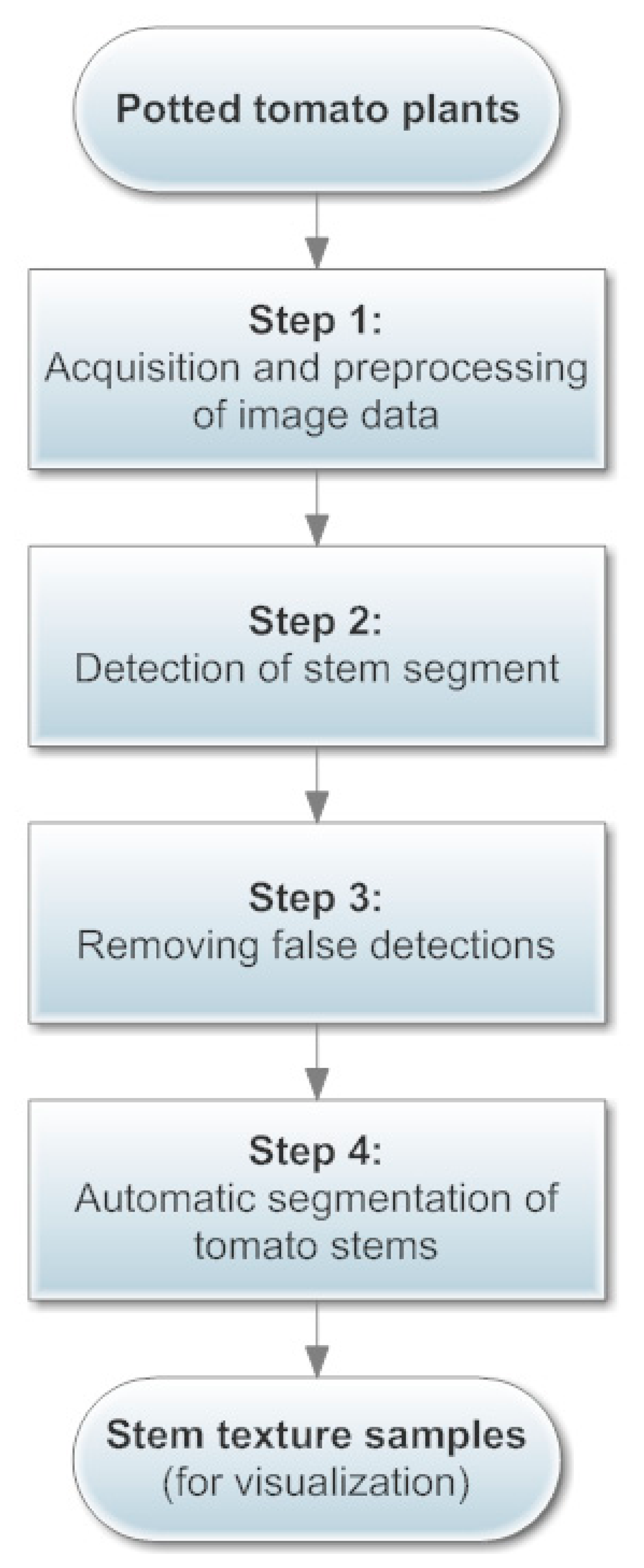
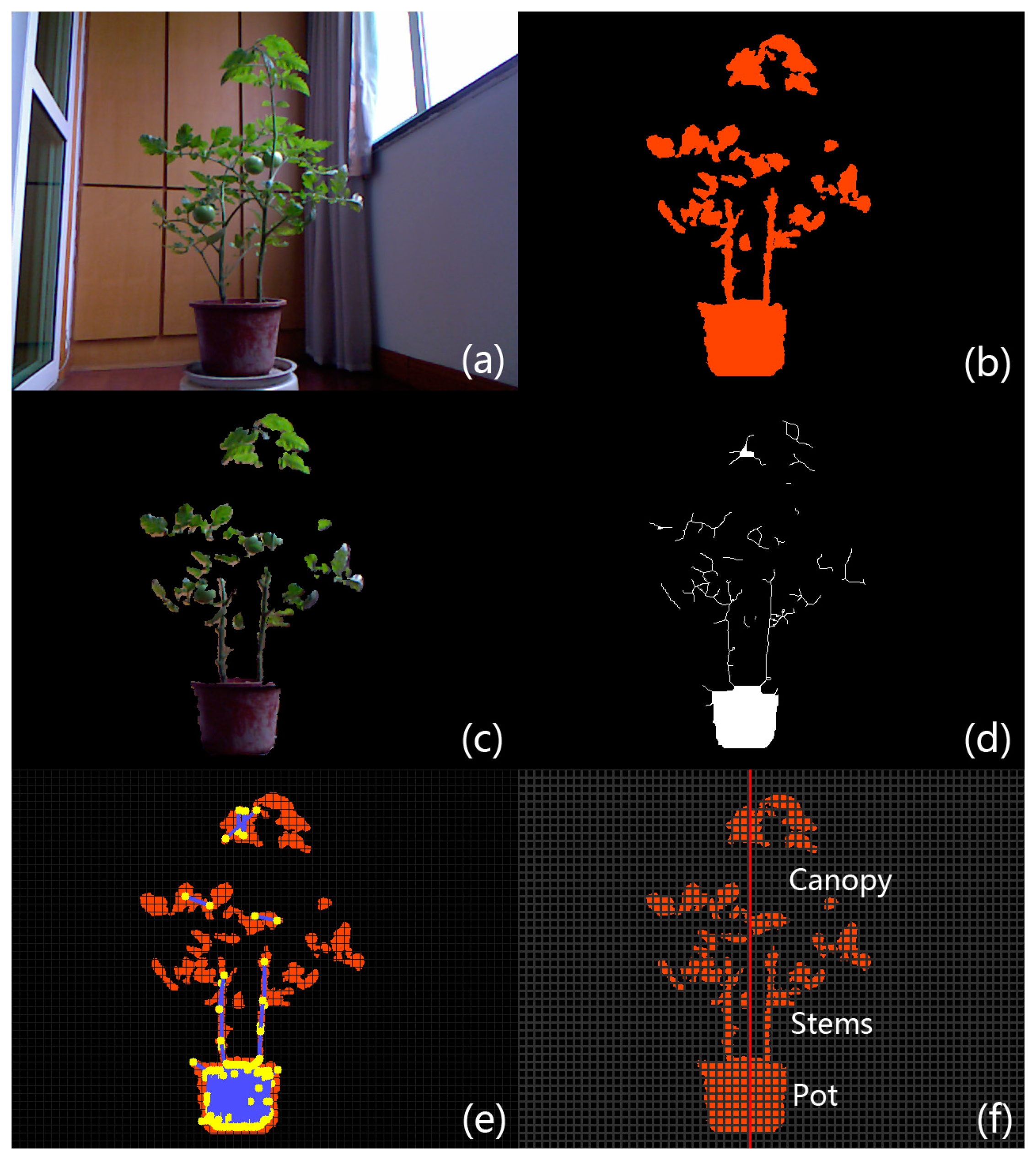
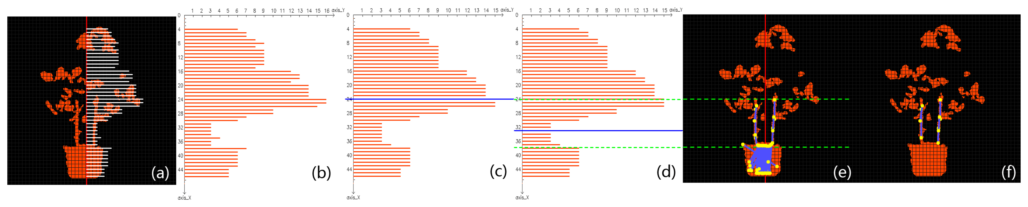
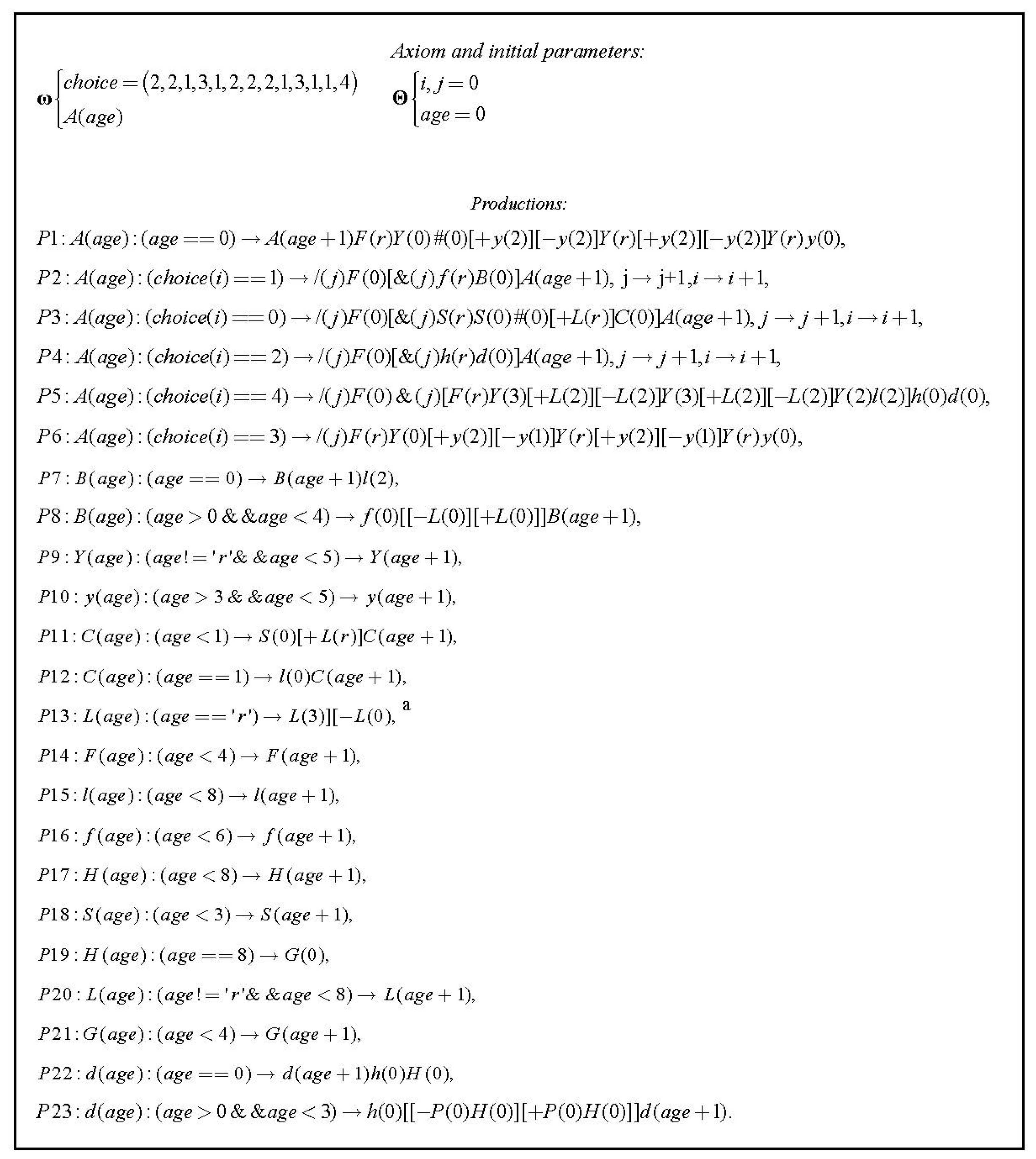
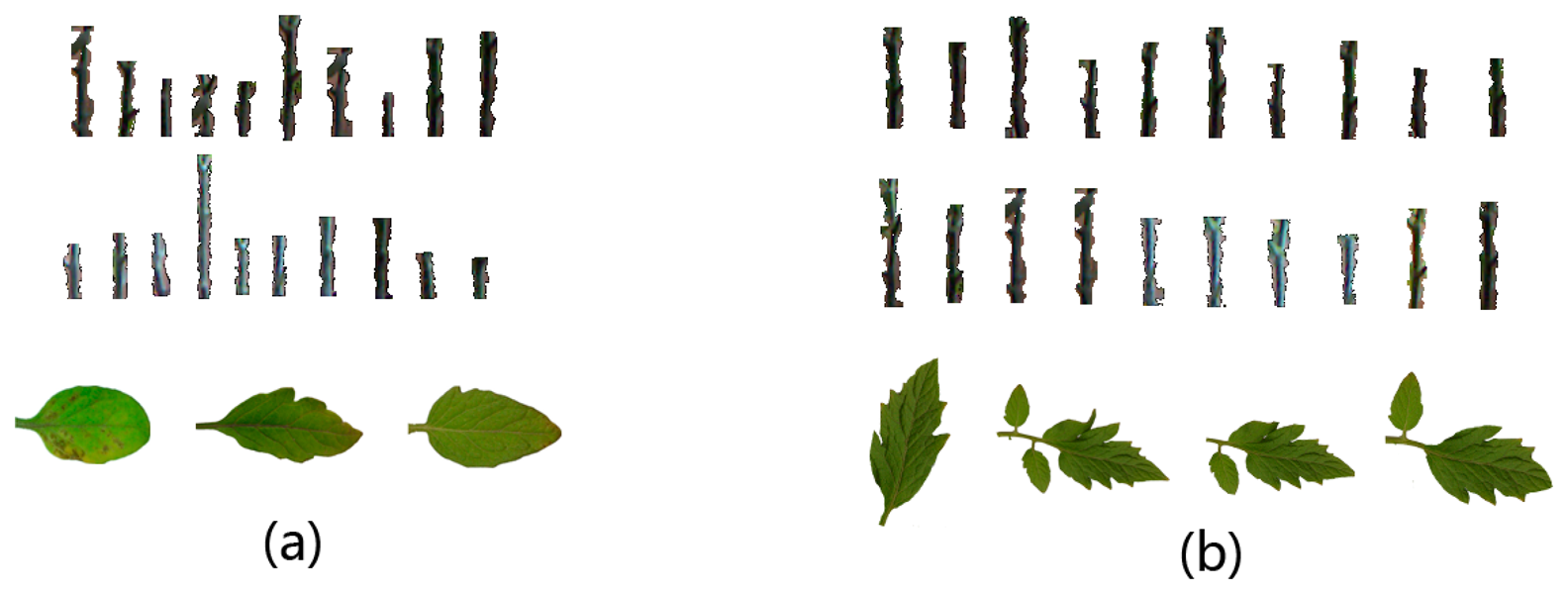
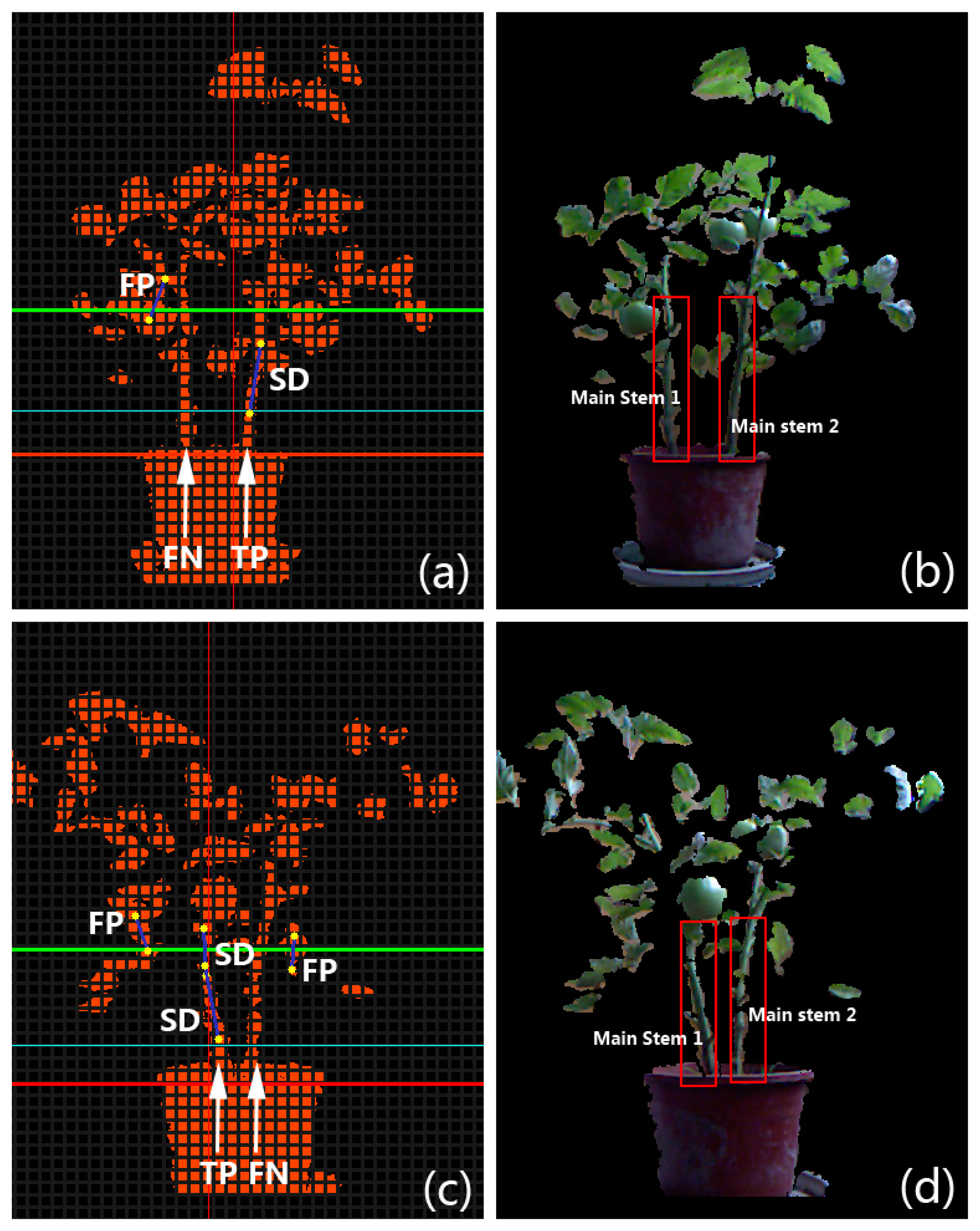
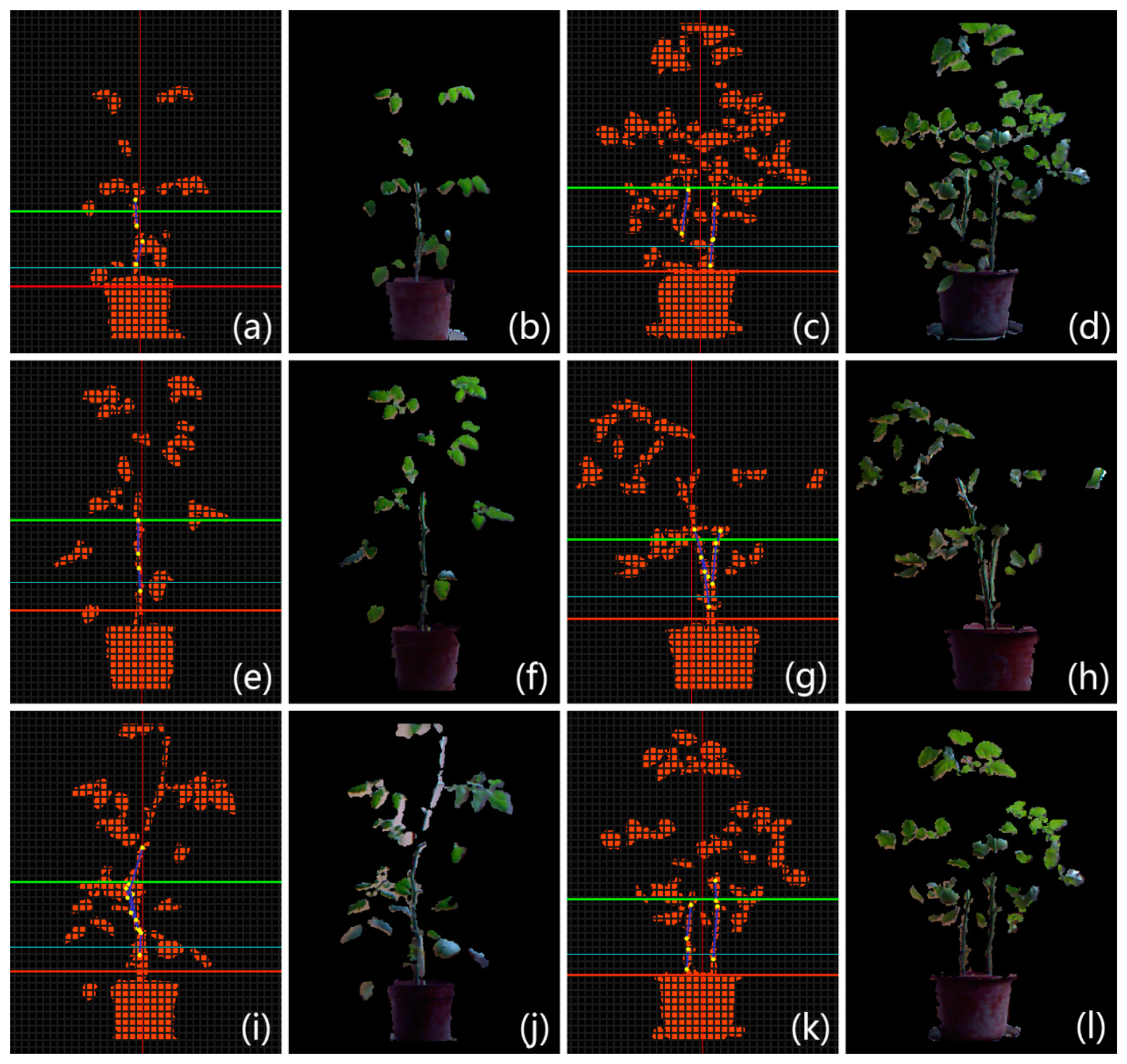
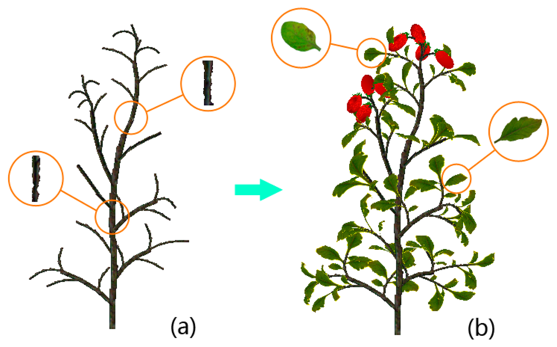
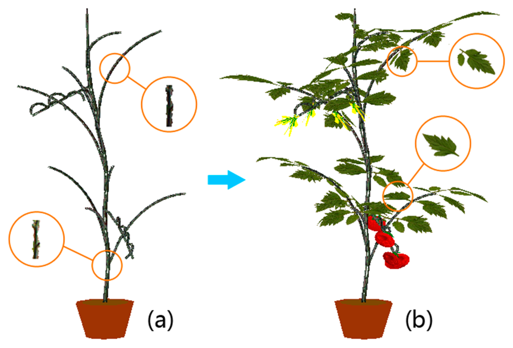
| Symbols | |
|---|---|
| L | Leaf that grows on the side of the branch |
| l | Leaf at the end of the lateral branch |
| F | Main stem |
| S | Short lateral branch (type 1) |
| G | Fruit |
| P | Flower stalk |
| H | Flower |
| Y | Bud stalk atop the main stem |
| y | Bud atop the main stem |
| h | Lateral branch with flower (type 3) |
| f | Lateral branch without flower (type 2) |
| Parameters | |
| age | Age of an organ or a component in the plant |
| r | A special state of the “age” parameter a |
| i | Index for traversing the “choice” string |
| j | Cumulative number for main stem growth |
| Operators: b | |
| / | An angle of curvature of the main stem |
| & | An spatial angle of lateral branch |
| # | An spatial angle of a leaf on the lateral branch |
| [ ] | A branching structure c |
| +,− | A rotation angle, positive for counterclockwise |
| &&,‖,==,!= | The same as defined in c++ language |
| Control character: d | |
| A | Main stem control character |
| B | Lateral branch control character |
| C | Control character of the shorter lateral branch |
| D | Control character of a full-fledged branch |
aFor all organs but leaves, age = r means they have reached a stable state and their morphological properties then remain unchanged; however, for a leaf, age = r means that at the next recursion, that leaf will be replaced by two leaves as a result of bifurcation (see production P13 in Figure 4);bWhen an operator is used for a change in spatial angle, we mean the subject of that operator is changed by that angular amount relative to the reference;cIn an L-system string, left and right brackets must appear in pairs, and a pair of “[ ]” stands for a branching structure which can be a lateral branch, a flower branch, or a leaf;dUnlike symbols, control characters do not have corresponding entities in visualization, but they can turn into different organ symbols in recursion. The main purpose of a control parameter is controlling a specific type of symbol.
| Cherry Tomato Plants | Ordinary Tomato Plants | ||||||
|---|---|---|---|---|---|---|---|
| Phase 1 | Phase 2 | Phase 3 | Phase 1 | Phase 2 | Phase 3 | Phase 4 | |
| Number of image pairs tested | 11 | 17 | 22 | 10 | 13 | 32 | 25 |
| Number of main stems | 11 | 17 | 22 | 19 | 24 | 63 | 47 |
| Number of detected stems | 14 | 16 | 33 | 18 | 21 | 78 | 48 |
| FN | 2 | 5 | 4 | 5 | 9 | 10 | 18 |
| TP | 9 | 12 | 18 | 14 | 15 | 53 | 29 |
| FP | 0 | 0 | 1 | 1 | 0 | 3 | 5 |
| SD | 14 | 16 | 32 | 17 | 21 | 75 | 43 |
| FNR | 18.2% | 29.4% | 18.2% | 26.3% | 37.5% | 15.9% | 38.3% |
| TPR | 81.8% | 70.6% | 81.8% | 73.7% | 62.5% | 84.1% | 61.7% |
| ER | 0.0% | 0.0% | 3.1% | 5.6% | 0% | 3.8% | 10.4% |
| Ac | 100.0% | 100.0% | 96.9% | 94.4% | 100.0% | 96.2% | 89.6% |
| Total FNR | 22.0% | 27.5% | |||||
| Total TPR | 78.0% | 72.5% | |||||
| Total ER | 1.6% | 5.5% | |||||
| Total Ac | 98.4% | 94.5% | |||||
© 2015 by the authors; licensee MDPI, Basel, Switzerland. This article is an open access article distributed under the terms and conditions of the Creative Commons Attribution license ( http://creativecommons.org/licenses/by/4.0/).
Share and Cite
Li, D.; Xu, L.; Tan, C.; Goodman, E.D.; Fu, D.; Xin, L. Digitization and Visualization of Greenhouse Tomato Plants in Indoor Environments. Sensors 2015, 15, 4019-4051. https://doi.org/10.3390/s150204019
Li D, Xu L, Tan C, Goodman ED, Fu D, Xin L. Digitization and Visualization of Greenhouse Tomato Plants in Indoor Environments. Sensors. 2015; 15(2):4019-4051. https://doi.org/10.3390/s150204019
Chicago/Turabian StyleLi, Dawei, Lihong Xu, Chengxiang Tan, Erik D. Goodman, Daichang Fu, and Longjiao Xin. 2015. "Digitization and Visualization of Greenhouse Tomato Plants in Indoor Environments" Sensors 15, no. 2: 4019-4051. https://doi.org/10.3390/s150204019