1. Introduction
Inline measurement of the component concentrations is an important approach to supervise industrial processes. Based on the concentration information, the process controls can be implemented and the stable product quality, the processing efficiency and the energy saving can be ensured [
1]. Nevertheless, the measurement of component concentrations in multicomponent mixtures cannot be easily achieved through a low-cost and inline technique. So far, several methods have been proposed to measure component concentrations. The sampling method [
2] is used to measure the local solid concentration based on separate solid and liquid phases, so it is not suitable for inline measurement. The multi-physics field combined methods [
3,
4] are accurate, but they confront one with the problems of high cost and complexity. It is still necessary to develop simple and low-cost methods. Ultrasonic sensor can satisfy the requirements of good robustness, high accuracy, inline measurement, safety and low maintenance in industrial processes [
5]. In recent years, the ultrasonic sensor has been successfully used to measure the concentration of mixtures. For binary mixtures, the ultrasonic features (e.g., ultrasonic attenuation and velocity) are directly correlated with concentrations [
6,
7]. However, it is very difficult or even impossible to derive a physical model to characterize the relationship between ultrasonic features and component concentrations in multicomponent mixtures [
8].
The variations of component concentrations have effects on the physical properties of multicomponent mixtures, including density, viscosity and bulk modulus [
9]. So the ultrasonic waves (amplitude and shape) transmitted through the multicomponent mixtures will also change along with the component concentrations, and, in turn, it is possible to measure the component concentrations through analyzing the ultrasonic signals. Some researchers have studied the possibility that the ultrasonic sensor is used to measure the component concentrations in multicomponent solutions. Resa
et al. [
10] have proposed the monitoring of alcoholic fermentation processes based on the combination of ultrasound velocity and semi-empirical models. Krause
et al. [
1,
11] have put forward a multivariate regression method for simultaneous detection of sugar and ethanol concentrations in aqueous solutions. Schafer
et al. [
8] reported that the partial least square (PLS) model could be used to estimate the concentration of sodium chloride in an aqueous solution by analyzing spectra of ultrasonic pulses. This research suggests that it is feasible to measure component concentrations in some solutions using ultrasonic sensors by means of multivariate analysis, but the ultrasonic measurement of component concentrations in multicomponent suspensions has been rarely reported.
The ultrasonic transmission mechanism of multicomponent suspensions is far more complex than that of multicomponent solutions [
12]. In multicomponent suspensions, the ultrasonic features and the component concentrations exhibit a nonlinear relationship because of the strong interactions among components. The statistical multivariate methods, such as the PLS model and the multiple linear regression (MLR) model, are not necessarily good options for modeling the nonlinear relationship between the features and target values [
13]. While the advanced models (such as the artificial neural network (ANN) approach and the LS-SVM model) are commonly applied to nonlinear systems as alternative solutions. Li
et al. [
14] presented an ultrasonic method to measure the liquid pressure and in that work, the ANN was employed to improve the measurement accuracy. The ANN has a disadvantage that the available sample set should be considerably large for the purpose of effective ANN training, while the LS-SVM model can build the model using a small sample set [
15]. In addition, with the help of kernels, the LS-SVM model is capable of modeling the nonlinear system in high-dimensional feature spaces with fewer training data [
16]. The LS-SVM has been effectively applied to inline estimate the biomass in fermentation process [
17], quantify the common adulterants in powdered milk [
18], and predict the milk-to-plasma drug concentration ratio [
19],
etc. Although the establishment of a LS-SVM model is time-consuming, once the model is established, the analysis can be completed within a short time [
20]. Therefore, the LS-SVM model is a promising technique for inline measurement of the particle concentrations in multicomponent suspensions.
Ultrasonic signals contain a wealth of information, but some information doesn’t contribute to the prediction of particle concentrations. Therefore, it is necessary to exclude non-informative and unimportant features that strongly affect the model stability [
11]. Then, the robustness and accuracy of model can be improved and while the complexity of model can be reduced [
21].
This paper is aimed to develop a new inline measurement system for simultaneous measurement of two particle concentrations in ternary suspensions based on ultrasonic sensor and the LS-SVM model. The features are collected from ultrasonic signals of time and frequency domains at first. Then the LS-SVM model is tuned, trained and tested to realize rapid inline prediction of the particle concentrations through some ultrasonic features. In addition, the comparative analysis between the PLS model and the LS-SVM model is conducted to give some insight into the two methods. Finally, the optimal LS-SVM model and the optimal feature subset are applied to inline measurement of particle concentrations in the mixing process. The proposed method is simple and easy to implement and can be extended to detecting the mixtures of more components. As far as the authors are concerned, this is a pioneering project in the field of concentration measurements of multicomponent suspensions, which makes it possible to carry out inline monitoring for production processes and product quality in multicomponent suspensions with only one ultrasonic sensor.
3. Results and Discussion
3.1. Data Pre-Processing
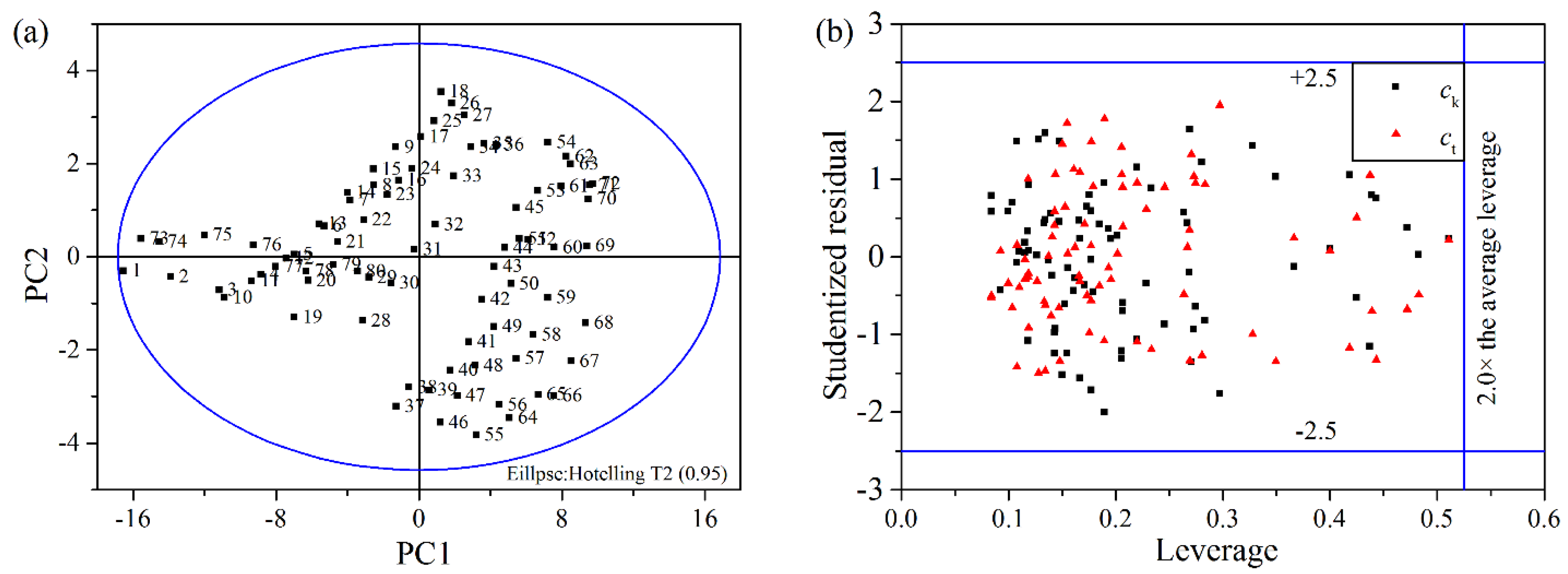
Because of the potential influences of bubbles and impurities as well as the complex characteristics of suspensions in industrial process, the detection of outliers is very critical in data pre-processing [
28]. In this paper, the scatter plot of the first two principal components (PC1 and PC2) is used to detect the potential outlier(s). The scatter plot is a map of the target values, displaying how the features are situated with respect to each other. The samples situated outside the tolerance ellipse based on Hotelling’s T2 are considered as outliers [
29]. As shown in
Figure 4a, no samples are flagged and demonstrated to be outliers and the samples are not overlapped and can be clearly separated in scatter plots.
Leverage analysis is also used as an additional diagnostic tool for outliers, which reflects differences between a sample spectrum and the average spectrum of the sample set [
30]. The concentration residuals are scaled by the standard deviation of the residuals to generate the studentized residuals. The relationship between the leverage and the studentized residual is shown in
Figure 4b. The outliers are flagged at ±2.5 studentized residuals and the double of the average leverage [
31]. As shown in
Figure 4b, no samples are flagged and demonstrated to be outliers in accordance with the analysis above.
Figure 4.
(a) The scatter plot of principal components (PC1/PC2); (b) The scatter plot of the leverage and the studentized residual.
Figure 4.
(a) The scatter plot of principal components (PC1/PC2); (b) The scatter plot of the leverage and the studentized residual.
There are 54 ultrasonic features for each sample. All features can be used to establish the LS-SVM model or the PLS model, but irrelevant or incorrect features may have adverse impacts on the generalization performance. The feature selection based on the importance of features in the model can not only reduce the dimensionality of data but also improve the prediction performance.
The importance of features, which is calculated with a combination of VIP and SRC, serves as the basis of feature selection. The absolute values of VIP and SRC of each feature are normalized into the region [0, 1] and denoted as VIP’ and SRC’, respectively. The sum of VIP’ and SRC’ gives an indication of how important the features are to the target values. All features are arranged in the decreasing order of importance (
Figure 5). It shows that time distribution features (
T8–
T12) and frequency distribution features (
F9–
F12) are insensitive or irregular in correlation to the particle concentrations.
Figure 5.
The importance of each feature.
Figure 5.
The importance of each feature.
According to the importance of the features, the unimportant features are excluded sequentially and new feature subsets (
Table 2) are re-grouped. M1 subset contains all features (see
Table 1). M2 and M3 subsets include all time domain and frequency domain features, respectively. M4 subset contains all time domain features excluding
T8–
T12, and M5 contains all frequency domain features excluding
F9–
F12. M6 subset is the combination of M4 and M5 subsets. All subsets are used to build the model and find out the optimal feature subset that shows the best performance.
Table 2.
The feature subset summaries.
Table 2.
The feature subset summaries.
| Subset | Time Features | Frequency Features | Count |
|---|
| M1 | | | 54 |
| M2 | | / | 20 |
| M3 | / | | 34 |
| M4 | | / | 15 |
| M5 | / | | 30 |
| M6 | | | 45 |
3.2. Optimization of Model Parameters
According to the analysis above, the optimization of parameters γ and σ2 is the critical step to obtain the optimal LS-SVM model. In this study, the iterative grid search is performed to find the parameter range. For each combination of (λ, σ2) (grid point), the 10-fold cross-validation is used to calculate the prediction errors using the training set. The optimum parameters are selected which produce smallest prediction errors.
The grid search is a gradual search process. The first step is a crude search with a large size, while the next step is conducted with a smaller size than the previous step until it meets the search conditions. The result of the grid search is an error surface spanned by the model parameters, and the color stand for RMSEV values. With the parameters in a smooth area, a robust model can be built. Hence, the optimal parameters are selected from a smooth subarea with the lowest RMSEV. After the grid search, the optimal combination of (λ, σ
2) is achieved for the LS-SVM models. The contour plot for the optimization process of parameters γ and σ
2 for M5 feature subset is shown in
Figure 6. The search process has been completed through only two steps (two iterations). For the M5 feature subset, the optimal combinations of (λ, σ
2) are found to be (1.1545 × 10
5, 114.9) and (1.4978 × 10
5, 125.5587) for
ck and
ct, respectively. In the same way, the optimal combinations of (λ, σ
2) for other feature subsets can be found.
Figure 6.
The contour plot of RMSEV versus γ and σ2 in the grid search for (a) ck and (b) ct. The grids “·” and “+” are 10 × 10 in the first step and the second step, respectively. The color stand for the value of RMSEV.
Figure 6.
The contour plot of RMSEV versus γ and σ2 in the grid search for (a) ck and (b) ct. The grids “·” and “+” are 10 × 10 in the first step and the second step, respectively. The color stand for the value of RMSEV.
The PLS model is used as the reference method in this study. The PLS model is a common and useful tool for modeling the relationship between the features and the target values. The model order (the number of PCs) of the PLS model is important to achieve good performance.
, which is the average RMSEP of
ck and
ct, is used to determine the optimal number of PCs. For each feature subset, the PLS model is built and
is calculated (
Figure 7). It can be seen that all models start with high
values but decrease rapidly at first and then decrease smoothly. The
values become asymptotic around 10–15 factors, but the minimums are different. The optimum number of PCs which produces the smallest
can be easily found in
Figure 7 and then used to construct the PLS model.
Figure 7.
of each feature subset against the number of PCs
Figure 7.
of each feature subset against the number of PCs
3.3. Model Training and Testing
Using the optimum parameters γ and σ
2, the LS-SVM models for
ck and
ct are trained for each feature subset using the training subset, respectively. To investigate the prediction ability of the model, the model is used to measure the particle concentrations in prediction subset, which doesn’t contribute to the model building. The performance of the LS-SVM model (
and RMSEP) is calculated and showed in
Table 3. For the comparison among six feature subsets, the best performance is achieved with M5 subset. In the optimal model and selection of features, RMSEP of the LS-SVM model is 0.31 wt% for Kaolin and 0.34 wt% for TiO
2. The maximum absolute residual errors
) in prediction subset of Kaolin and TiO
2 are less than 0.45 wt% and 0.56 wt%, respectively. Based on the results above, it can be concluded that the combination of ultrasonic sensor and the LS-SVM model is a reliable and accurate method for the prediction of particle concentrations in multicomponent suspensions.
The PLS models are built using the same sample subsets as the LS-SVM models and the optimal parameters which have the smallest
shown in
Figure 7. The performance comparison between the PLS model and the LSV-SVM model is shown in
Table 3. RMSEP and R
2 of the optimal PLS model, namely 0.52 wt% and 0.995 for
ck, 0.67 wt% and 0.989 for
ct, are larger and less than those of the LS-SVM model, respectively, which indicates that the prediction performance of the LS-SVM model is better than that of the PLS model. The PLS model is suited to the linear system, while the LS-SVM model is commonly used in the nonlinear system. Hence, the reason why the LS-SVM model produces higher prediction accuracy than the PLS model may be the presence of nonlinear relationship between ultrasonic features and component concentrations.
Table 3.
The performance of the partial least square (PLS) model and the least squares support vector machines (LS-SVM) model.
Table 3.
The performance of the partial least square (PLS) model and the least squares support vector machines (LS-SVM) model.
| Feature Subset | PLS | LS-SVM |
|---|
| RMSEP_ck | _ck | RMSEP_ct | _ct | RMSEP_ck | _ck | RMSEP_ct | _ct |
|---|
| M1 | 0.0068 | 0.993 | 0.0075 | 0.988 | 0.0057 | 0.994 | 0.0081 | 0.984 |
| M2 | 0.0060 | 0.994 | 0.0098 | 0.977 | 0.0065 | 0.993 | 0.0091 | 0.980 |
| M3 | 0.0058 | 0.996 | 0.0092 | 0.980 | 0.0056 | 0.994 | 0.0156 | 0.943 |
| M4 | 0.0055 | 0.996 | 0.0089 | 0.982 | 0.0048 | 0.996 | 0.0088 | 0.982 |
| M5 | 0.0069 | 0.993 | 0.0124 | 0.964 | 0.0031 | 0.999 | 0.0034 | 0.998 |
| M6 | 0.0052 | 0.995 | 0.0067 | 0.989 | 0.0030 | 0.999 | 0.0041 | 0.996 |
In addition, through the selection of suitable model parameters, the LS-SVM model and the PLS model have good prediction capabilities. After excluding the non-informative and unimportant features, the prediction accuracies of both models are further improved. With all features (M1), the LS-SVM model performs slightly better than the PLS model. However, after feature selection (M4, M5 and M6 subsets), the LS-SVM model generates a better prediction performance than the PLS model. The PLS model and the LS-SVM model have the best prediction performances for M6 subset (44 features) and M5 subset (30 features), respectively. The further removal of features causes a reduction of the accuracy due to the lack of sufficient information for the model, and the further addition of features also degrades the performance because of the addition of redundant “noise” to the model. Hence, it can be concluded that the selection of appropriate features is crucial to the model performance, which can reduce the system dimension and improve the model accuracy.
With the optimal model parameters and optimal feature subset, the plots of actual concentrations against prediction concentrations for the training and prediction subsets using the PLS model and the LS-SVM model are shown in
Figure 8. The results show the points tend to cluster along the lines close to the 45° tangent line, which reflects an acceptable model adequacy. It can be easily seen that the LS-SVM model gives both better fitting and prediction results. In the LS-SVM model, all points of the plots fall on or close to the unity line, which suggests that the prediction capability of the model is good and the over-fitting problem is not obvious. It can also be found that the prediction values of the PLS model have significant errors for the samples, which only contain one component in the suspensions. However, the LS-SVM model presents an excellent prediction capability in the full concentration range. The sudden changes of features occur when the components of suspensions change from two to three. The LS-SVM model is not only capable of modeling the main linear relationship but also can grasp the nonlinear relationship existing in real data, thus leading to more accurate predictions. The PLS model is inherently a linear modeling method, which makes it impossible to well account for the nonlinear relationship of the data.
Figure 8.
The predicted values vs. the actual values using (a) the optimal PLS model and (b) the optimal LS-SVM model.
Figure 8.
The predicted values vs. the actual values using (a) the optimal PLS model and (b) the optimal LS-SVM model.
3.4. Inline Measurement
The inline measurement of particle concentrations in multicomponent suspensions is of great importance. The combination of ultrasonic sensor and the LS-SVM model provides an alternative method to inline measure the particles concentration.
In order to evaluate the inline measurement ability of the model, an independent inline measurement is implemented. In this process, the real-time ultrasonic signals are acquired with an interval of 1 s after the suspensions become homogeneous. A time-moving window with a length of 10 s is used to average the signals. In the process, as the new data are added into the window, the oldest data are disposed. Then, the resulting signals are processed by the transformations mentioned above (average, window, zero-pad and FFT). The ultrasonic features are selected in accordance with the M5 subset. After auto scaling, the data set is statistically analyzed to determine outliers, which aim to decide whether the sample is within the scope of the model or not. With the optimal model parameters, the LS-SVM model is used to inline measure the intently-designed samples (the data are not used in model development, see
Figure 3).
The results of inline measurement are shown in
Figure 9. As shown in
Figure 9a, the concentrations of two real-time measurements are obviously fluctuant, and specifically,
ct shows more fluctuant changes than
ck. Compared with the offline predicted results in
Figure 8, the error of inline concentration measurement is larger, which is mainly caused by the dynamic measurement along with the fluctuation of signals. The noise disturbance cannot be eliminated through the mean method in consideration of real-time measurement, and accordingly the accuracy of concentration measurement is reduced. Nevertheless, the errors of concentration measurements of Kaolin and TiO
2 in inline test subset are less than ±0.65 wt% and ±0.80 wt% respectively, which meet the industrial requirements.
In
Figure 9b, the black points and the red points represent the actual concentrations and the averaged concentrations for 5 min, respectively. The error bars denote the concentration fluctuation in 5 min. The distance of two points in the same sample indicates the difference of two concentrations. As shown in
Figure 9b, the small distance between two points in the same sample demonstrates that the measurement has high accuracy when the mean method is used. In the event that the low real-time requirements are put forward, the measurement accuracy can be further improved through increasing the collection points or slip averaging the measurement results. The inline measurement performance shows that the LS-SVM model is capable of modeling nonlinear system dynamically.
Figure 9.
The result of inline measurement: (a) The real-time measurement concentration; (b) The XY error bar graph of the averaged ck and ct in 5 min.
Figure 9.
The result of inline measurement: (a) The real-time measurement concentration; (b) The XY error bar graph of the averaged ck and ct in 5 min.
4. Conclusions
This paper proposes an alternative methodology for inline measurement of particle concentrations in multicomponent suspensions based on a combination of ultrasonic sensor and LS-SVM model. The optimum feature subset that results in the best performance is found based on SRC and VIP values. According to the result of model evaluation, the measurement system has an acceptable accuracy. In comparison with the PLS model, the LS-SVM model with fewer features has a better prediction ability of particle concentrations in multicomponent suspensions. Furthermore, inline measurement is performed and the results reveal that the measurement accuracy is sufficiently high in the application of monitoring industrial processes. The proposed technique can easily be extended to detecting the mixtures of more components and provides a tool for process control where the complex system makes it difficult to build a reliable physical model.
In the future, related research will be carried out to take the superposition phenomena caused by temperature into consideration, further improve the measurement accuracy by increasing samples, and develop the inline monitoring technology for production process and product quality based on the inline concentration measurement.


