
Calorimetry Minisensor for the Localised Measurement of Surface Heat Dissipated from the Human Body


Abstract
:1. Introduction
2. Experimental Section
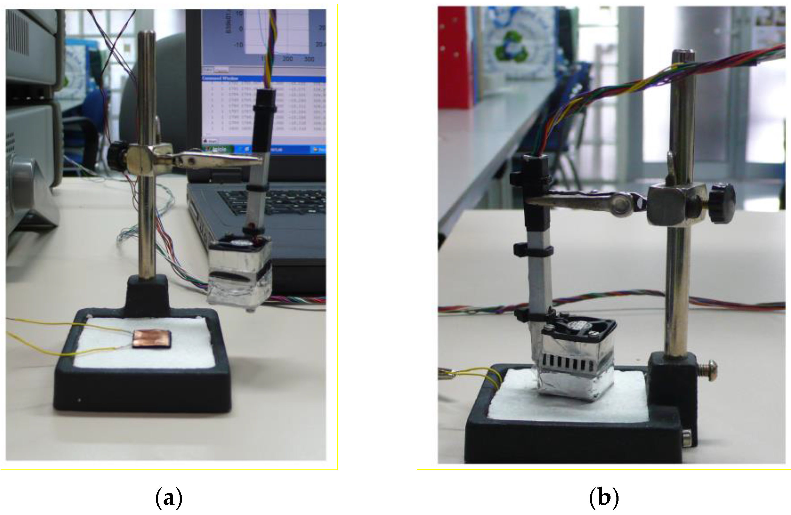
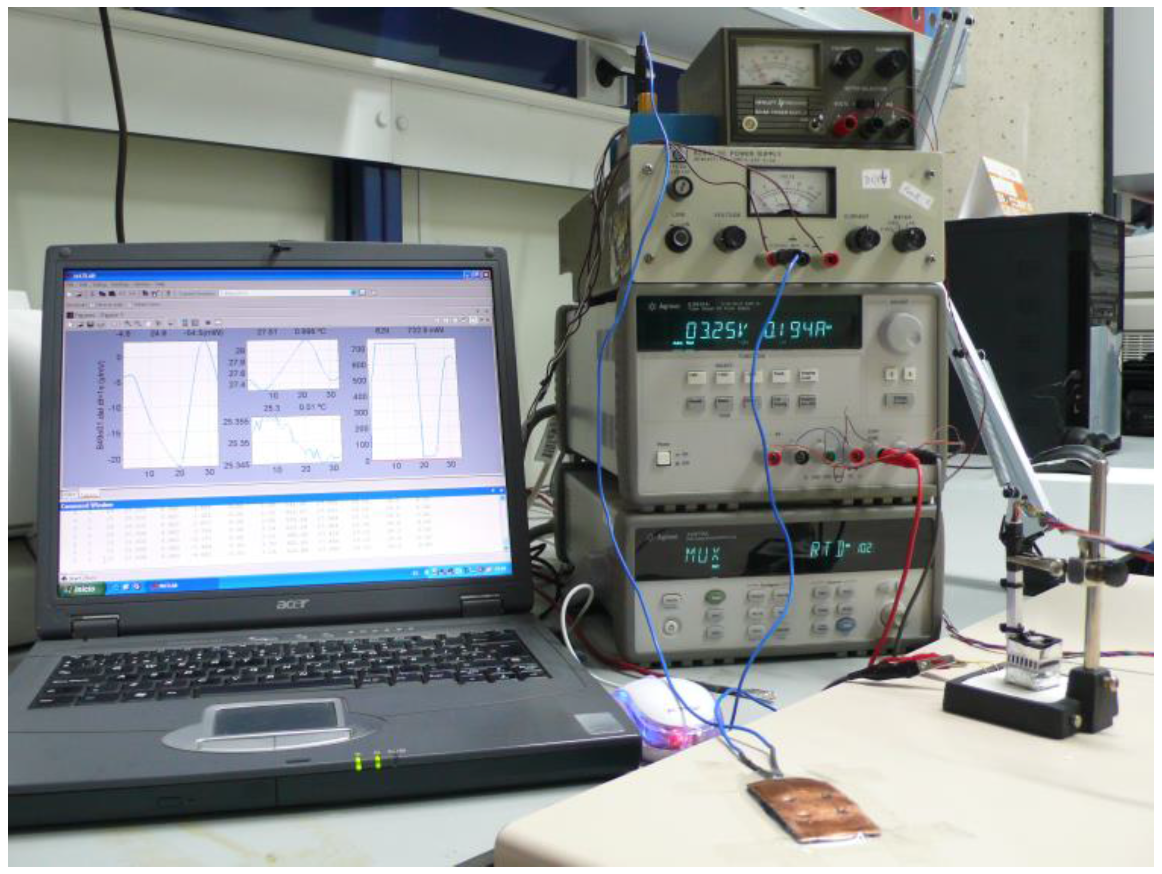
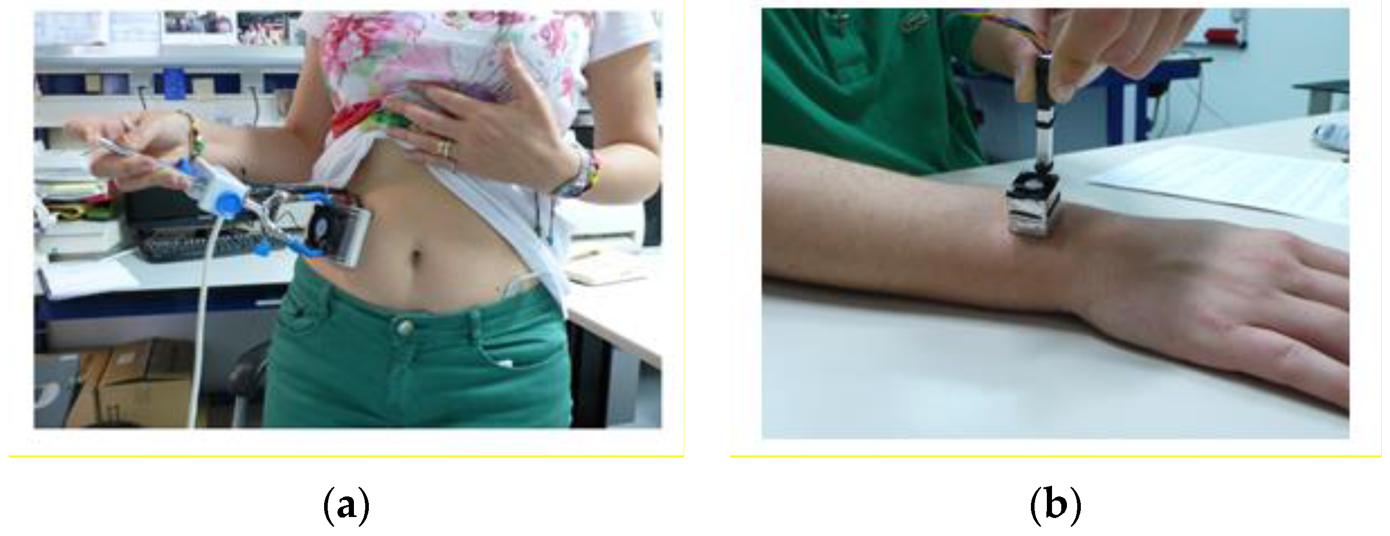
2.1. Sensor and Measurement and Control Instrumentation
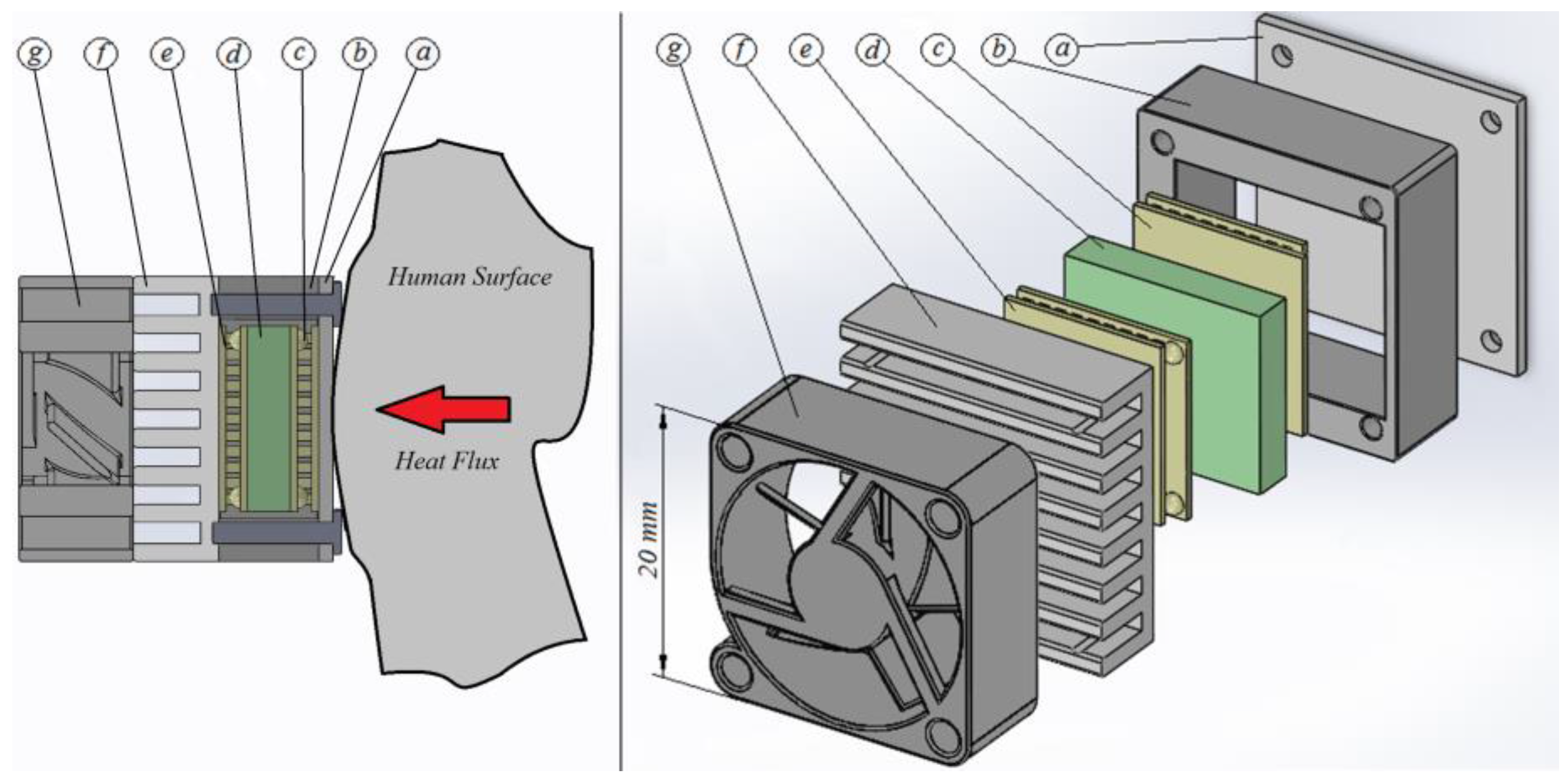
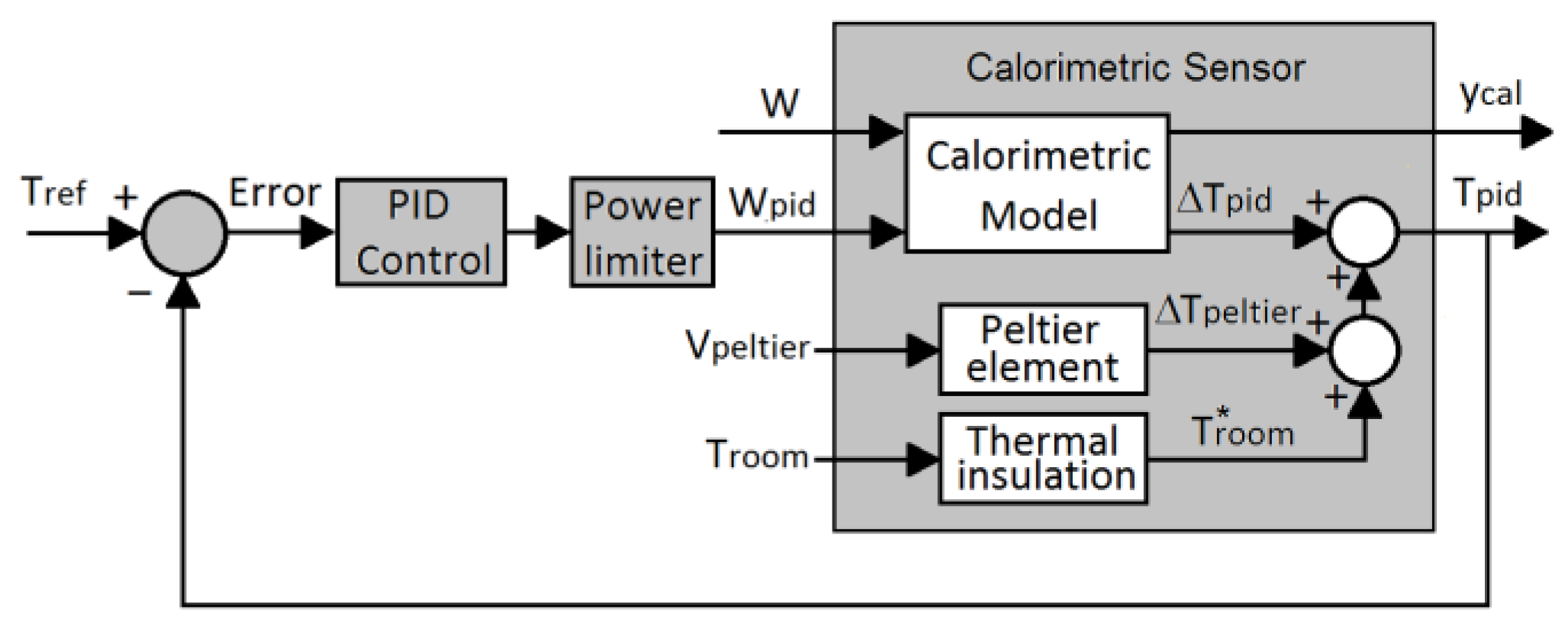
2.2. Sensor Operating Diagram
3. Sensor Modelling and Calibration
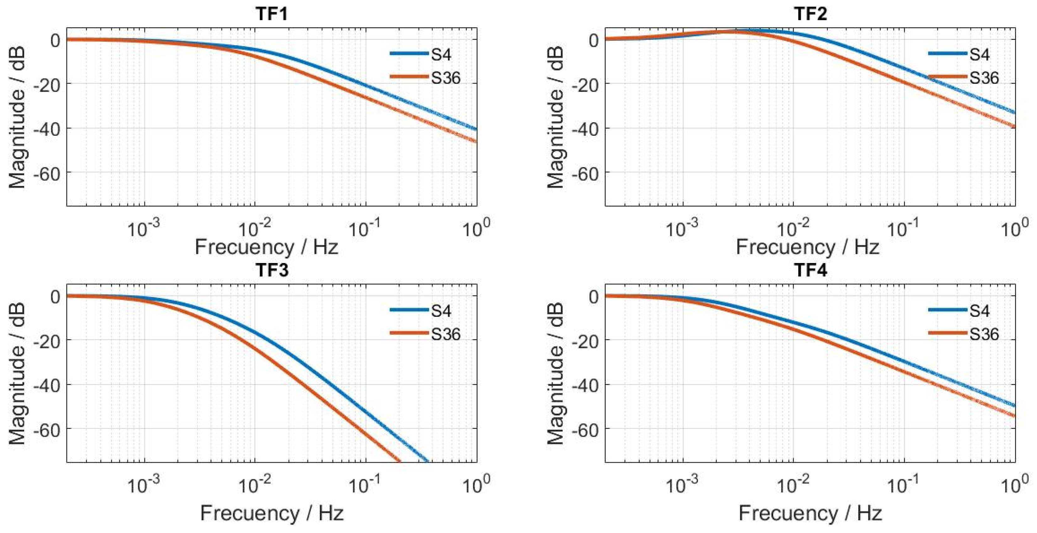
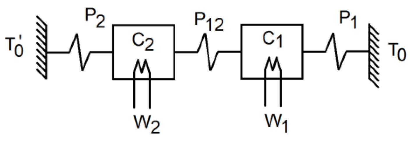
3.1. Modelling
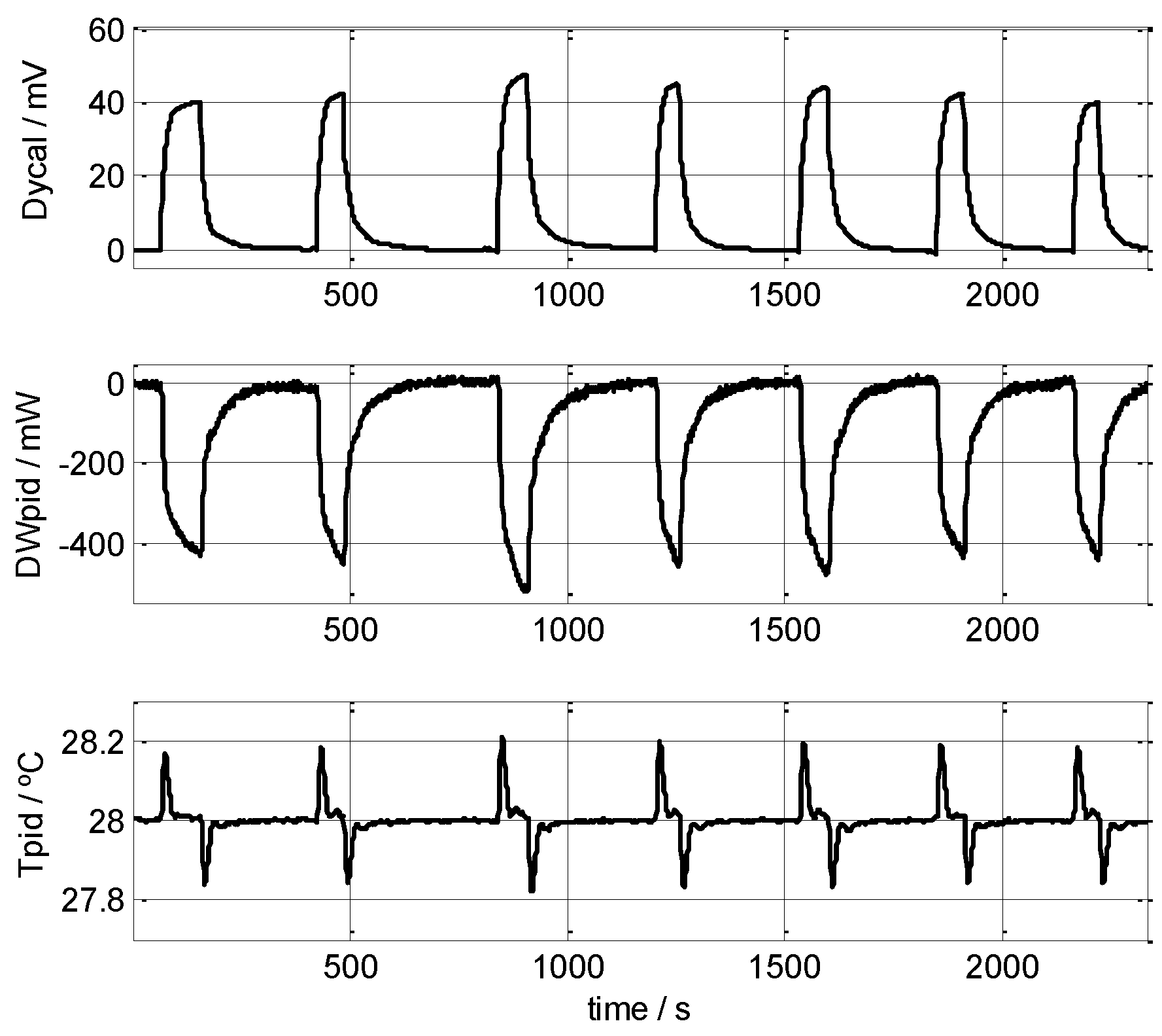
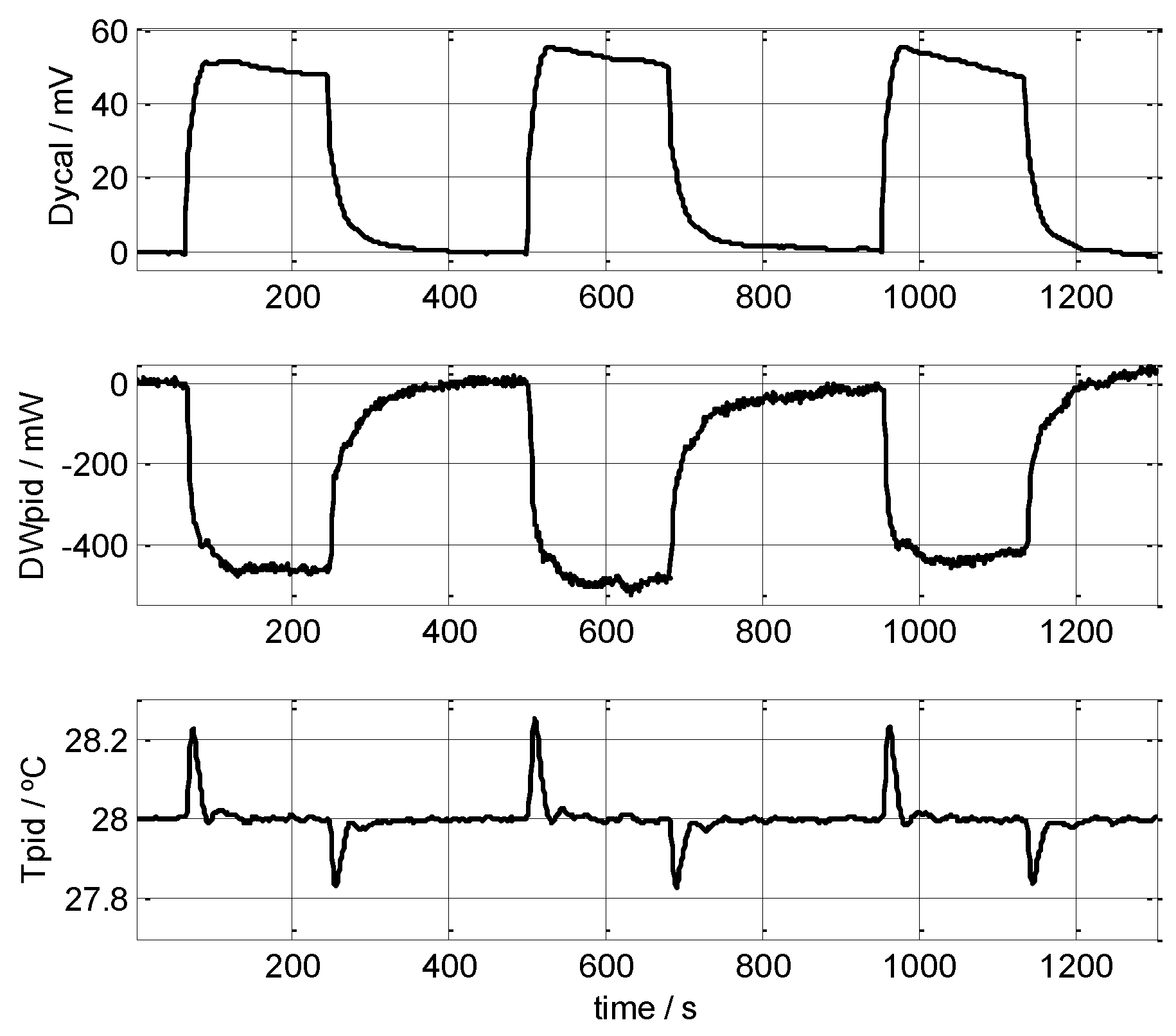
3.2. Calibration
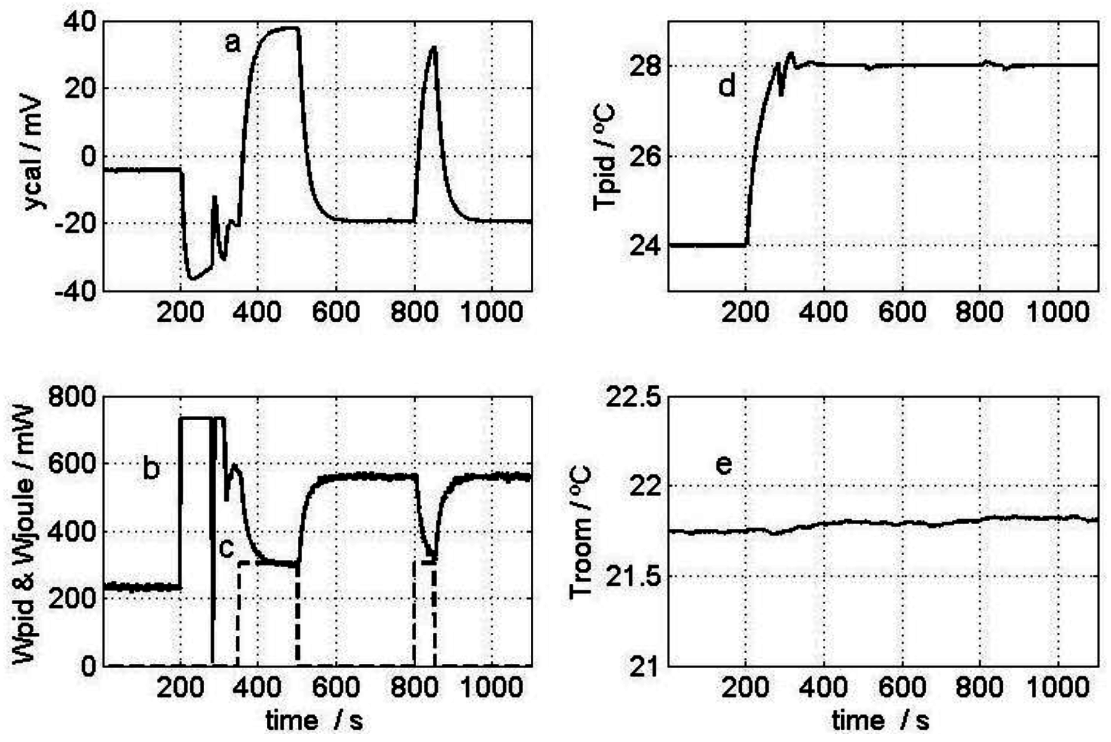
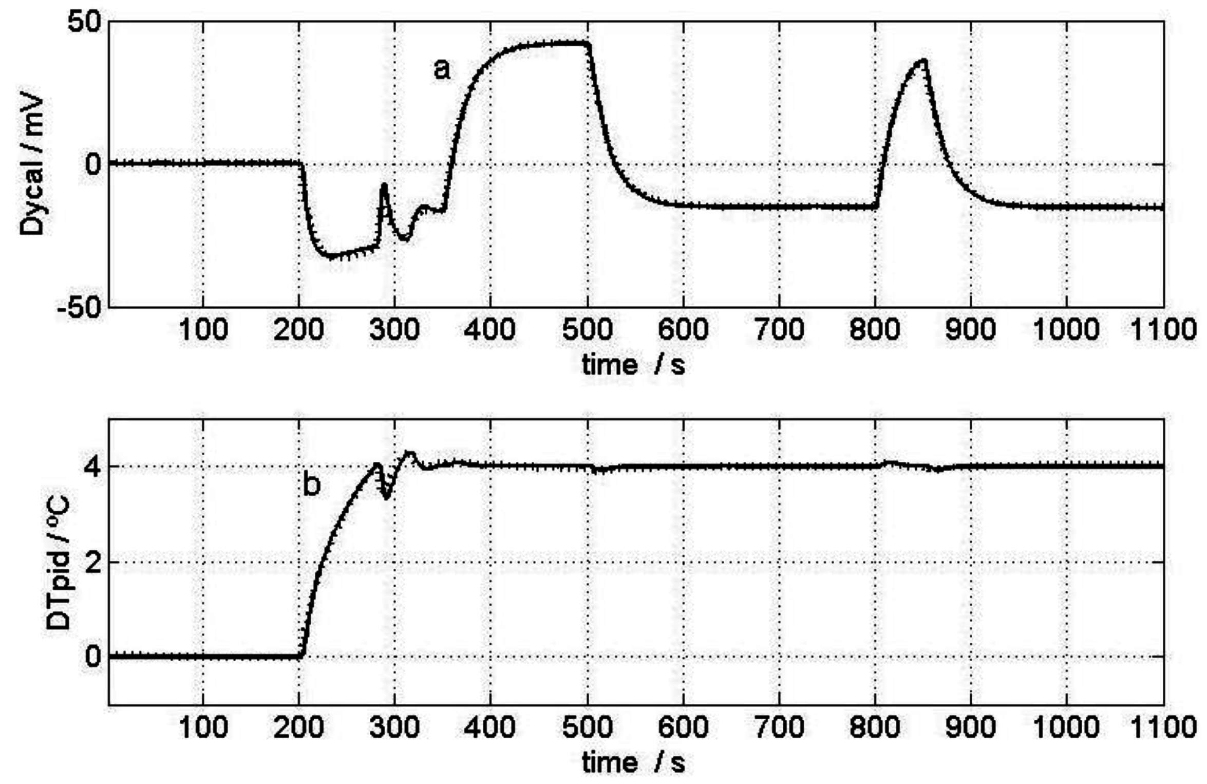
4. Results
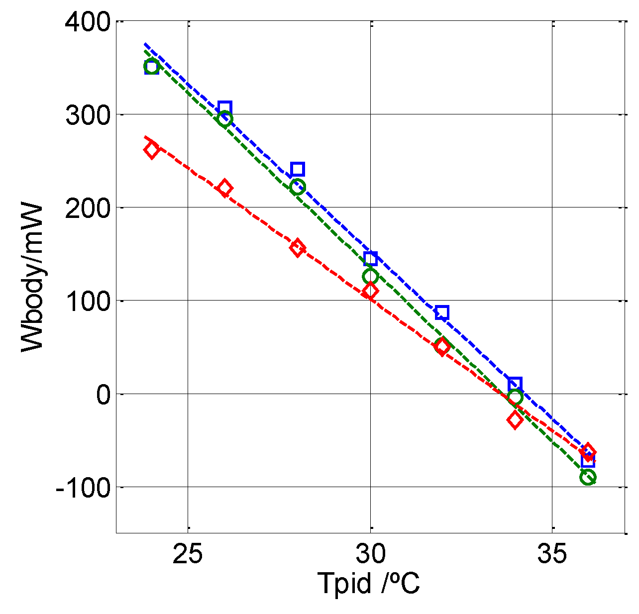
4.1. Method for Measuring and Calculating the Mean Power Dissipated from the Surface of the Human Body
4.2. Sensor Resolution and Operating Domain
5. Conclusions
Author Contributions
Conflicts of Interest
References
- Wendlandt, W.W. Thermal Methods of Analysis; John Wiley and Sons: New York, NY, USA, 1974. [Google Scholar]
- Brown, M.E. (Ed.) Handbook of Thermal Analysis and Calorimetry: Principles and Practice; Elsevier Science: Amsterdam, The Netherlands, 1998; Volume 1.
- Hansen, L.D. Toward a standard nomenclature for calorimetry. Thermochim. Acta 2001, 371, 19–22. [Google Scholar] [CrossRef]
- Socorro, F.; de Rivera, M.R. Development of a calorimetric sensor for medical application. Part I. Operating model. J. Therm. Anal. Calorim. 2010, 99, 799–802. [Google Scholar] [CrossRef]
- Jesús, C.; Socorro, F.; de Rivera, M.R. Development of a calorimetric sensor for medical application. Part II. Identification and Simulation. J. Therm. Anal. Calorim. 2013, 113, 1003–1007. [Google Scholar] [CrossRef]
- Jesús, C.; Socorro, F.; de Rivera, M.R. Development of a calorimetric sensor for medical application. Part III. Operating methods and applications. J. Therm. Anal. Calorim. 2013, 113, 1009–1013. [Google Scholar] [CrossRef]
- Jesús, C.; Socorro, F.; de Rivera, H.J.R.; de Rivera, M.R. Development of a calorimetric sensor for medical application. Part IV. Deconvolution of the calorimetric signal. J. Therm. Anal. Calorim. 2014, 116, 151–155. [Google Scholar] [CrossRef]
- Brooks, A.G.; Withers, R.T.; Gore, C.J.; Vogler, A.J.; Plummer, J.; Cormack, J. Measurement and prediction of METs during household activities in 35- to 45-year-old females. Eur. J. Appl. Physiol. 2004, 91, 638–648. [Google Scholar] [CrossRef]
- Kozey, S.; Lyden, K.; Staudenmayer, J.; Freedson, P. Errors in MET estimates of physical activities using 3.5 mL × kg(−1) × min(−1) as the baseline oxygen consumption. J. Phys. Act. Health 2010, 7, 508–516. [Google Scholar] [CrossRef]
- McLean, J.L.; Tobin, G. Animal and Human Calorimetry; Cambridge University Press: Cambridge, UK, 1987. [Google Scholar]
- Lamprecht, I. Calorimetry and thermodynamics of living systems. Thermochim. Acta 2003, 405, 1–13. [Google Scholar] [CrossRef]
- Hukseflux. Thermal Sensors. Available online: http://www.hukseflux.com/ (accessed on 4 November 2016).
- Leonov, V. Thermoelectric energy harvester on heated human machine. J. Micromech. Microeng. 2011, 21, 125013. [Google Scholar] [CrossRef]
- Carmo, J.P.; Antunes, J.; Silva, M.F.; Ribeiro, J.F.; Goncalves, L.M.; Correia, J.H. Characterization of thermoelectric generators by measuring the load-dependence behavior. Measurement 2011, 44, 2194–2199. [Google Scholar] [CrossRef]
- Ogata, K. Modern Control Engineering; Prentice Hall: Upper Saddle River, NJ, USA, 2010. [Google Scholar]
- Goodwin, G.C.; Graebe, S.F.; Salgado, M.E. Control System Design; Prentice Hall: Upper Saddle River, NJ, USA, 2001. [Google Scholar]
- Martin, J. Protocols for the high temperature measurement of the Seebeck coefficient in thermoelectric materials. Meas. Sci. Technol. 2013, 34, 085601. [Google Scholar] [CrossRef]
- Isalgue, A.; Ortin, J.; Torra, V.; Viñals, J. Heat flux calorimeters: Dynamical model localized time constants. An. Fis. 1980, 76, 192–196. [Google Scholar]
- Socorro, F.; de Rivera, M.R.; Jesús, C. A thermal model of a flow calorimeter. J. Therm. Anal. Calorim. 2001, 64, 357–366. [Google Scholar] [CrossRef]
- Kirchner, R.; de Rivera, M.R.; Seidel, J.M.; Torra, V. Identification of micro-scale calorimetric devices. Part VI. An approach by RC-representative model to improvements in TAM microcalorimeters. J. Therm. Anal. Calorim. 2005, 82, 179–184. [Google Scholar] [CrossRef]
- Nelder, J.A.; Mead, C. A simplex method for function minimization. Comput. J. 1965, 7, 308–313. [Google Scholar] [CrossRef]
- The MathWorks, Inc. Optimization ToolboxTM User’s Guide; 5th printing; Revised for Version 3.0 (Release 14); The MathWorks, Inc.: Natick, MA, USA, 2004. [Google Scholar]


| RC Model | TF Model | |||
|---|---|---|---|---|
| S4 Sensor | S4 Sensor | S36 Sensor | ||
| C1 | 2.9146 J·K−1 | K1 | 148.7 mV·W−1 | 46.0 mV·W−1 |
| C2 | 3.9735 J·K−1 | K2 | −45.4 mV·W−1 | −9.3 mV·W−1 |
| P1 | 0.0203 W·K−1 | K3 | 10.1 K·W−1 | 1.76 K·W−1 |
| P2 | 0.0663 W·K−1 | K4 | 12.0 K·W−1 | 1.70 K·W−1 |
| P12 | 0.1116 W·K−1 | τ1 | 82 s | 147 s |
| K | 24.6678 mV·K−1 | τ2 | 13 s | 27 s |
| Errors (Equation (11)) | τ1* | 60 s | 91 s | |
| σy | 29.5 µV | τ2* | 144 s | 243 s |
| σT | 1.5 mK | τ3* | 0 s | 0 s |
| N | 1100 points | τ4* | 22 s | 49 s |
| Tpid | Troom | VPeltier (V) | ΔTPeltier (°C) | Wmax (mW) |
|---|---|---|---|---|
| 26 °C | 20 °C | 0.51 | −2.64 | 855 |
| 25 °C | 1.26 | −7.64 | 855 | |
| 30 °C | 2.88 | −12.64 | 855 | |
| 28 °C | 20 °C | 0.26 | −0.64 | 855 |
| 25 °C | 0.93 | −5.64 | 855 | |
| 30 °C | 1.92 | −10.64 | 855 | |
| 30 °C | 20 °C | 0.04 | +1.36 | 855 |
| 25 °C | 0.64 | −3.64 | 855 | |
| 30 °C | 1.45 | −8.64 | 855 |
© 2016 by the authors; licensee MDPI, Basel, Switzerland. This article is an open access article distributed under the terms and conditions of the Creative Commons Attribution (CC-BY) license (http://creativecommons.org/licenses/by/4.0/).
Share and Cite
Socorro, F.; Rodríguez de Rivera, P.J.; Rodríguez de Rivera, M. Calorimetry Minisensor for the Localised Measurement of Surface Heat Dissipated from the Human Body. Sensors 2016, 16, 1864. https://doi.org/10.3390/s16111864
Socorro F, Rodríguez de Rivera PJ, Rodríguez de Rivera M. Calorimetry Minisensor for the Localised Measurement of Surface Heat Dissipated from the Human Body. Sensors. 2016; 16(11):1864. https://doi.org/10.3390/s16111864
Chicago/Turabian StyleSocorro, Fabiola, Pedro Jesús Rodríguez de Rivera, and Manuel Rodríguez de Rivera. 2016. "Calorimetry Minisensor for the Localised Measurement of Surface Heat Dissipated from the Human Body" Sensors 16, no. 11: 1864. https://doi.org/10.3390/s16111864