
A Novel Gravity Compensation Method for High Precision Free-INS Based on “Extreme Learning Machine”

Abstract
:1. Introduction
2. Error Analysis of INS Solution Considering Gravity Disturbance
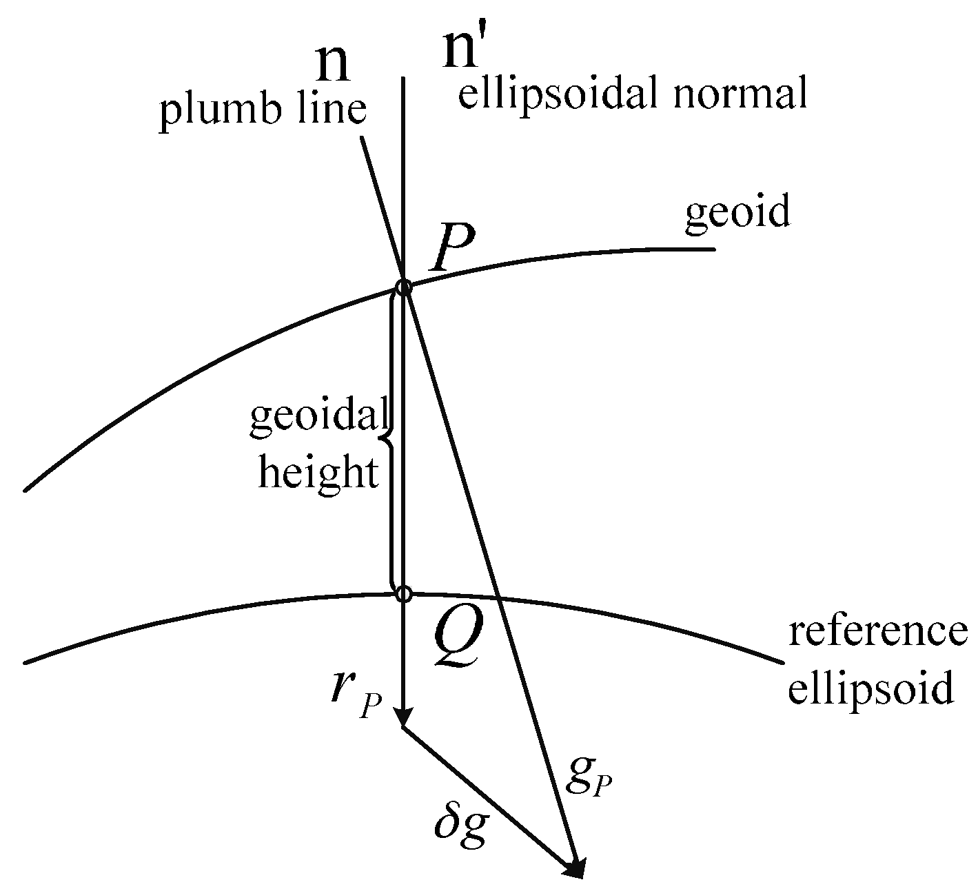
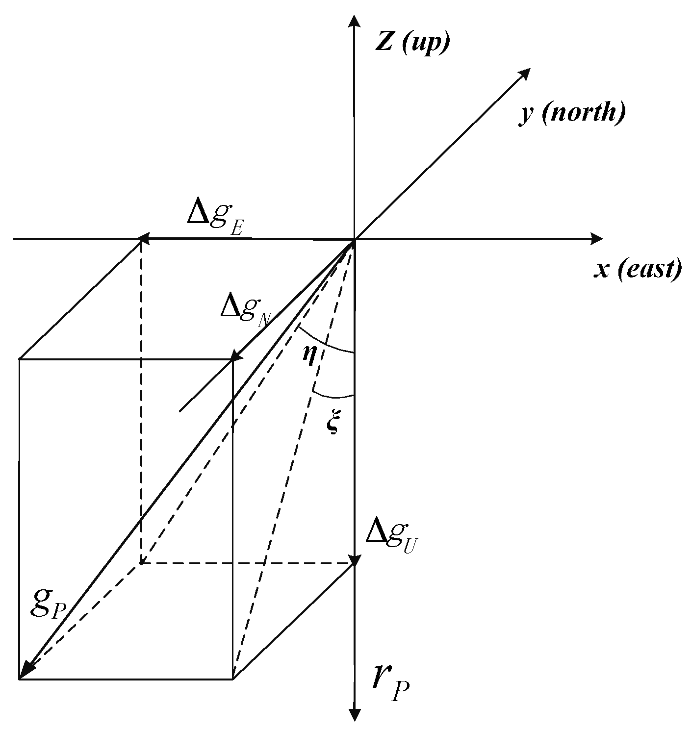
2.1. Definition of Gravity Disturbance Vector
2.2. INS Error Equations Considering Gravity Disturbance
3. Brief Review of Artificial Neural Networks
4. The Theory and Framework of the ELM-Based Gravity Disturbance Compensation Method in INS
- (1)
- No parameters need to be tuned except the predefined network structure;
- (2)
- ELM is capable of faster learning, and most trainings can be completed quickly;
- (3)
- ELM can achieve a high generalization performance;
- (4)
- ELM has a wide selection range of activation functions that are all piecewise continuous functions that can be used as activation functions.
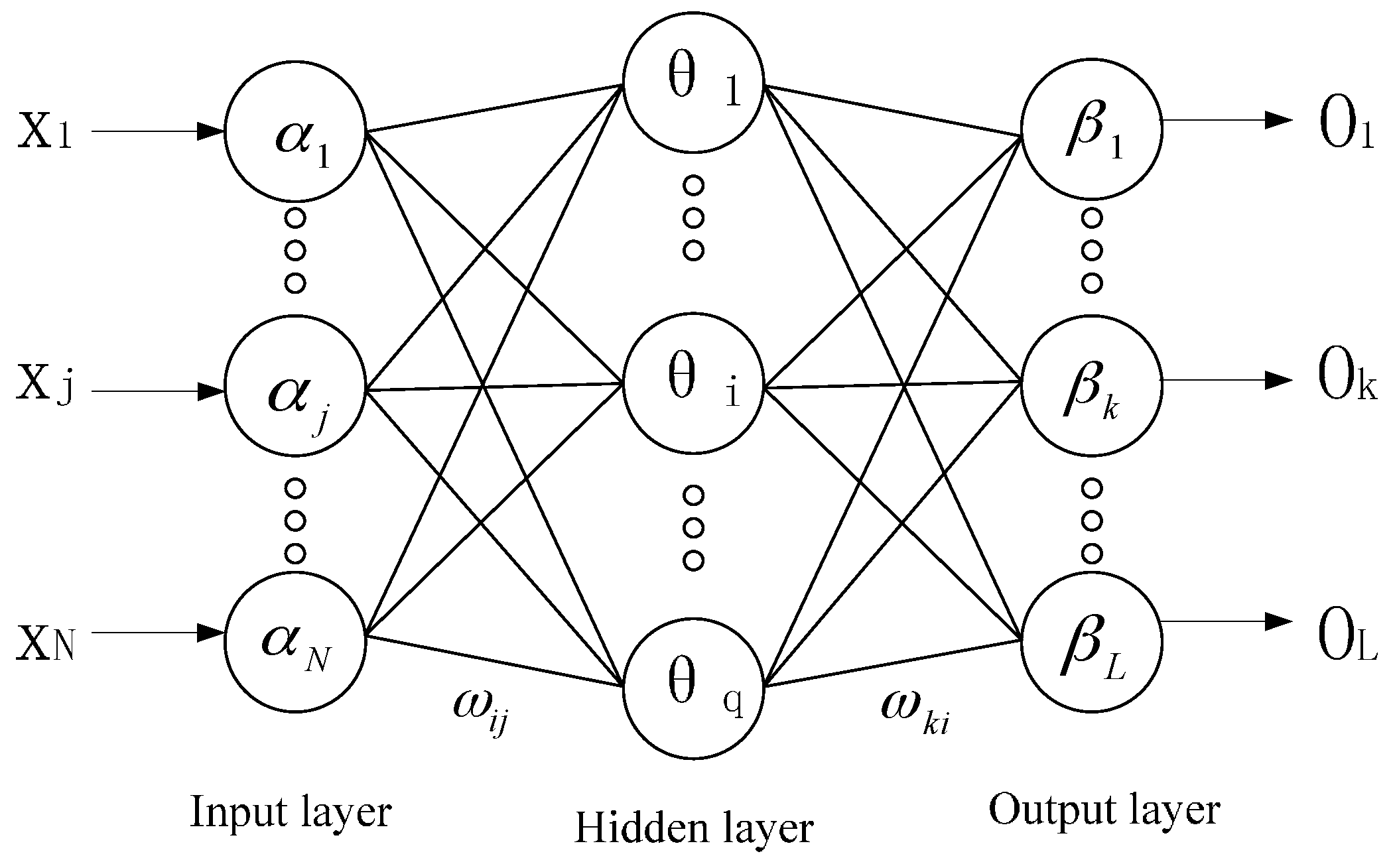
4.1. Extreme Learning Machine
| Algorithm 1. Extreme learning machine (ELM). |
| 1. Given a training set with N distinct examples , activation function g(x) and hidden neuron number ; |
| 2. Set input weights ω and hidden biases b from [–1,1] at random; |
| 3. Calculate the hidden layer output matrix H using matrix multiplication; |
| 4. Calculate the output weights according to the Moore–Penrose generalized inverse. |
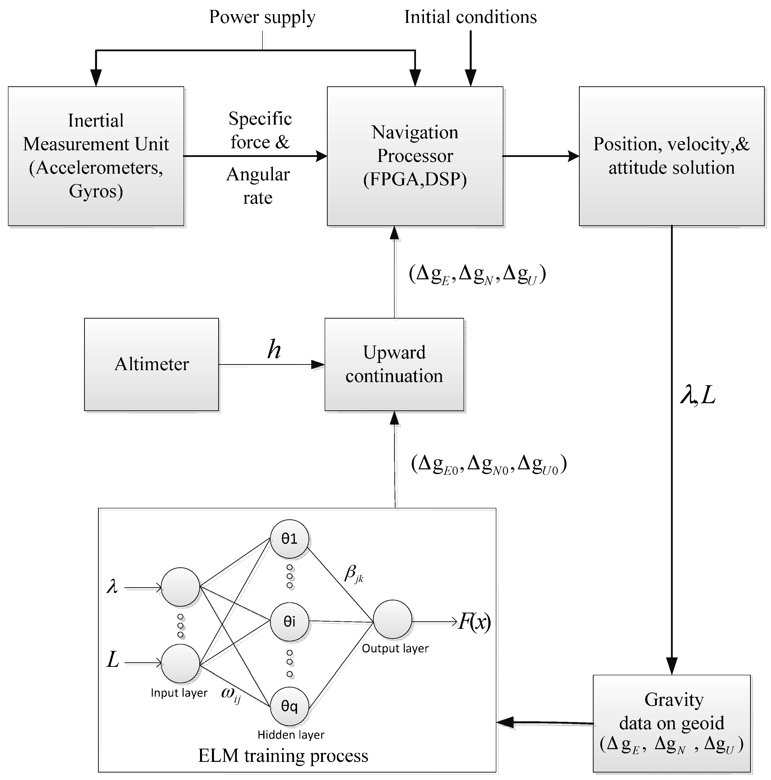
4.2. The Framework of the ELM-Based Gravity Compensation Method
- Get the INS position. Obtain the position value of the INS, longitude (λ) and latitude (L), through the calculation of INS.
- Choose the gravity database. Search the adaptive gravity database (provided by Institute of Geodesy and Geophysics, Chinese Academy of Sciences) according to the position obtained by Step 1. The gravity disturbance is related to the correlation distances. This means too wide a training area will not improve the estimation result, and too small a training area will not include enough information for the estimation of the gravity disturbance. After many trainings, we found that the size of the training area set as 5′ × 5′ would have the best estimation result. Therefore, here, the gravity database is set as 5′ × 5′ and takes the position of the INS as the central point.
- ELM training: Set λ, L as the inputs of the ELM algorithm, and obtain the gravity disturbance on the geoid () through the training with the gravity database obtained by Step 2.
- Upward continuation: Process the gravity disturbance with upward continuation to the height where the INS is. The height of the INS is obtained by the altimeter. In geographic engineering applications, the most practical upward continuation method is free air correction. The computational formula is described as follows [24]:where is the value of the gravity disturbance on the geoid, is the value of the gravity disturbance where the INS is and H is the height value between the geoid and INS.
- Compensate the gravity disturbance calculated by Step 4 in the INS error equations to restrain the error propagation caused by gravity disturbance.
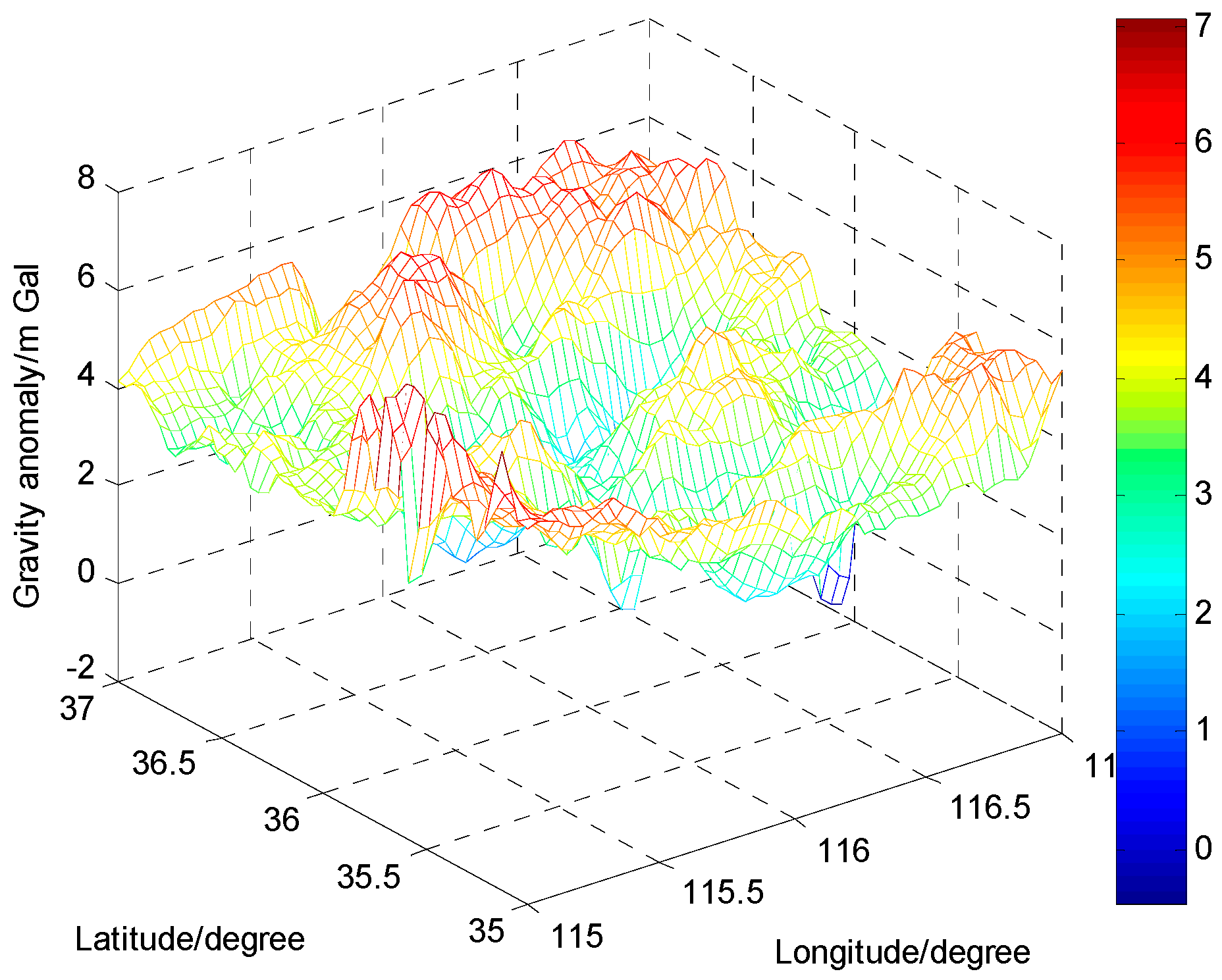
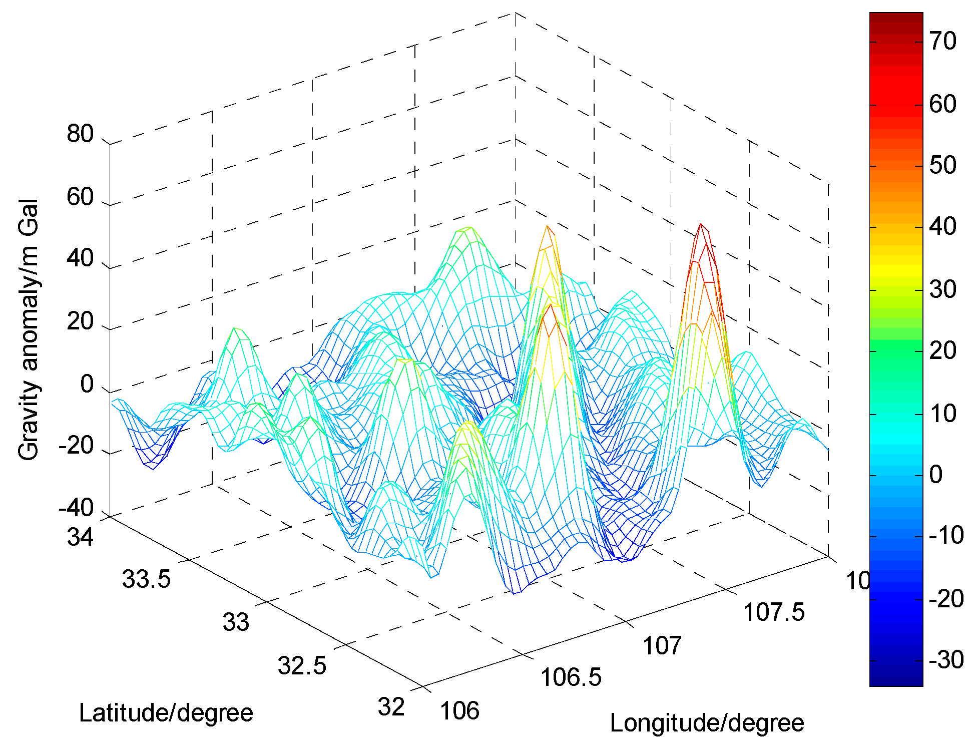
5. Numerical Test
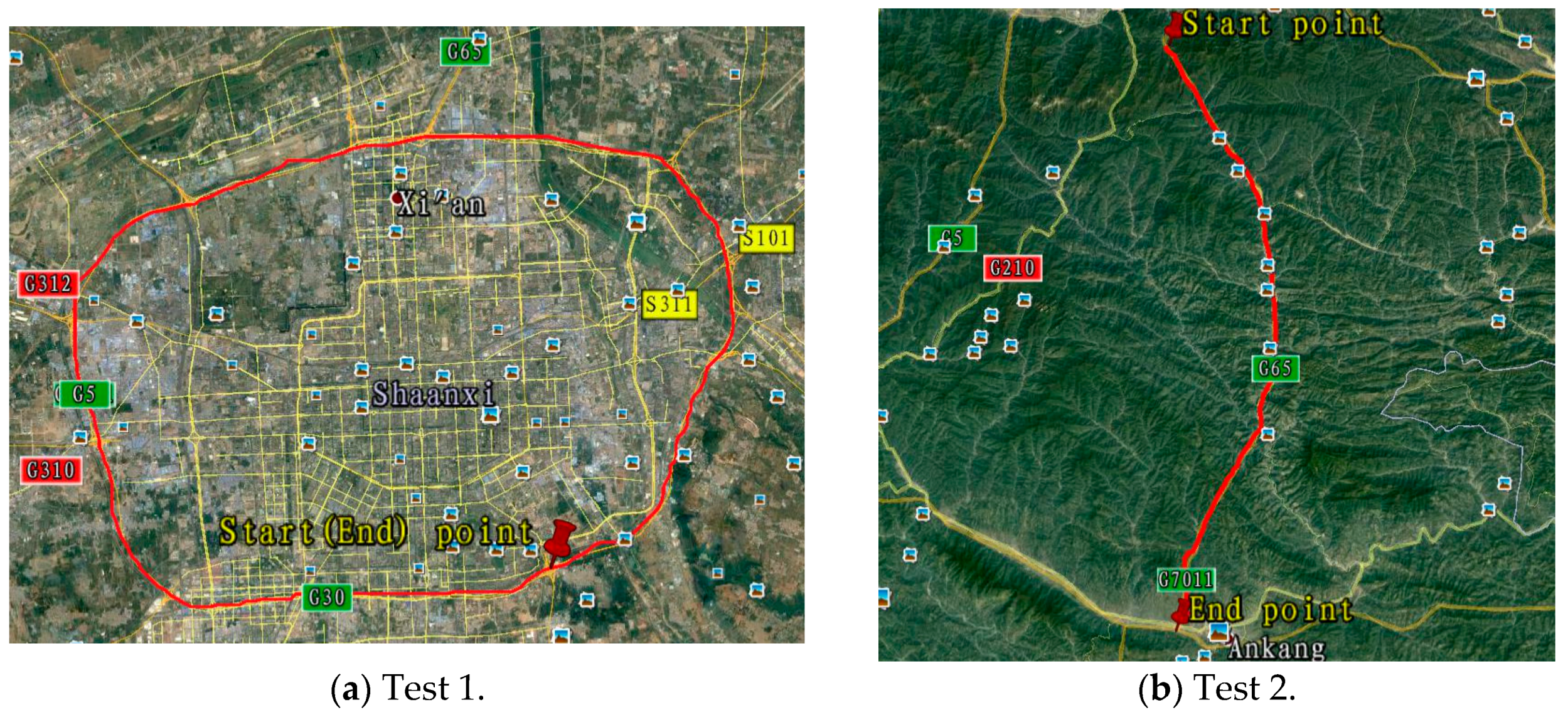
6. Experiment
7. Conclusions
Acknowledgments
Author Contributions
Conflicts of Interest
References
- Titterton, D.H.; Weston, J.L. Strapdown Inertial Navigation Technology, 2nd ed.; The Institution of Electrical Engineers: Stevenage, UK, 2004. [Google Scholar]
- Song, N.; Cai, Q.; Yang, G.; Yin, H. Analysis and calibration of the mounting errors between inertial measurement unit and turntable in dual-axis rotational inertial navigation system. Meas. Sci. Technol. 2013, 24, 115002. [Google Scholar] [CrossRef]
- Kwon, J.H.; Jekeli, C. Gravity requirements for ultra-precise inertial navigation. J. Navig. 2005, 58, 479–492. [Google Scholar] [CrossRef]
- Kwon, J.H. Gravity Compensation Methods for Precision INS. In Proceedings of the 60th Annual Meeting of the Institute of Navigation, Dayton, OH, USA, 7–9 June 2004.
- Jekeli, C. Precision free-inertial navigation with gravity compensation by an onboard gradiometer. J. Guid. Control Dyn. 2006, 29, 704–713. [Google Scholar] [CrossRef]
- Siouris, G.M. Gravity modeling in aerospace applications. Aerosp. Sci. Technol. 2009, 13, 301–315. [Google Scholar] [CrossRef]
- Mandour, I.M.; EI-Dakiky, M.M. Inertial Navigation System Synthesis Approach and Gravity-Induced Error Sensitivity. IEEE Trans. Aerosp. Electron. Syst. 1988, 24, 40–49. [Google Scholar] [CrossRef]
- Arora, N.; Russell, R.P. Fast efficient and adaptive interpolation of the geopotential. J. Guid. Control Dyn. 2014, 38, 1345–1355. [Google Scholar] [CrossRef]
- Heiskanen, W.A.; Moritz, H. Physical Geodesy, Reprinted at Institute of Physical Geodesy; Technical University Graz: Graz, Austria, 1996. [Google Scholar]
- Sarzeaud, O.; LeQuentrec-Lalancette, M.-F.; Rouxel, D. Optimal Interpolation of Gravity Maps Using a Modified Neural Network. Int. Assoc. Math. Geosci. 2009, 41, 379–395. [Google Scholar] [CrossRef]
- Huang, G.B.; Zhu, Q.Y.; Siew, C.K. Extreme learning machine: A new learning scheme of feedward neural networks. In Processing of the International Joint Conference on Neural Networks (IJCNN), Budapest, Hungary, 25–29 June 2004; pp. 985–990.
- Bazi, Y.; Alajlan, N.; Melgani, F.; AlHichri, H. Differential Evolution Extreme Learning Machine for the Classification of Hyperspectral Images. IEEE Geosci. Remote Sens. Lett. 2014, 11, 1066–1070. [Google Scholar] [CrossRef]
- Wang, D.D.; Wang, R.; Yan, H. Fast prediction of protein-protein interaction sites based on Extreme Learning Machines. Neurocomputing 2014, 77, 258–266. [Google Scholar] [CrossRef]
- Wellenhof, B.H.; Moritz, H. Physical Geodesy, 2nd ed.; Springer: Graz, Austria, 2005. [Google Scholar]
- Jordan, S.K. Effects of geodetic uncertainties on a damped inertial navigation system. IEEE Trans. Aerosp. Electron. Syst. 1973, AES-9, 741–752. [Google Scholar] [CrossRef]
- Harriman, D.W.; Harrison, J.C. Gravity-Induced Errors in Airborne Inertial Navigation. J. Guid. 1986, 9, 419–426. [Google Scholar]
- Li, H. Methods of Statistical Learning; Tsinghua University Press: Beijing, China, 2012; p. 143. (In Chinese) [Google Scholar]
- Zhou, Z.H.; Yang, Y.; Wu, X.D.; Kumar, V. The Top Ten Algorithms in Data Mining; CRC Press: New York, NY, USA, 2009; pp. 127–149. [Google Scholar]
- Wang, X.C.; Shi, F.; Yu, L. Analyses of 43 Cases of MATLAB Neural Network; Beihang University Press: Beijing, China, 2012. [Google Scholar]
- Huang, G.B.; Zhu, Q.Y.; Siew, C.K. Extreme Learning Machine: Theory and Applications. Neurocomputing 2006, 70, 489–501. [Google Scholar] [CrossRef]
- Huang, G.B.; Chena, L. Convex Incremental Extreme Learning Machine. Neurocomputing 2007, 70, 3056–3062. [Google Scholar] [CrossRef]
- Zhu, Q.Y.; Qin, A.K.; Suganthan, P.N.; Huang, G.B. Evolutionary extreme learning machine. Pattern Recognit. 2005, 38, 1759–1763. [Google Scholar] [CrossRef]
- Cao, J.W.; Lin, Z.P.; Huang, G.B. Self-Adative Evolutionary Extreme Learning Machine. Neural Process. Lett. 2012, 36, 285–305. [Google Scholar] [CrossRef]
- Lu, Z.L. Theory and Method of the Earth’s Gravity Field; Chinese People’s Liberation Army Publishing House: Beijing, China, 1996. [Google Scholar]
- GJB 729-1989. In The Means for Evaluation of Accuracy of Inertial Navigation Systems; Standards Press of China: Beijing, China, 1989. (In Chinese)
- Yang, G.L.; Wang, Y.Y.; Yang, S.J. Assessment approach for calculating transfer alignment accuracy of SINS on moving base. Measurement 2014, 52, 55–63. [Google Scholar] [CrossRef]


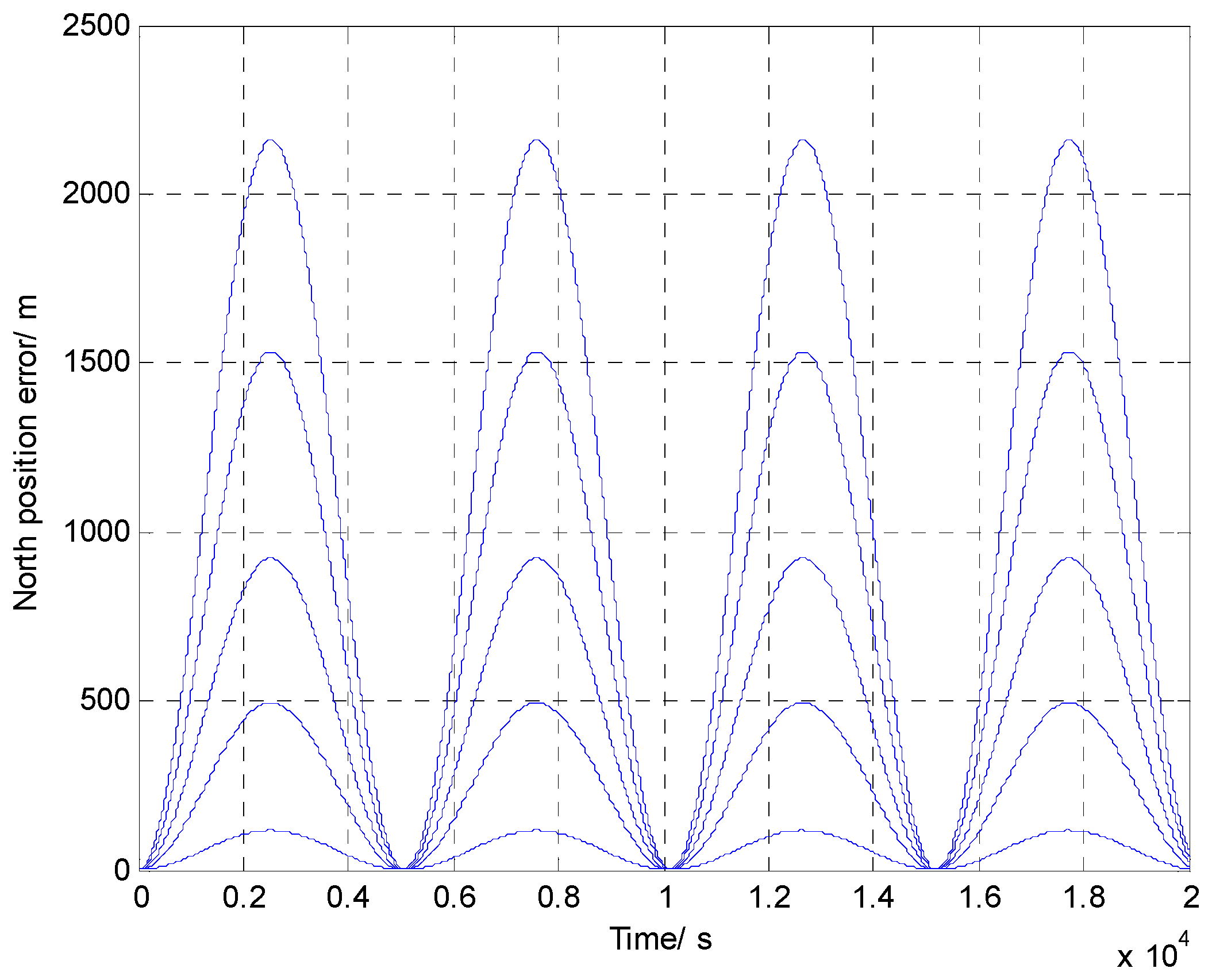
| = 2 s | = 8 s | = 15 s | = 25 s | = 35 s | |
|---|---|---|---|---|---|
| (m Gal *) | 9 | 38 | 71 | 118 | 166 |
| North position error (m) | 117 | 494 | 923 | 1534 | 2160 |
| Evaluation Criterion | Estimation Methods | ||
|---|---|---|---|
| IDW | Bilinear Interpolation | ELM | |
| MAE | 0.157 | 0.138 | 0.098 |
| MRE | 0.059 | 0.058 | 0.032 |
| RMSE | 0.285 | 0.279 | 0.213 |
| Evaluation Criterion | Estimation Methods | ||
|---|---|---|---|
| IDW | Bilinear Interpolation | ELM | |
| MAE | 0.228 | 0.203 | 0.128 |
| MRE | 0.076 | 0.056 | 0.041 |
| RMSE | 0.367 | 0.314 | 0.193 |
| Sensors Types | Characteristics | Magnitude (1 σ) |
|---|---|---|
| Gyroscope | Constant bias | 0.003°/h |
| Accelerometer | Constant bias | 10 μg |
| GPS velocity | Horizontal error | 0.03 m/s |
| Height error | 0.05 m/s | |
| GPS position | Horizontal error | 2 m |
| Height error | 5 m | |
| Altimeter | Measurement error | ±5 m |
| Measurement resolution | 0.1 m |
| Without Gravity Compensation | With Gravity Compensation | Position Improvement | |
|---|---|---|---|
| Test 1 | 1050 | 913 | 137 (13%) |
| Test 2 | 1120 | 790 | 330 (29%) |
© 2016 by the authors; licensee MDPI, Basel, Switzerland. This article is an open access article distributed under the terms and conditions of the Creative Commons Attribution (CC-BY) license (http://creativecommons.org/licenses/by/4.0/).
Share and Cite
Zhou, X.; Yang, G.; Cai, Q.; Wang, J. A Novel Gravity Compensation Method for High Precision Free-INS Based on “Extreme Learning Machine”. Sensors 2016, 16, 2019. https://doi.org/10.3390/s16122019
Zhou X, Yang G, Cai Q, Wang J. A Novel Gravity Compensation Method for High Precision Free-INS Based on “Extreme Learning Machine”. Sensors. 2016; 16(12):2019. https://doi.org/10.3390/s16122019
Chicago/Turabian StyleZhou, Xiao, Gongliu Yang, Qingzhong Cai, and Jing Wang. 2016. "A Novel Gravity Compensation Method for High Precision Free-INS Based on “Extreme Learning Machine”" Sensors 16, no. 12: 2019. https://doi.org/10.3390/s16122019