
Scalable Indoor Localization via Mobile Crowdsourcing and Gaussian Process

Abstract
:1. Introduction
- (1)
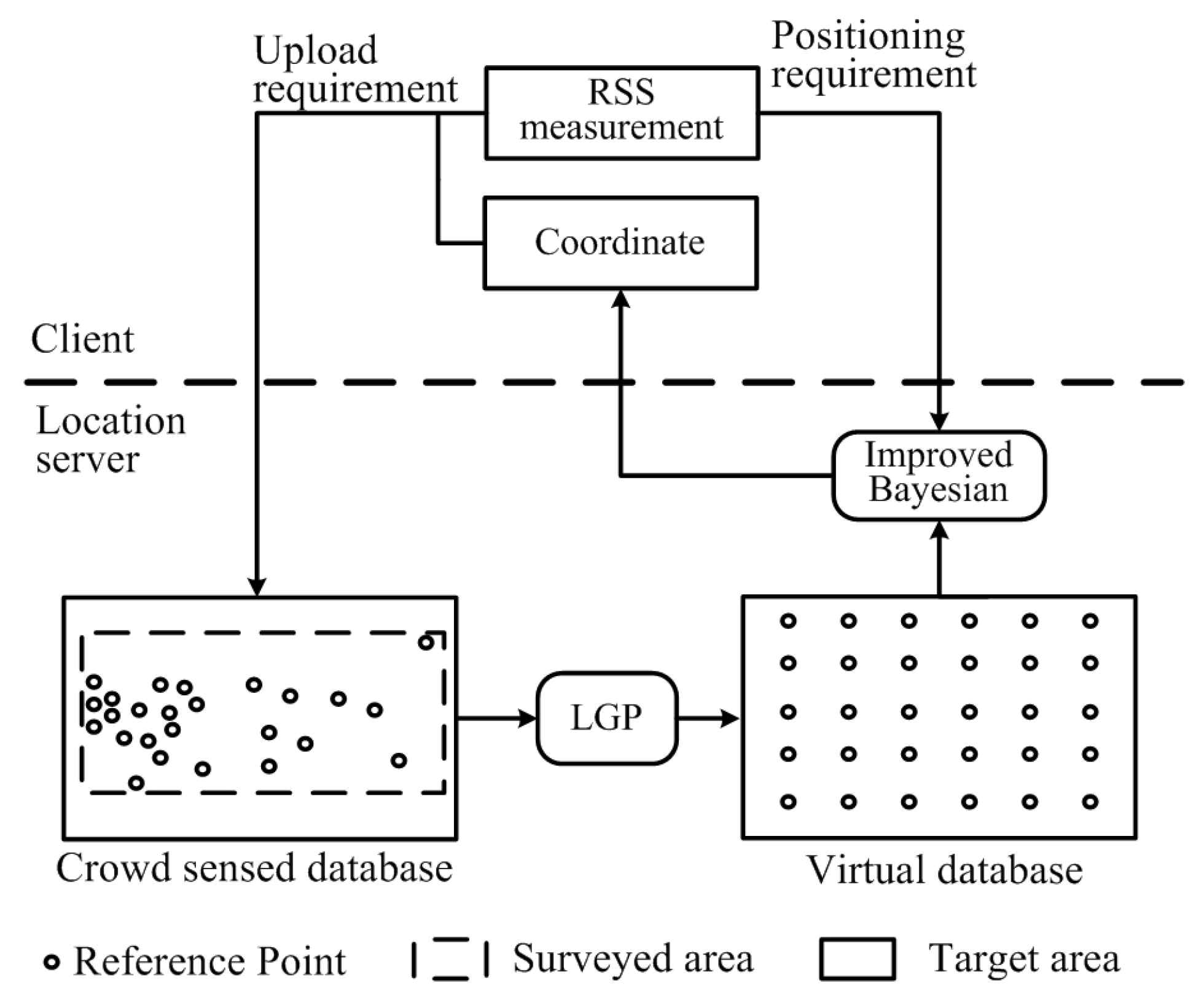
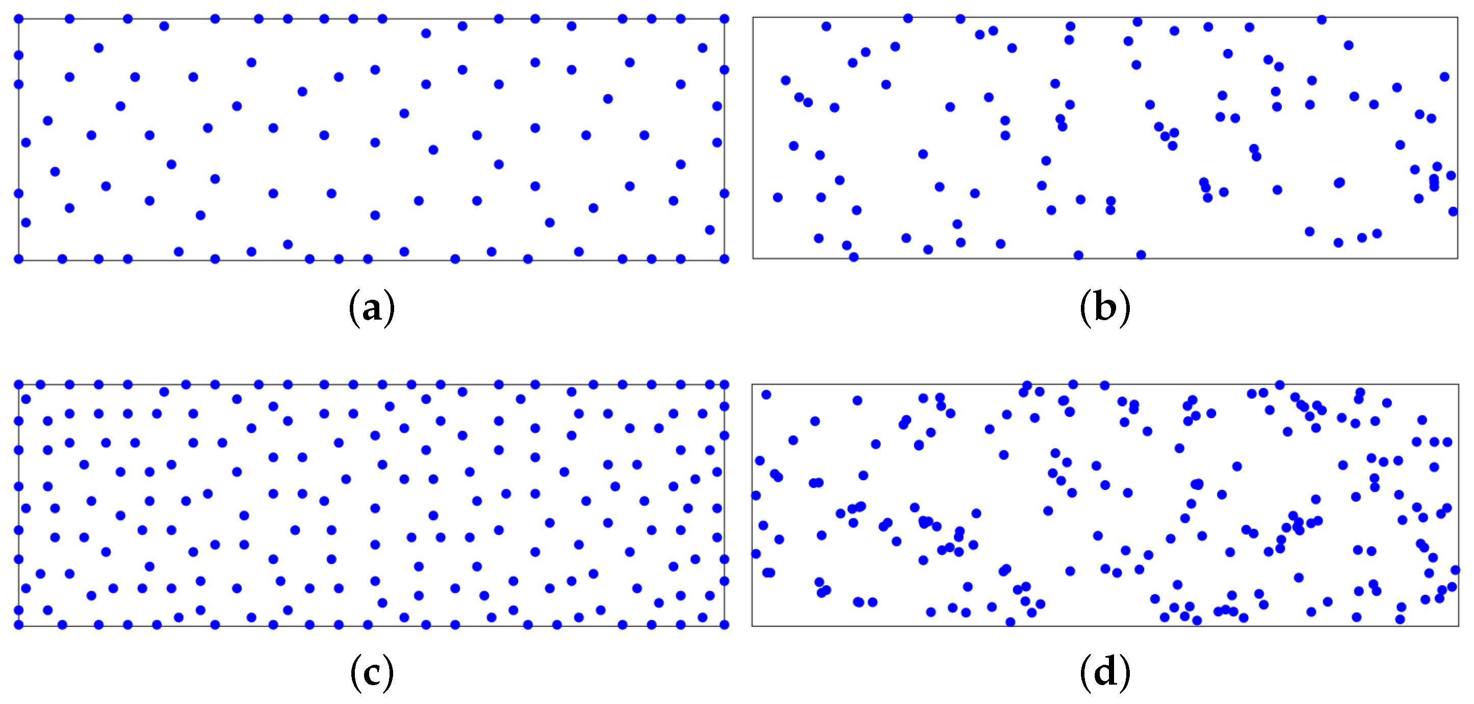
- We propose a MID algorithm to build a virtual database with uniformly distributed virtual RPs. The area covered by the virtual RPs can be larger than the surveyed area.
- (2)
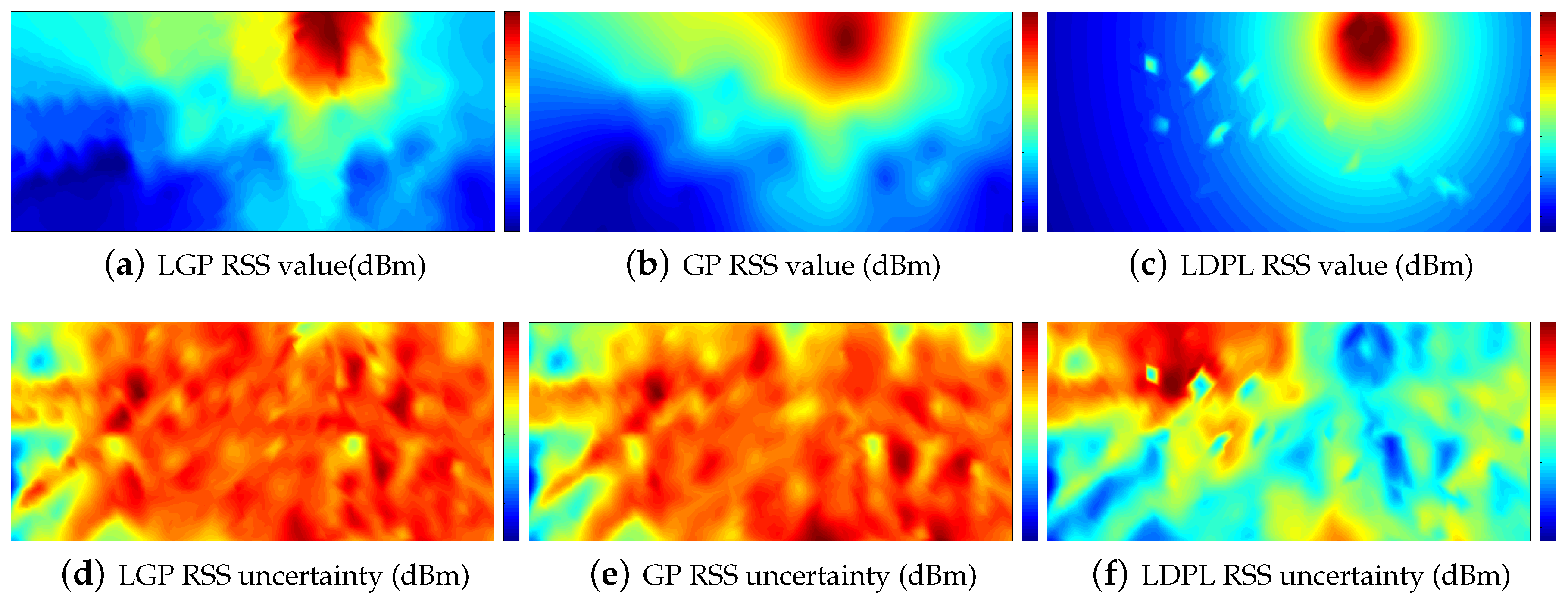
- The Local Gaussian Process (LGP) is applied to estimate the virtual RPs’ RSSI values based on the crowdsourced training data.
- (3)
- Bayesian algorithm is improved to estimate the user’s location using the virtual database.
- (4)
- We optimize all the parameters in the proposed algorithm by simulations.
- (5)
- An Android app is developed to test the proposed algorithm on real-case scenarios.
2. Related Works
3. Materials and Methods
3.1. Problem Setting and Algorithm Overview
3.2. Building the Dense Virtual Database
| Algorithm 1 |
| Require the target area P, the distance λ between neighbor virtual RPs in the number m of RPs we want to select. |
| Ensure select RPs every λ meters in P to build |
| Ensure randomly select from , |
| While() |
| For all() |
| Calculate using Equation (1) |
| End all |
| EndWhile |
3.3. Local Gaussian Process
3.4. Improved Bayesian Algorithm
4. Results and Discussion
4.1. Optimize the Parameters in the Algorithm
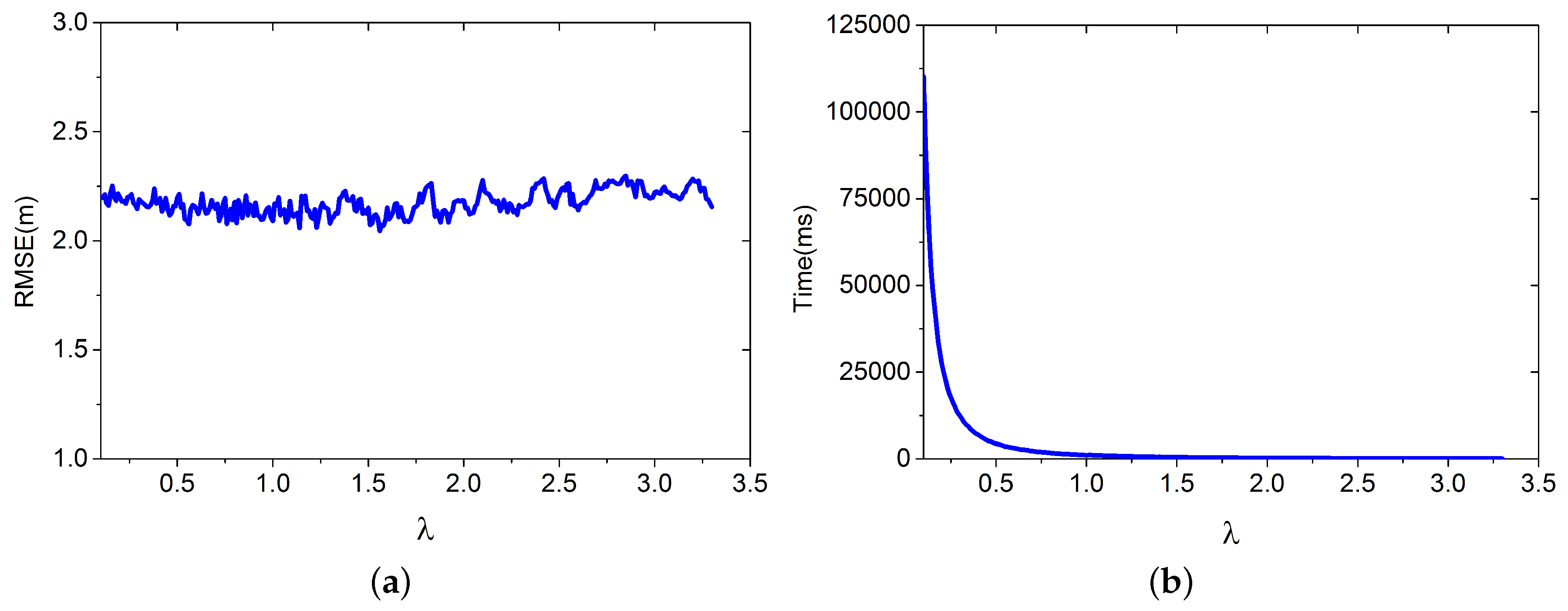
4.1.1. λ
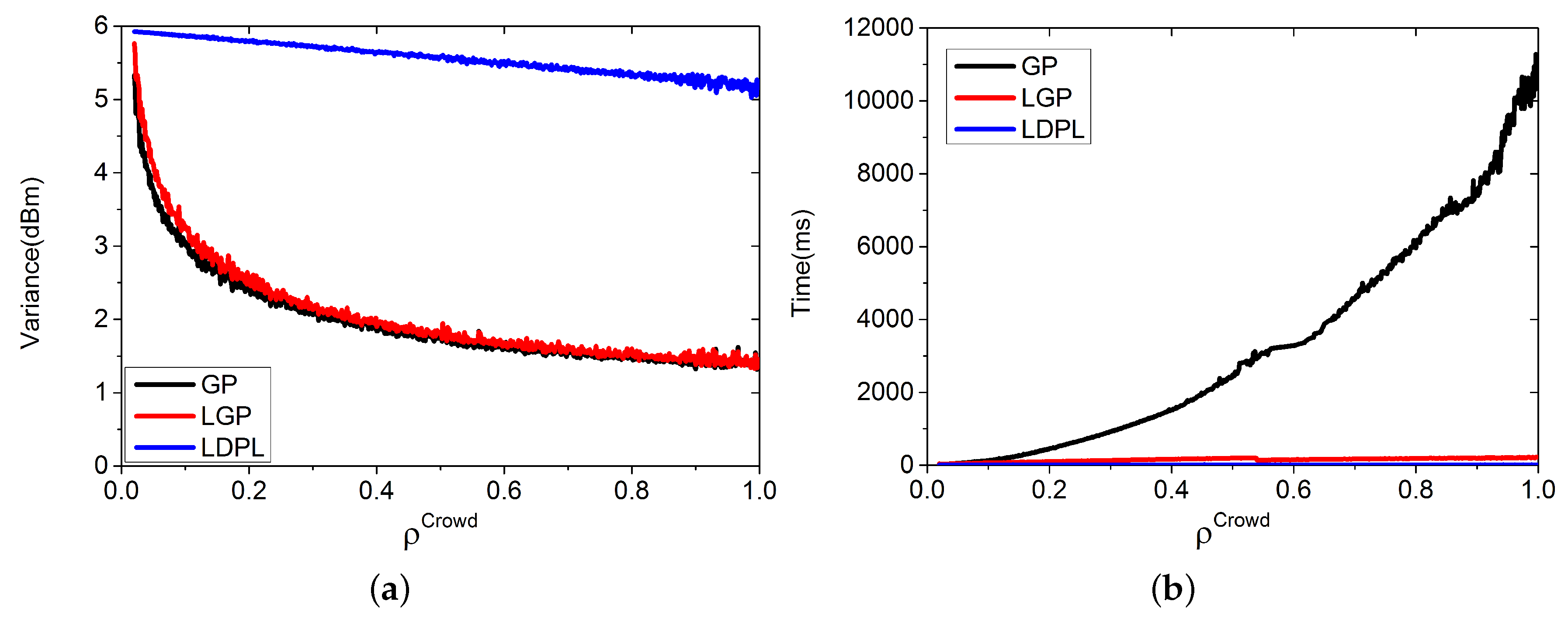
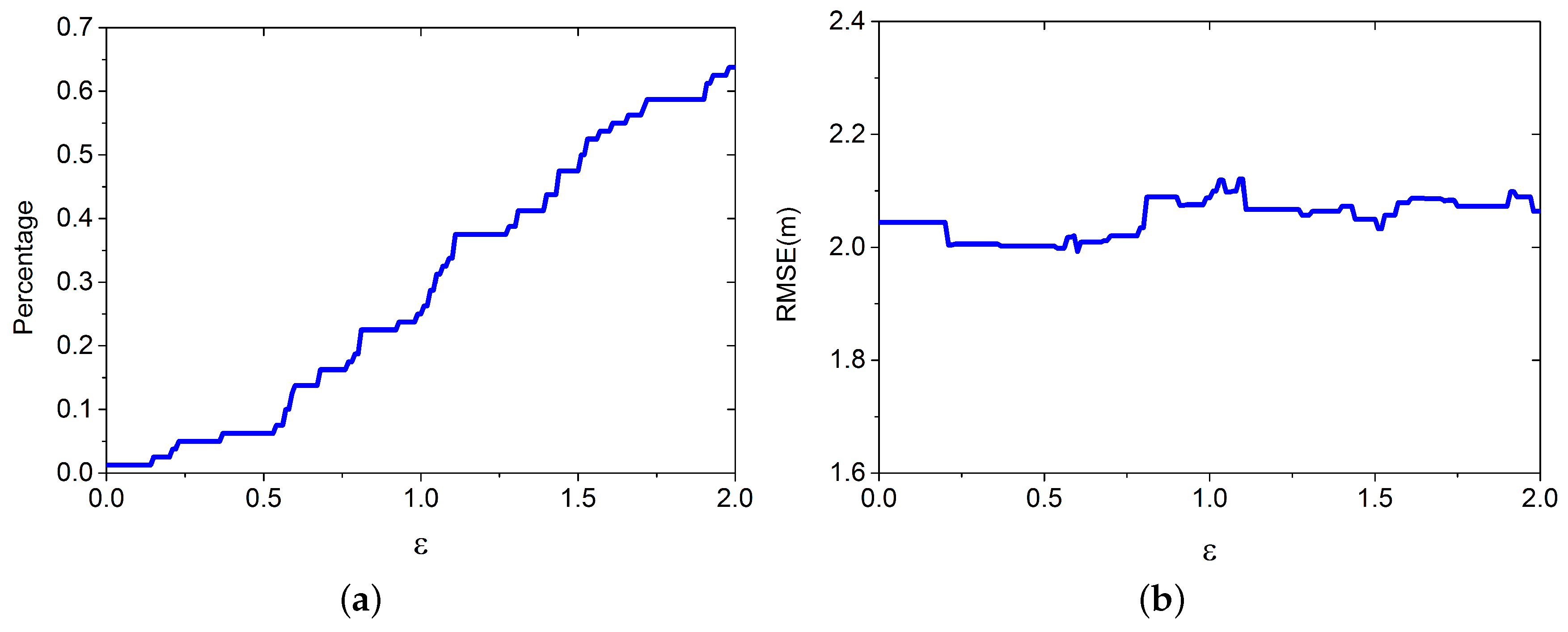
4.1.2. ε
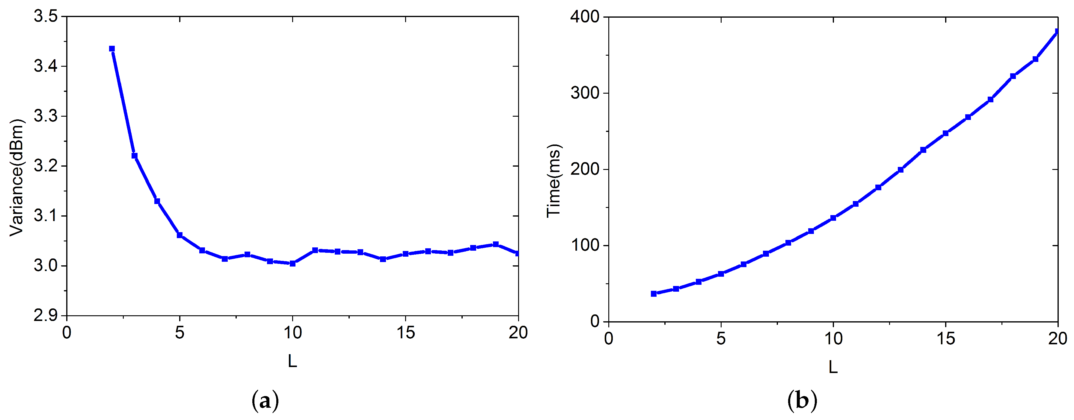
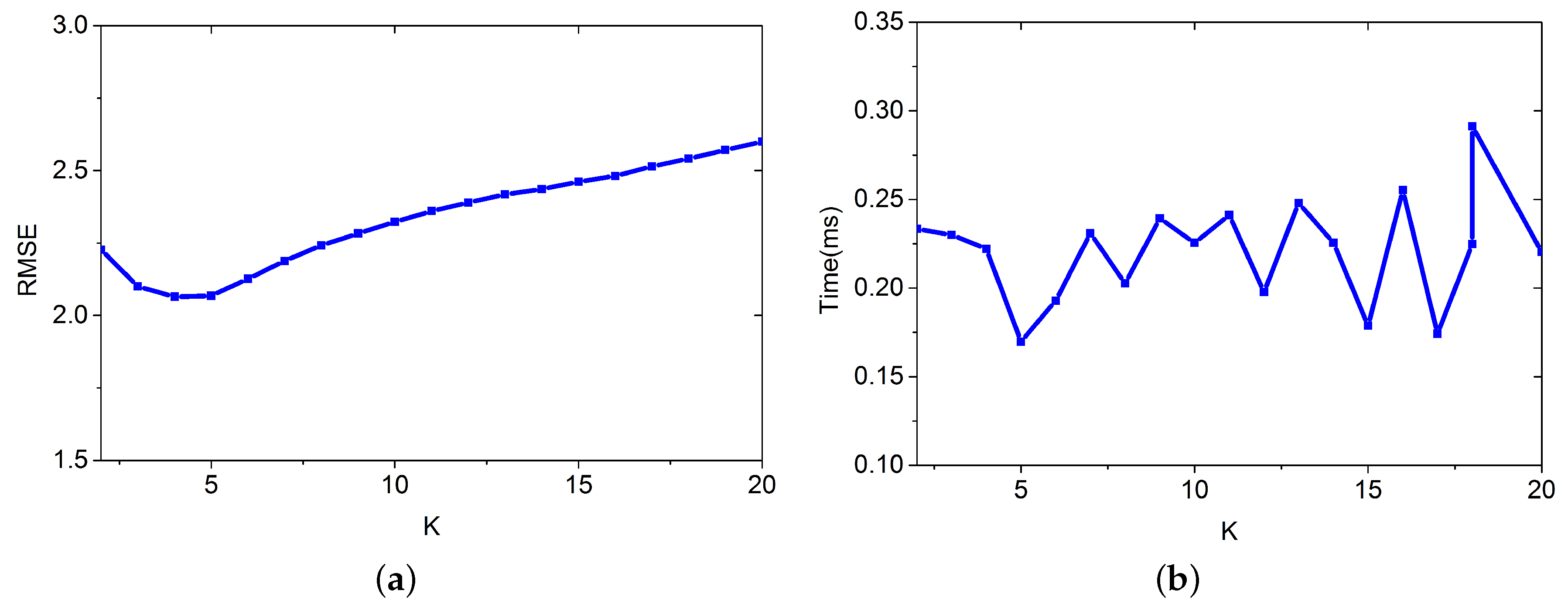
4.1.3. K
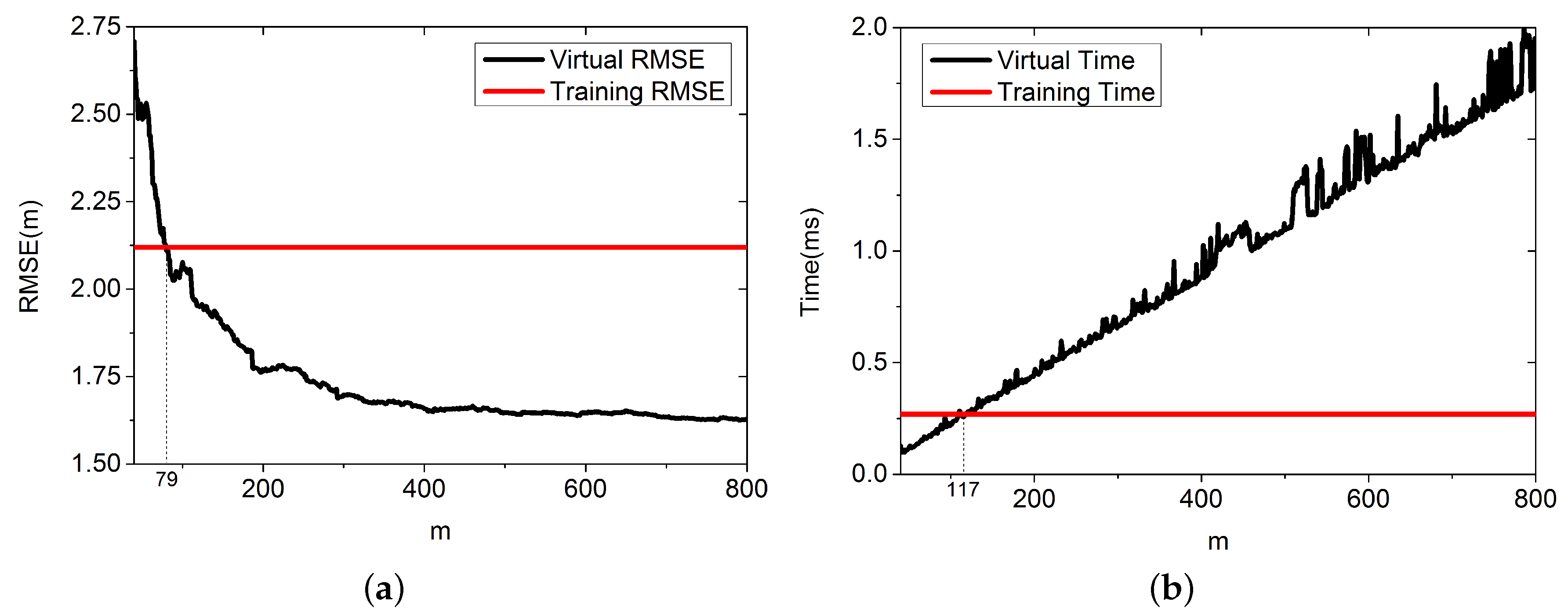
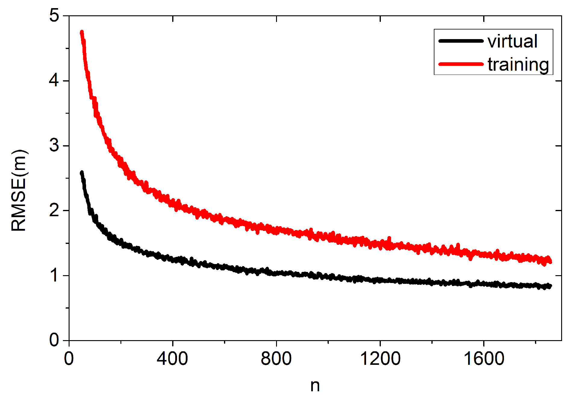
4.1.4. m
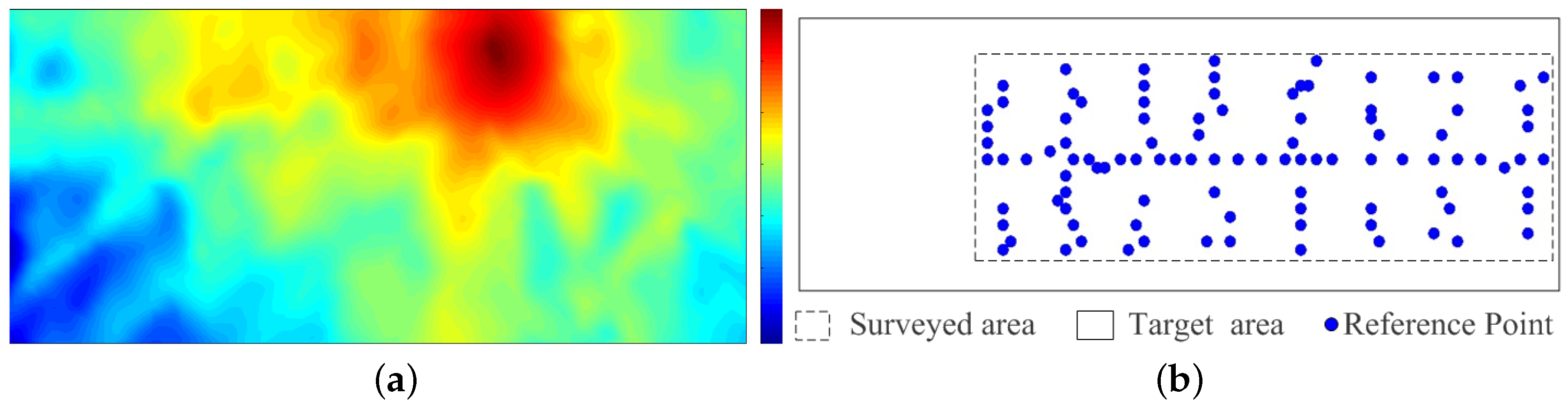
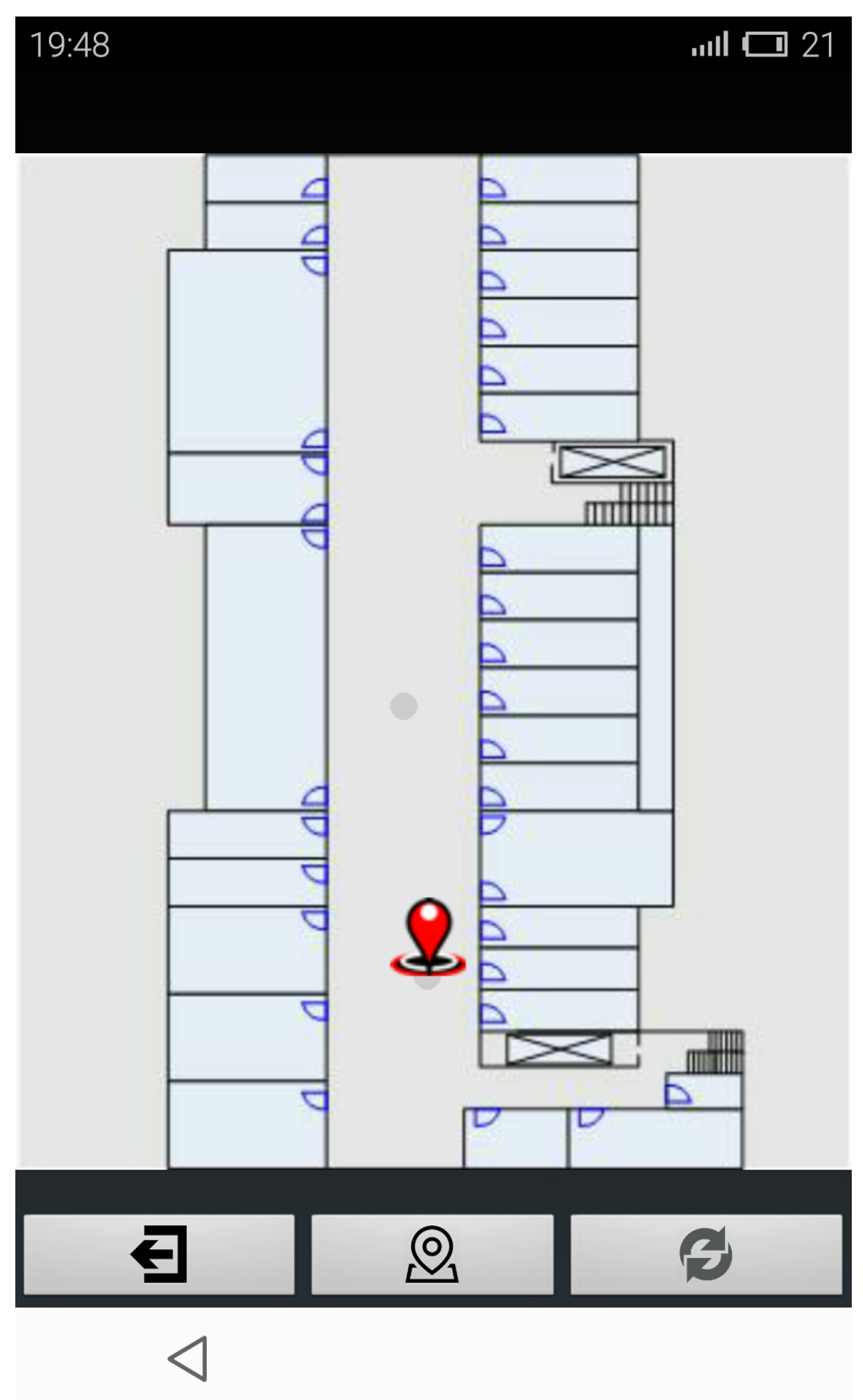
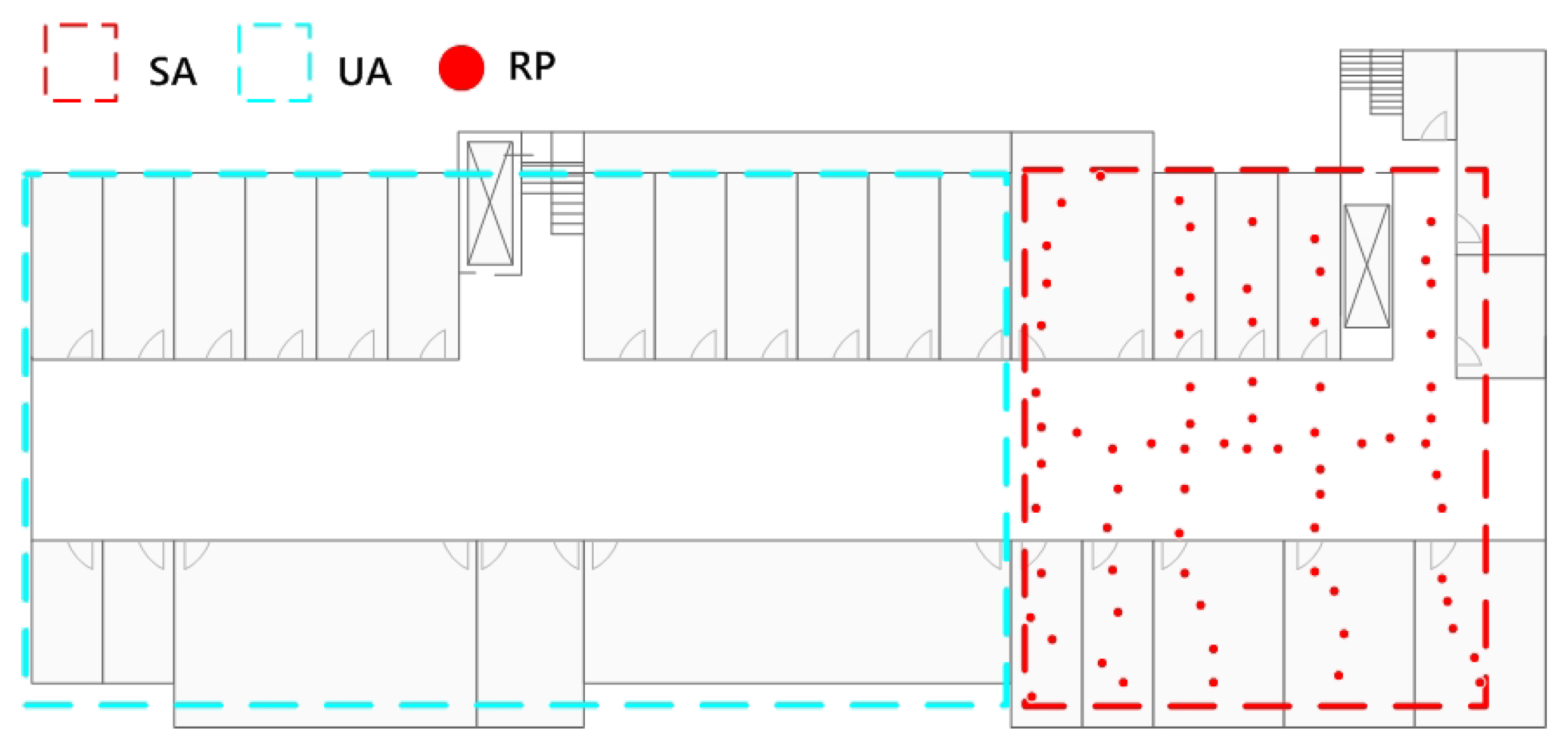
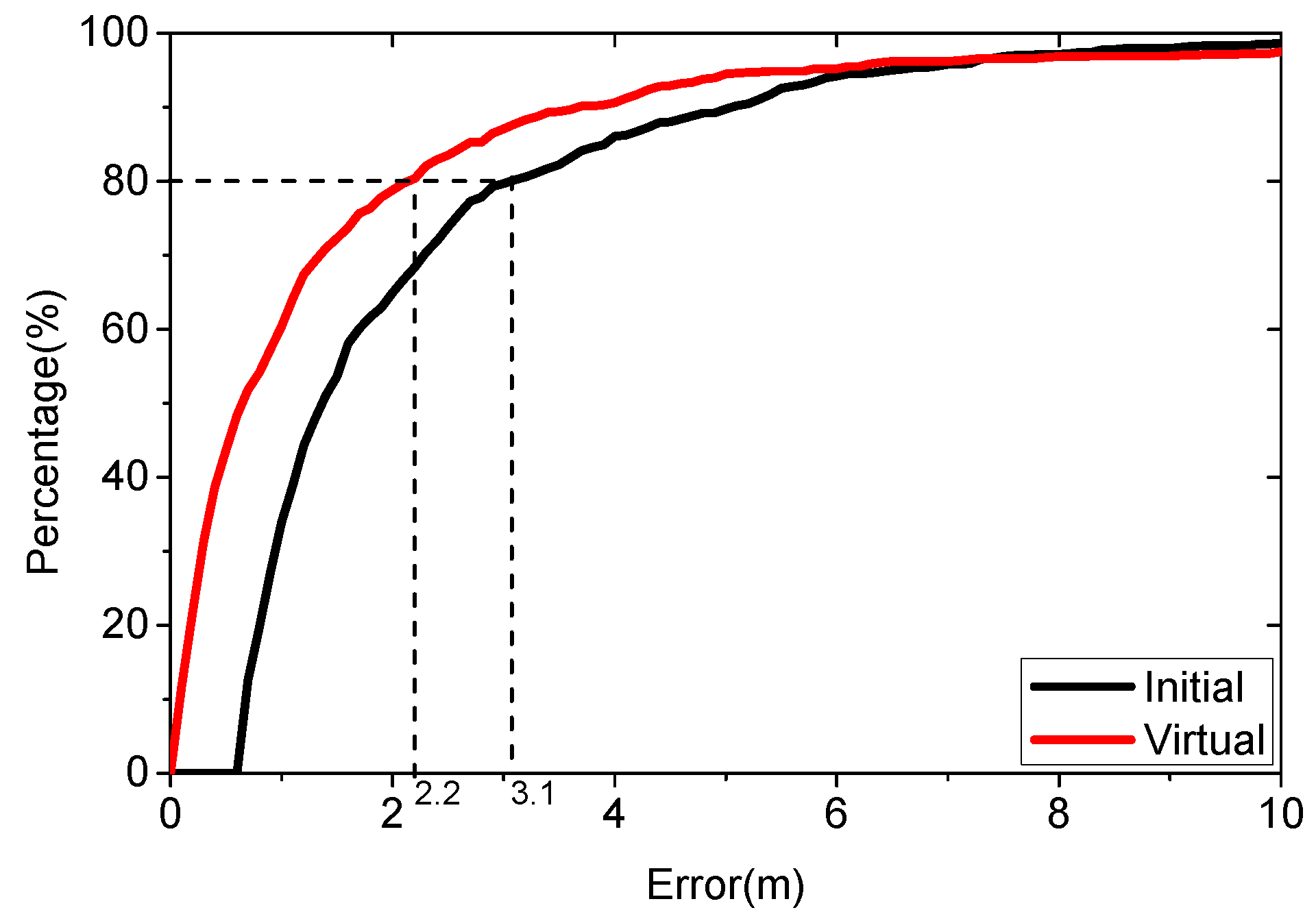
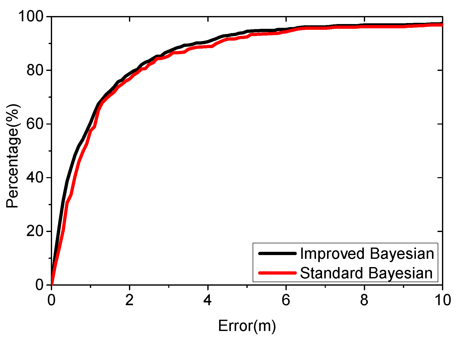
4.2. Real-Case Scenario Experiment
5. Conclusions
Acknowledgments
Author Contributions
Conflicts of Interest
References
- Gerstweiler, G.; Vonach, E.; Kaufmann, H. HyMoTrack: A Mobile AR Navigation System for Complex Indoor Environments. Sensors 2016, 16. [Google Scholar] [CrossRef] [PubMed]
- Bahl, P.; Padmanabhan, V.N. Radar: An in-building rf-based user location and tracking system. In Proceedings of the Nineteenth Annual Joint Conference of the IEEE Computer and Communications Societies (INFOCOM 2000), Tel Aviv, Israel, 26–30 March 2000; pp. 750–784.
- Guzman-Quiros, R.; Martinez-Sala, A.; Gomez-Tornero, J.L.; Garcia-Haro, J. Integration of Directional Antennas in an RSS Fingerprinting-Based Indoor Localization System. Sensors 2016, 16. [Google Scholar] [CrossRef] [PubMed]
- Google Maps, Google Maps Indoor. 2015. Available online: http://www.google.cn/maps/about/partners/indoormaps/ (accessed on 23 May 2015).
- Ferris, B.; Fox, D.; Lawrence, N. Wifi-slam using Gaussian process latent variable models. IJCAI 2007, 7, 2480–2485. [Google Scholar]
- Du, Y.; Yang, D.; Xiu, C. A Novel Method for Constructing a WIFI Positioning System with Efficient Manpower. Sensors 2015, 15, 8358–8381. [Google Scholar] [CrossRef] [PubMed]
- Bolliger, P. Redpin-adaptive, zero-configuration indoor localization through user collaboration. In Proceedings of the First ACM International Workshop on Mobile Entity Localization and Tracking in GPS-Less Environments, New York, NY, USA, 19 September 2008; pp. 55–60.
- Park, J.-G.; Charrow, B.; Curtis, D.; Battat, J.; Minkov, E.; Hicks, J.; Teller, S.; Ledlie, J. Growing an organic indoor location system. In Proceedings of the 8th International Conference on Mobile Systems, Applications, and Services, San Francisco, CA, USA, 15–18 June 2010; pp. 271–284.
- Rai, A.; Chintalapudi, K.K.; Padmanabhan, V.N.; Sen, R. Zee: Zeroeffort crowdsourcing for indoor localization. In Proceedings of the 18th Annual International Conference on Mobile Computing and Networking, Istanbul, Turkey, 22–26 August 2012; pp. 293–304.
- Yang, S.; Dessai, P.; Verma, M.; Gerla, M. Freeloc: Calibrationfree crowdsourced indoor localization. In Proceedings of IEEE INFOCOM, Turin, Italy, 14–19 April 2013; pp. 2481–2489.
- Wan, J.; Liu, J.; Shao, Z.; Vasilakos, A.V.; Imran, M.; Zhou, K. Mobile Crowd Sensing for Traffic Prediction in Internet of Vehicles. Sensors 2016, 16. [Google Scholar] [CrossRef] [PubMed]
- Chang, K.; Han, D. Crowdsourcing-based radio map update automation for Wi-Fi positioning systems. In Proceedings of the 3rd ACM SIGSPATIAL International Workshop on Crowdsourced and Volunteered Geographic Information, Dallas, TX, USA, 4–7 November 2014; pp. 24–31.
- Lee, M.; Yang, H.; Han, D.; Yu, C. Crowdsourced radiomap for room-level place recognition in urban environment. In Proceedings of the 2010 8th IEEE International Conference on Pervasive Computing and Communications Workshops (PERCOM Workshops), Mannheim, Germany, 29 March–2 April 2010; pp. 648–653.
- Wu, C.; Yang, Z.; Liu, Y. Smartphones based crowdsourcing for indoor localization. IEEE Trans. Mob. Comput. 2015, 14, 444–457. [Google Scholar] [CrossRef]
- Rappaport, T.S. Wireless Communications: Principles and Practice; Prentice Hall PTR: Lebanon, IN, USA, 2007. [Google Scholar]
- Kuo, S.-P.; Tseng, Y.-C. A scrambling method for fingerprint positioning based on temporal diversity and spatial dependency. IEEE Trans. Knowl. Data Eng. 2008, 20, 678–684. [Google Scholar]
- Barsocchi, P.; Lenzi, S.; Chessa, S.; Furfari, F. Automatic virtual calibration of range-based indoor localization systems. Wirel. Commun. Mob. Comput. 2012, 12, 1546–1557. [Google Scholar] [CrossRef]
- LaMarca, A.; Hightower, J.; Smith, I.; Consolvo, S. Self-mapping in 802.11 location systems. UbiComp 2005, 3660, 87–104. [Google Scholar]
- Maher, P.S.; Malaney, R.A. A novel fingerprint location method using ray-tracing. In Proceedings of the IEEE Global Telecommunications Conference (GLOBECOM 2009), Honolulu, HI, USA, 30 November 2009–4 December 2009; pp. 1–5.
- Raspopoulos, M.; Laoudias, C.; Kanaris, L.; Kokkinis, A.; Panayiotou, C.G.; Stavrou, S. 3D ray tracing for device-independent fingerprint-based positioning in wlans. In Proceedings of the 2012 9th Workshop on Positioning Navigation and Communication (WPNC), Dresden, Germany, 15–16 March 2012; pp. 109–113.
- Gomez, J.; Tayebi, A.; de Adana, F.M.S.; Gutierrez, O. Localization approach based on ray-tracing including the effect of human shadowing. Prog. Electromagn. Res. Lett. 2010, 15, 1–11. [Google Scholar] [CrossRef]
- Dissanayake, M.; Newman, P.; Clark, S.; Durrant-Whyte, H.F.; Csorba, M. A solution to the simultaneous localization and map building (slam) problem. IEEE Trans. Robot. Autom. 2001, 17, 229–241. [Google Scholar] [CrossRef]
- Choset, H.; Nagatani, K. Topological simultaneous localization and mapping (slam): Toward exact localization without explicit localization. IEEE Trans. Robot. Autom. 2001, 17, 125–137. [Google Scholar] [CrossRef]
- Koyuncu, H.; Yang, S.H. Indoor positioning with virtual fingerprint mapping by using linear and exponential taper functions. In Proceedings of the IEEE International Conference on Systems, Man, and Cybernetics (SMC), Manchester, UK, 13–16 October 2013; pp. 1052–1057.
- Keenan, J.; Motley, A. Radio coverage in buildings. Br. Telecom Technol. J. 1990, 8, 19–24. [Google Scholar]
- Pulkkinen, T.; Roos, T.; Myllymaki, P. Semi-supervised learning for wlan positioning. In Proceedings of the Artificial Neural Networks and Machine Learning-ICANN, Espoo, Finland, 14–17 June 2011; pp. 355–362.
- Varga, G.; Schulcz, R. Indoor radio location algorithm using empirical propagation models and probability distribution heuristics. Electr. Eng. 2013, 55, 87–96. [Google Scholar] [CrossRef]
- Li, L.; Shen, G.; Zhao, C.; Moscibroda, T.; Lin, J.-H.; Zhao, F. Experiencing and handling the diversity in data density and environmental locality in an indoor positioning service. In Proceedings of the 20th Annual International Conference on Mobile Computing and Networking, Maui, HI, USA, 7–11 September 2014; pp. 459–470.
- Rasmussen, C.E. Gaussian Processes for Machine Learning; MIT Press: Cambridge, MA, USA, 2006. [Google Scholar]
- Ferris, B.; Haehnel, D.; Fox, D. Gaussian processes for signal strength-based location estimation. In Proceedings of the Robotics Science and Systems, Philadelphia, PA, USA, 16–19 August 2006.
- Schwaighofer, A.; Grigoras, M.; Tresp, V.; Hoffmann, C. Gpps: A gaussian process positioning system for cellular networks. In Proceedings of the Neural Information Processing Systems, Lake Tahoe, NV, USA, 5–10 December 2013.
- Chiang, K.-W.; Liao, J.-K.; Tsai, G.-J.; Chang, H.-W. The Performance Analysis of the Map-Aided Fuzzy Decision Tree Based on the Pedestrian Dead Reckoning Algorithm in an Indoor Environment. Sensors 2016, 16. [Google Scholar] [CrossRef] [PubMed]
- Liu, Y.; Dashti, M.; Zhang, J. Indoor localization on mobile phone platforms using embedded inertial sensors. In Proceedings of the 10th Workshop on Positioning Navigation and Communication (WPNC), Dresden, Germany, 20–21 March 2013; pp. 1–5.
- Chai, W.; Chen, C.; Edwan, E.; Zhang, J.; Loffeld, O. 2D/3D indoor navigation based on multi-sensor assisted pedestrian navigation in wi-fi environments. In Proceedings of the Ubiquitous Positioning, Indoor Navigation, and Location Based Service (UPINLBS), Helsinki, Finland, 3–4 October 2012; pp. 1–7.
- AWE. Available online: http://www.awe-communications.com/ (accessed on 16 March 2015).
- Chintalapudi, K.; Iyer, A.P.; Padmanabhan, V.N. Indoor localization without the pain. In Proceedings of the sixteenth annual international conference on Mobile computing and networking, Chicago, IL, USA, 20–24 September 2010; pp. 173–184.
- Laoudias, C.; Zeinalipour-Yazti, D.; Panayiotou, C.G. Crowdsourced indoor localization for diverse devices through radiomap fusion. In Proceedings of the 2013 International Conference on Indoor Positioning and Indoor Navigation (IPIN), Montbeliard-Belfort, France, 28–31 October 2013; pp. 1–7.


| Algorithm | SA | UA | TA |
|---|---|---|---|
| GP | 1.86 | 8.09 | 5.77 |
| LGP | 1.88 | 8.25 | 5.88 |
| LDPL | 6.81 | 14.53 | 7.43 |
© 2016 by the authors; licensee MDPI, Basel, Switzerland. This article is an open access article distributed under the terms and conditions of the Creative Commons by Attribution (CC-BY) license (http://creativecommons.org/licenses/by/4.0/).
Share and Cite
Chang, Q.; Li, Q.; Shi, Z.; Chen, W.; Wang, W. Scalable Indoor Localization via Mobile Crowdsourcing and Gaussian Process. Sensors 2016, 16, 381. https://doi.org/10.3390/s16030381
Chang Q, Li Q, Shi Z, Chen W, Wang W. Scalable Indoor Localization via Mobile Crowdsourcing and Gaussian Process. Sensors. 2016; 16(3):381. https://doi.org/10.3390/s16030381
Chicago/Turabian StyleChang, Qiang, Qun Li, Zesen Shi, Wei Chen, and Weiping Wang. 2016. "Scalable Indoor Localization via Mobile Crowdsourcing and Gaussian Process" Sensors 16, no. 3: 381. https://doi.org/10.3390/s16030381