Article

Discrete Particle Swarm Optimization Routing Protocol for Wireless Sensor Networks with Multiple Mobile Sinks

1
School of Computer Science and Engineering, South China University of Technology, Guangzhou 510006, China
2
School of Medical Information and Engineering, Guangdong Pharmaceutical University, Guangzhou 510006, China
3
Data Analytics Department, Institute for Infocomm Research, 1 Fusionopolis Way, #21-01 Connexis (South Tower), Singapore 138632, Singapore
*
Author to whom correspondence should be addressed.
Sensors 2016, 16(7), 1081; https://doi.org/10.3390/s16071081
Submission received: 4 June 2016 / Revised: 6 July 2016 / Accepted: 8 July 2016 / Published: 14 July 2016
(This article belongs to the Special Issue New Paradigms in Cyber-Physical Social Sensing)

Abstract

:
Mobile sinks can achieve load-balancing and energy-consumption balancing across the wireless sensor networks (WSNs). However, the frequent change of the paths between source nodes and the sinks caused by sink mobility introduces significant overhead in terms of energy and packet delays. To enhance network performance of WSNs with mobile sinks (MWSNs), we present an efficient routing strategy, which is formulated as an optimization problem and employs the particle swarm optimization algorithm (PSO) to build the optimal routing paths. However, the conventional PSO is insufficient to solve discrete routing optimization problems. Therefore, a novel greedy discrete particle swarm optimization with memory (GMDPSO) is put forward to address this problem. In the GMDPSO, particle’s position and velocity of traditional PSO are redefined under discrete MWSNs scenario. Particle updating rule is also reconsidered based on the subnetwork topology of MWSNs. Besides, by improving the greedy forwarding routing, a greedy search strategy is designed to drive particles to find a better position quickly. Furthermore, searching history is memorized to accelerate convergence. Simulation results demonstrate that our new protocol significantly improves the robustness and adapts to rapid topological changes with multiple mobile sinks, while efficiently reducing the communication overhead and the energy consumption.

1. Introduction

Recently, wireless sensor networks (WSNs) have gained enormous attention for their wide range of applications [1]. WSNs consist of many tiny sensor nodes and one or multiple sinks, sensor nodes gather data from the sensing environment to sinks by communicating with each other. Energy efficiency is the most important issue in WSNs due to the limited battery capacity of sensor nodes. In WSNs with static sinks, the nodes close to the sinks would become hotspots and die earlier than others, because they are more likely to be the intersection of multihop routes and need to deplete their battery supplies to transmit huge amounts of data for other sensor nodes to the sinks [2]. Node death will result in a series of problems, such as disruptions in the topology, reduction of sensing coverage and packets loss, and so on. Therefore, routing protocols designed for WSNs have to incorporate load-balancing in order to achieve uniformity of energy consumption throughout the network. Mobile sinks are a good solution to avoid the hotspots [3,4]. In mobile based routing protocols, the hotspots around the sink change as the sink moves, which means that each node in the network has the chance to become the neighbor of the sink, so the high energy drainage around the sink is spread through the network, which helps achieving uniform energy consumption, and the network lifetime can be prolonged.
However, due to the sink mobility, the paths between source nodes and sinks are frequently updated, which introduces significant energy overhead. Therefore, mobile sink routing protocols should minimize the energy overhead of such operations while avoiding an extremely high increase of the sensor data delivery latency. A lot of distributed mobile sink protocols are proposed. Among these, the hierarchical protocols [2,5,6] are the most important and the most widely adopted, which aim to decrease the load of advertising the sink’s position to the network by constructing a virtual multitier (two or more) hierarchy role among the nodes. The high-tier nodes that can be easily reachable obtain and store the fresh sink position, while the remaining nodes query them to acquire the sink position whenever needed. Such a scheme does not need the network-wide sink advertisement, and thus significantly decreases the communication overhead and enhances the energy-efficiency of the network. However, the high-tier nodes may become hotspots. Yet the non-hierarchical protocols utilize mechanisms like flooding, overhearing or exploit geometric properties to advertise the sink’s position to the source nodes [7,8]. Thus, they can eliminate the overhead of constructing the virtual hierarchical structure and the possibility of hotspots on such a structure. However, they need the network-wide sink advertisement. The review of prominent hierarchical and non-hierarchical mobile sink routing protocols are presented in [9].
Recently, centralized nature-inspired algorithms have been studied to design routing protocol for MWSNs and have been proven to be good a solutions [10,11,12,13]. PSO is now prevailing due to its simple concept, easy implementation and effectiveness [14]; therefore, in this study, we employ PSO to build the optimal routing tree. In PSO-based protocols, routing establishment is formulated as an optimization problem; mobile sink masters the topology of the entire network by using network-wide flooding and runs various improved PSO to build the optimal routing paths for all source nodes. However, there are some shortages in existing schemes: (1) PSO is originally designed for continuous optimization problem, thus, they cannot deal with the discrete optimization problem as well as continuous optimization problems. Yet the routing optimization problem in MWSNs is discrete, and none of the existing solutions attempt to solve this problem. Therefore, the main goal of this paper is to propose a new discrete PSO algorithm by adapting the conventional PSO to build the optimal path tree more effectively in MWSNs; (2) Network-wide flooding significantly increased the communication overhead and energy consumption, while choosing the optimal routing result from all nodes greatly increases the computation burden. Thus, the second goal of this paper is to design a more efficient routing strategy; (3) As an evaluation criterion which helps us to periodically update the particles’ personal best position Pbest and the swarm’s global best position Gbest, fitness function is very important, because it directly affects the final results. Good fitness function improves the solution. In order to achieve better network performance, the existing fitness functions focus on maximizing the total remaining energy, and minimizing the total route length, total energy consumption and total communication delay of the candidate routing result. No attempt has considered such a case that the lifetime of a routing path just only depends on the relay node that has least lifetime, rather than the total remaining energy and total energy consumption. Therefore, the third goal of this paper is to give a better fitness function for our new routing protocol.
In this paper, we present an efficient routing strategy in which the greedy forwarding mechanism is employed as the underlying routing solution and the unicast local flooding method, rather than network-wide flooding, is adopted to reduce the communication and energy overhead caused by frequent broadcast communications. In our strategy, building routing tree from some source nodes to a mobile sink is formulated as an optimization problem, and the novel GMDPSO algorithm is put forward to solve this optimal problem. The main highlights of the proposed GMDPSO are as follows. First, we give a new fitness function in which we carefully calculated the energy consumption of relay nodes and try to minimize the distance among them to achieve energy conservation. Besides, we also minimize the total communication delay of routing tree. Second, the particle’s velocity and position of conventional PSO have been carefully redefined under discrete scenario so as to make them as easy as possible to encode/decode. Third, to effectively reduce the exhaustive global searching space and drive the particles to promising regions, the particle’s velocity and position updating principles have been thoroughly reconsidered by taking the advantage of the network topology of the collected candidate relay nodes by sink. Fourth, to avoid being trapped into local optima when building each optimal routing path, a greedy searching strategy specially designed for the particles to adjust their positions is proposed by improving the greedy forwarding mechanism. Fifth, searching history is memorized to accelerate convergence. By employing the provided GMDPSO and new fitness function, our new routing protocol is able to find the optimal routing tree, which well balances energy consumption of the relay nodes, delay and the overall rout tree length.
In summary, the contribution of this paper can be listed as follows.
  • An efficient routing strategy of the MWSNs is designed which is formulated as optimization problem.
  • A novel greedy discrete PSO with memory (GMDPSO) algorithm, which offers faster global convergence and higher solution quality, is put forward to quickly build the optimal routing tree, which can decrease the control overhead and minimize energy consumption.
  • Our new routing protocol is realized based on GMDPSO and more accurate new fitness function.
  • Simulations of the proposed protocol are performed to demonstrate its performance against some of the existing protocols.
The rest of the paper is organized as follows. The related work is presented in Section 2. Section 3 states the system model, which includes network model, energy model and fault model, and used terminologies. In Section 4, we present the routing strategy and the flowchart of our protocol. Section 5 gives a detailed description of the proposed GMDPSO, which is the core algorithm of our routing protocol. Section 6 evaluates the performance of our protocol by comparing it with other routing protocols. Finally, Section 7 concludes the paper.

2. Related Work

Various routing protocols have been proposed for MWSNs. TTDD (a Two-Tier Data Dissemination) [15] initially builds a rectangular grid structure which divides the network into cells with several dissemination nodes that are used to relay the query and data to/from the proper source. Whenever sinks request data, they query the network by local flooding within the cell and the query packets are relayed to the source nodes through dissemination nodes. A data path from the source to the sink is then established using the reverse of the path taken by the data request. However, TTDD suffers from the high overhead of constructing a separate grid for each source node. Unlike TTDD, Grid-Based Energy-Efficient Routing From Multiple Sources to Multiple Mobile Sinks (GBEER) [16] constructs a single combined rectangular grid structure for all possible sources to eliminate the high overhead of constructing separate grids for each source. However, the frequent grid change due to solving the hotspots introduces extra traffic on numerous nodes residing between the crossing points. In place of a rectangular grid, HPDD (Hexagonal Path Data Dissemination) [17] utilizes a common grid structure composed of hexagons. Which can provide shorter data and sink advertisement routes, but it suffers from the same hotspot problem. SEAD (Scalable Energy-efficient Asynchronous Dissemination) [18] constructs a minimum-cost weighted Steiner tree for the mobile sink by considering the distance and the packet traffic rate among nodes to save communication energy. Like TTDD, separate trees are constructed for each source; thus, the overhead of establishing such trees is very high. Ring Routing [19] designs an easily accessible ring structure to mitigate the anticipated hotspot problem with low overhead and minimize the data reporting delays. However, its questionable scalability is not good. Besides, the overhead of the initial ring construction for large or sparse networks will be high.
In agent-based schemes, one or more agents, which take on the role of representatives for the sources or the sink, are selected to relay the traffic between sources and the sink. These protocols usually utilize infrequent flooding to advertise the location of the agents. IAR (Intelligent Agent-Based Routing Protocol) [20] provides efficient data delivery to mobile sinks in large scale wireless sensor networks with sink mobility. IAR reduces the packet loss and signal overhead, meanwhile improves degraded route called triangular routing problem. However, as the hotspot, the agent (or IR) is chosen only depending on the distance to the sink without considering its remaining energy. Thus, once a node with low remaining energy is chosen to be the agent, it may die quickly, which leads to break the existing path to the sink. DHA (Data Dissemination Protocol Based on Home Agent and Access Node) [21] employs Home Agent and Access Node to design a simple protocol. Similar to IAR, the load on the home agent is immense, and changing the home agent requires global flooding. To decrease the frequency of global floods, SinkTrail [7] constructs and utilizes a logical coordinate space, which does not require position aware sensors and enables simple data dissemination by logical greedy geographic routing. However, the sink’s mobility is assumed to be nomadic and limits the applicability of the protocol. VGE-MGP [22] is another efficient mobile sink based routing without the physical geographic information.
Recently, nature-inspired algorithms are applied to solve the problem of the mobile based protocol. SIMPLE (swarm intelligence based protocol) [23] is based on a swarm agent that integrates the remaining energy of nodes into the route selection mechanism and maximizes the network’s lifetime by evenly balancing the remaining energy across nodes and minimizing the protocol overhead. The protocol is robust and scales well with both the network size and in the presence of multiple sinks. The movement of sinks may lead to the breakage of the existing routes. In most routing protocols, the query packets are broadcasted to repair a broken path from source node to sink, which causes significant communication overhead in terms of both energy and delay. In order to repair the broken path and maintain the available route from the source nodes to the mobile sink through a multi-hop network with lower communication overhead, IOLPSOR (immune orthogonal learning particle swarm optimization algorithm based routing recovery method) [11] is proposed to provide more efficient routing recovery capability to MWSNs. Furthermore, a more efficient ECPSOAR (efficient routing recovery protocol with endocrine cooperative particle swarm optimization algorithm) [10] is proposed to repair the broken path caused by both the movement of the sink and failure of sensor nodes. However, neither IOLPSOR nor ECPSOAR considers the following two cases. One case is that, the lifetime of the routing tree depends on the relay node that has the least lifetime. The other case is that, the improved PSOAs used by these two protocols do not well fit the discrete routing scenario.

3. System Mode and Terminologies

3.1. System Mode

We assume such a MWSN scenario: A wide open area is covered with a large number of homogeneous sensor nodes; there are N source nodes and M mobile sinks. Sinks can move anywhere within the sensor field, at any time with a fixed speed. Each source node sends its sensed data through multi-hops to the nearest sink via one and only one routing path. Several nodes can route packets to the mobile sink. In our network mode, individual node only owns the local information, such as its unique ID, residual energy level, delay and the distances to its neighbors, which can be estimated based on the received signal strength [24,25]. Our model does not need any extra positioning system such as GSP.
We use the same energy model and fault model proposed in [10]. The energy consumption equation of sensing and transferring m bit data is as follows:
Esens(m) = α1 × m
Etx(m, d) = (β1 + β2 × dis(i, j)n) × m
Erx(m) = γ1 × m
where dis (i, j) is the distance between n o d e   i and n o d e   j , Esens is the energy consumption of sensing m bits of data, Etx(m, d) and Erx(m) are the energy consumption of sending and receiving m bits of data, n is the channel attenuation index, α1, β1, β2 and γ1 are energy consumption parameters of sensing circuit, sending circuit, sending amplifier and receiving circuit, respectively. Let Pfault be the probability of sensor node’s failure in the network. We assume that the probability of the mobile sink failure is approximately 0. If any relay node is failed, it is handled by our routing algorithm.

3.2. Terminologies

Throughout this paper, we use the following terminologies:
  • S o u r c e j the jth sensor node. S i n k i is the ith mobile sink.
  • A g e n t i is the agent node belonging to S i n k i . One mobile sink has just only on agent node
  • N is the number of source nodes and M is the number of mobile sinks
  • R is the communication range of sensor node.
  • R N j k is the kth relay node on the path Pathj. R N j k + 1 is the next relay node of R N j k and   R N j k 1 is the previous relay node of R N j k .
  • N P a t h j   is the number of relay nodes in P a t h j . N P a t h S i n k i is the number of routing paths of   S i n k i .
  • P a t h j is the path from jth source node in the network to its nearest mobile sink S i n k i , P a t h j = {Sourcej, R N j 1 , R N j 2 , , R N j k , R N j N P a t h j , A g e n t i , S i n k i }.
  • P T r e e i is the routing tree of S i n k i .   P a t h j P T r e e i and R N j k P T r e e i .
  • l f ( R N j k ) means the lifetime of the R N j k . l f ( P T r e e i )   means the lifetime of the l f ( P T r e e i ) .
  • D e l a y ( R N j k ) is the delay of the R N j k . D e l a y ( P T r e e i ) means the overall delay of the P T r e e i .
  • Len( P a t h j ) means the length of the P a t h j . Len( P T r e e i ) means the overall length of the P T r e e i .
  • E c o n s ( R N j k ) is the energy consumed by R N j k due to data forwarding.
  • E c o n s P a t h ( P a t h j ) is the total energy consumption of routing path P a t h j .
  • G(V,E) or G means the connected graph containing all candidate relay nodes.
  • Set(V) is the set of all sensor nodes of G(V,E), i.e., the set of all candidate relay nodes.
  • NV is the number of sensor nodes in Set(V). N V   is the number of sensor nodes in Set(V) except the agent node,   N V = N 1 , i.e., the number of Set(V)-{ A g e n t i }.
  • Neig(nodei) is the set of all those sensor nodes within the communication range of nodei, therefore, Neig(nodei) = {nodej|0 < dis(nodei, nodej) ≤ R}.
  • NextRelay(noded) is the sensor node which is selected as the next relay node for noded. Therefore, NextRelay (noded) = {nodej|∀nodej dis(nodej, Agent) < dis(noded, Agent)}.

4. New Routing Protocol for MWSNs

In this section, we design an efficient routing strategy, based on the routing strategy, a new routing protocol is presented.

4.1. Our Efficient Routing Strategy in MWSNs

In our routing strategy, mobile sinks employ agent-based data gathering scheme [20,26,27] to collect sensed data. Our routing strategy can be described as follows.

4.1.1. Design of the Neighbor Table

Above of all, we design the neighbor table that is the key component of our protocol. It is illustrated in Table 1.
self_ID means a node itself, neighbor_ID means its neighbor node, Dis is the distance between seft_ID and neighbor_ID. isRelay is a Boolean flag indicating whether the node pair <self_ID→neighbor_ID > within a routing path, isRelay = 1 means true and data packet is routed from self_ID to neighbor_ID, its initial value is set to 0. Table 1 is the neighbor table for node 7 and illustrates that node 7 has two neighbor nodes: node 3 and node 9, the distance between node 7 and node 3 is 20, the distance between node 7 and node 9 is 15, in addition, <7→3> within a routing path.
Notably, our neighbor table is a wonderful issue. Some advantages can be summarized as follows: Firstly, neighbor table is the basic component of our protocol. Its basic function is used to record neighbor information which is the key information used to build the optimal routing path. Secondly, neighbor table enhances the MWSN scalability and the protocol robustness. When some nodes are failed, they will be deleted from its neighbors’ neighbor table on demand, and never be used to build the new optimal routing path. If the failed nodes are repaired or replaced, or new nodes are added in the MWSNs, corresponding neighbor information will be inserted into their neighbors’ neighbor table, thus, they can be used to build the new optimal routing path. Beyond that, when the routing path is changed, it is only to reset the isRelay flag of the relevant nodes, and this feature is well suited to resolve the routing problem in MWSNs. Thirdly, the isRelay flag indicates the routing information. It serves two purposes: routing tree establishment and locating the failed nodes. The routing tree is established by resetting the isRelay flag. In addition, if a relay node has not received any packet from its previous relay node after a reasonable time interval, it implies that the previous relay node has failed. With the help of the isRelay flag, the relay node can quickly find failed node ID from its neighbor table.

4.1.2. Building Routing Tree

Here, we detailed the procedure of building the routing tree from source nodes to sink. This procedure consists of the following steps:
Step 1 Network initiation and neighbor discovery. After all sensor nodes are deployed in the sensed field, all nodes can update their neighbor table using RSSI-based distant estimated scheme.
Step 2 Collect network statuses. When a sink move in a target area, the first thing has to be completed is to find the appropriate agent by local-broadcasting 1-hop Agent Query packet (AQ). The sink selected the closest node as the agent, and then broadcasts a Data Query (DQ) packet using unicast local flooding. Each node that receives the DQ packet firstly forwards the DQ to its neighbors and then updates its neighbor table if necessary. When a source matches DQ packet, it replies a Success Response (SR) packet to the sink. Each node that receives the SR packet firstly forwards the SR to its neighbors, then broadcast Data Query Response (DQR) packet that includes its newest state information such as residual energy, delay, and neighbor table data and so on along with its ID to the sink. Once the SR packet is received by sink, the data query procedure is finished immediately or finished after a reasonable time from then. This procedure as illustrates as Figure 1a. There are two special operations in this process are noteworthy. One is that all query packets (i.e., AQ and DQ) and their reply packets (i.e., DQR) are unicast by local flooding to reduce the overall communication and energy overhead. The other one is that, when a source node receivs multi DQ packets from multi sinks, it only replies to the first received DQ packet, which can assure it only sends its sense data to the nearest mobile sink to save energy.
Step 3 Build optimal routing tree. In most situations, multi-source nodes send data packets to a same sink, therefore, we need to build a routing tree. Root node is the agent, and the leaf nodes mean its source nodes. An example of routing tree is shown in Figure 2a. There are two routing paths, i.e., {Path1, Path2}, in the routing tree, the root node is Agenti and the leaf nodes are Source1 and Source2. The routing tree contains 5 relay nodes. Once finished Step 2. Sink has collected a number of neighbor tables along with their remaining energy information and delay information which are wrapped in DQR packets. As illustrated in Figure 1b, the network topology of candidate relay nodes that extracted from the neighbor tables, i.e., G(V, E), can be constructed by sink. Where eiE indicates that two adjacent sensor nodes can communicate with each other. G(V, E) is stored as adjacency matrix A, A[i, j] can be calculated as follows:
A [ i , j ] = { 0         i f    i = j   d i s ( i , j )    d i s ( i , j ) R         i f d i s ( i , j ) > R  
where i, j are two adjacent nodes, and dis(i, j) denote the length of eijE.
Each optimal routing path from each source node towards the sink can be built by using the improved greedy forwarding mechanism from candidates based on the network topology. Notably, even though each routing path (or branch) of a sink is optimal, the routing tree of the sink may not be the optimal due to the intersection relay nodes shared by multi paths. Therefore, the optimal algorithm needs to be employed to achieve the global optimum (the optimal routing tree). We designed GMDPSO , which is detailed in Section 5, to solve the problem.
Step 4 Establish routing tree and begin data transmission. After a mobile sink finished building the optimal routing tree in Step 3, it sends Routing Result (RR) packet, in which the routing tree can be stored as array, singly linked list or other forms, to its source nodes to establish the routing tree. The routing path establishment process can be detailed as follows: Assuming that Pathj = {Sourcej→11→9→7→3→ A g e n t i S i n k i } is a routing path of the routing tree.     S i n k i sends RR packet to its agent. When A g e n t i received the RR packet, it firstly search its previous relay node from the received packet according its ID, i.e., node 3. Then it sets isRelay = 1 for node pair { A g e n t i →node3} in its neighbor table. Next, A g e n t i replaces the destination address of RR packet with node3 and forwards it to node3. After received the RR packet, node 3 forwards it to its previous relay node7 as the same way, and so on for each relay node in the routing path. Finally, the source Sourcej received the RR packet, which means that the routing path is established completely and source can begin the data packet transmitting via the reverse path of RS packet towards source node. The detailed data forward process is described as follows: Sourcej generates a data packet and queries the neighbor_ID from its neighbor table as its next relay node using the condition isRelay = 1, i.e., node11, then the data packet is send to node11. After received the data packet, node 11 immediately queries its next relay node (i.e., node 9) and forwards data packet to node 9 in the same way, and so on for each relay node in the routing path. Finally, all data packets from Sourcej are received by A g e n t i , and then S i n k i receives data packet from A g e n t i directly.

4.1.3. Routing Path Recovery

When sink moves out of the radio rang of agent or relay node fails, the original routing path need to be recovered to continue the data gathering. The routing recover procedure is detailed in two cases:
(1)
When sink moves out of the radio rang of agent.
S i n k i cannot receive any packet from   A g e n t i , then it needs to select a new agent and build a new routing path to continue the data gathering. To ensure no previous data packet is lost, Temporary Agent node (TA) is introduced in our routing strategy. This routing recovery result is shown in Figure 2b. In order to help the sink to judge whether or not it is within the radio rang of an agent, the agent and relay nodes are required to send at least one packet to sink for a time interval T. Therefore, even though they have nothing to send, they also need to send a NULL packet to sink. Therefore, if not any packet has been received from A g e n t i for time interval T, S i n k i can knows that it moves away from   A g e n t i . To continue the data gathering, the following steps need to be completed:
  • Step 1 Select the TA.
Sink selects the closest node as the TA. If the sink moves faster, then TA is farther away from   A g e n t i ,which means that more relay nodes are required between TA and   A g e n t i .
  • Step 2 Build the temporary routing path
After TA is selected,   S i n k i sends Temporary Routing Path Setup (TRPS) packet to A g e n t i via TA. Once received the TRPS packet,   A g e n t i sends its cached data packets which come from source Sourcej to TA along the reverse path of TRPS packet, the reverse path is named Temporary Path (TP). Because some data packets will be lost after the sink moved away from A g e n t i and before TP is established, the A g e n t i needs to cache the data packets in this time interval to avoid data loss. Once the A g e n t i received the TRPS packet, these cached data packets are routed to TA via TP.
  • Step 3 Collect network statuses.
The procedure is the same to Step 2 in Section 4.1.2. The only difference is that the sink sends Routing Path Reset (RPRS) packet to source Sourcej to collect the newly network status information.
  • Step 4 Build optimal routing path.
As same as Step 3 in Section 4.1.2. The only difference is that the optimal routing tree is built for the nearest source nodes using those nodes whose response packet (RPRSR) are received by sink.
  • Step 5 Establish routing tree and begin data transmission.
The procedure is the same as Step 4 in Section 4.1.2.
  • Step 6 Clear original routing path.
Notably, when the new optimal routing path established, the original routing path is still work on. Before source node begin routing data packet via new optimal routing path, it sends Routing Path Clear (RPC) packet to TA along the original routing path and TP, each relay node on the path that received RPC packet will reset its isRelay = 0 to remove routing state information. Once the original routing path and TP is cleared, TA becomes the new agent A g e n t i .
(2)
When the relay node fails
Now we consider the relay node fault tolerant. This routing recovery procedure is shown in Figure 2c.
  • Step 1 Locate the failed node
When a relay node (e.g.,   R N j k ) in Pathj = {Sourcej,   R N j 1 ,     R N j 2 ,   ,   R N j k ,   R N j n ,   A g e n t i ,   S i n k i } has failed, e.g., exhausted its battery power, then Pathj is broken, its next relay node R N j k + 1 can realize this situation if it cannot receive any packet from R N j k for a predetermined time interval T. Once detecting routing path is broken, R N j k + 1 immediately queries its neighbor table to obtain the failure node ID (i.e., R N j k ) and sends a relay node failure (RNF) packet, which includes the failure node ID to A g e n t i via the original path. The relay node in the original path that received the RNF packet, e.g.,   R N j k + 2 , forward it to the next relay node ( R N j k + 3 ) and reset its isRelay = 0 to remove routing information.
  • Step 2 Build new routing path without failed node
After received the RNF packet, A g e n t i removes the failure node R N j k from the set of all candidates Set(V) and executes our new protocol to re-build new optimal routing path with Set(V)-{ R N j k }. The subsequent steps are the same as routing recover for mobile moves away the current agent, which are described in Section 4.1.2.

4.2. Overview of New Protocol

Based on our efficient routing strategy, a new centralized discrete PSO routing protocol is presented to solve the problem of routing in MWSNs.
The new protocol consists of two phases, the various steps are depicted in the flowchart as shown in Figure 3. When a mobile sink moves in the sense area, the routing tree from nearest source nodes towards it will be established in phase 1. When a mobile sink moves away its agent, or its relay node fails, its original routing path is recovered in phase 2. The detailed description can be seen in Section 4.1.
It can be seen from Figure 3 that the GMDSPO is the core algorithm of our new protocol, which is used to build the optimal tree from the nearest source nodes to the mobile sink in both phase 1 and phase 2.

5. The Proposed GMDPSO for Our Protocol

5.1. PSO

PSO is a population-based stochastic searching algorithm, which is inspired by social behavior of bird flocking and fish schooling. The easy implementation, concise framework and fast computational convergence make PSO a popular optimization technique for solving continuous optimization problems.
PSO works with a swarm of a predefined size (say N p ) of particles. Each particle has a position and a velocity vector. The position vector gives a complete candidate solution to the optimization problem, and the velocity vector denotes the position-changing tendency. Each particle is evaluated by a fitness function to judge the quality of the solution to the problem .To search for the optimal solution, a particle iteratively updates its flying velocity and current position according to its own flying experience, i.e., personal best called Pbesti and according to the other particles’ flying experiences, i.e., global best called Gbest.
In canonical PSO, a particle updates its position and velocity using the following simple rules:
V i ( t + 1 ) = w × V i ( t ) + c 1 × r 1 × ( P b e s t i X i ( t ) ) + c 2 × r 2 × ( G b e s t X i ( t ) )
X i ( t + 1 ) = X i ( t ) + V i ( t )
where Vi = { v i 1 , v i 2 , …, v i D } and Xi = { x i 1 , x i 2 , 1 I 3 , …, x i D } are the ith particle’s (say P i ) velocity and position vector. w is the inertial weight. t means the current iteration and t + 1 is the next itreration. c1 and c2 are acceleration factors term as cognitive and socail componeents. r1 and r2 are two different uniformly distributed random numbers in the range [0,1]. Pbesti = { p b e s t i 1 , p b e s t i 2 , p b e s t I 3 , …, p b e s t i D } is the personal best position of P i and Gbest = {gbest1, gbest1, …, gbestD} is the global best position of the whole swarm.
Conventional PSO was designed to optimize continuous problems. However, its fast convergence and easy implementation yet effectiveness have driven us to extend continuous PSO to solve the discrete routing optimization problem in MWSNs.

5.2. GMDPSO: Greedy Discrete PSO with Memory

The GMDPSO makes use of the network topology of candidate relay nodes to guide particle’s position and velocity updates. The greedy strategy originated from greedy forwarding mechanism is proposed to direct particles to move towards better position. Some small operators, such as position initialization and memory mechanism, are introduced to speed up convergence. This section will describe the proposed algorithm in detail. The whole framework of GMDPSO is given in Algorithm 1.
Algorithm 1 Framework of GMDPSO Algorithm
Parameters: particle swarm size Np, number of iterations Gen, inertia weight w, learning factors c1 and c2;
Input:
(1) adjacency matrix A for Sinki;
(2) the residual energy vector Eres = {Eres (1), Eres (1), …, Eres (N − 1)}
(3) the delay vector Del = {Del(1), Del(2), …, Del(N − 1)};
Output: Gbext.X: the routing result
Step 1: initialize Prev
Step 2: for i = 1 to Np do//Initialize the population
P[i]. X = initPathTree // seeing Section 5.2.3 for more information
Prev = PrevP[i].X If P[i].XPrev// memorize new position
P[i]. V = 0
Pbest[i] = P[i]
Calculate Fitness   P [ i ] .   f i t   //Using Equation (26)
end
Step 3: Gbest = {P[k]|Fitness(Pbest[k]) = min(Fitness(Pbest[i]))}//update Gbest
Step 4: While (!(Terminate))
for i = 1 to Np do
Update P[i]//carefully described in Section 5.2.4
Memorize new position: Prev = Prev ∪ new P[i].X If P[i]. XPrev
Calculate Fitness   P [ i ] .   f i t
Update the Pbesti Pbest[i].X = P[i].X if Pbest[i].fit > P[i]. fit
end
Update the Gbest: Gbest = Pbest[best]
end
Step 5: output G b e s t . X
It is worthy noted that the Prev variable is delicately designed in GMDPSO, it memorizes the search history to avoid the same position be updated more than once during the iterative process, and thus can avoid lots of reduplicative search and promote particle to find a better position faster. In other words, it can speed up the convergence of the algorithm. The function of Prev is called memory mechanism.
The positions are iteratively updated until the termination condition is satisfied. In our approach, there are two termination conditions: predefined iteration number and accuracy requirements. Once one of the two conditions is satisfied, the algorithm stops and the particle Gbest is found, Gbest.X represents the clustering result or routing result.

5.2.1. Fitness Function Derivation

Fitness function is an important issue because it directly affects the final results. Now, we construct our fitness function (fitness) to evaluate the individual particle of population, in GMDPSO, the optimal tree is built such that it minimizes the fitness value. We have three objectives when build the optimal routing tree for Sinki (i.e., PTreei): The first one is to maximize the lifetime of the routing tree to achieve energy-consumption balancing; The second one is to minimize the length of the routing tree to achieve energy conservation and enhance reliability; and the third one is to minimize the communication delay to enhance network throughout. In order to tune the three objectives to build optimal routing tree, we need to normalize the above three objectives and use the weight sum approach (WSA) [28] to construct our multi-objective fitness function fitness. Therefore, our fitness function depends on the following parameters:
(1)
Lifetime of relay node
Our first objective is to maximize the routing tree lifetime, which is defined as the time interval from the establishment of the routing tree till its first relay node dies (FND). This is possible if we can maximize the lifetime of relay node that has least lifetime. Let R N j k be the kth relay node on the Pathj. The lifetime of R N j k is defined as follows:
l f ( R N j k ) = E r e s ( R N j k ) / E c o n s ( R N j k )
where Eres( R N j k ) is the residual energy of relay node R N j k , and E c o n s ( R N j k ) is its consumed energy. It can be seen from Equation (7) that, even though R N j k keeps more Eres( R N j k ), it maybe die faster if its E c o n s ( R N j k ) is bigger than others at the same time.
Now, we begin the energy consumption analysis for relay node. R N j k must consume energy to forward the incoming data packets, which come from source node whose routing path to sink goes through it. Before calculating the routing energy consumption, it is needed to calculate the total number of incoming packets, which come from other relay node toward sink. Since multi routing paths may share some relay nodes, the number of incoming packets can be recursively calculated as follows:
N i n ( R N j k ) = { 0 i f   N e x t R e l a y ( R N l x ) R N j k ,   l 1 l N p a t h s i n k i , R N l x P a t h l   { N i n ( R N l x ) | N e x t R e l a y ( R N l x ) = R N j k } ,   o t h e r w i s e
The relay node R N j k will consume its energy to receive Nin( R N j k ) incoming packets and forward them. Therefore, the total data forwarding energy consumption of R N j k can be calculated as follows:
E c o n s ( R N j k ) = N i n ( R N j k ) × E R + N i n ( R N j k ) × E T ( R N j k , R N j k + 1 ) = N i n ( R N j k ) × ( E R + E T ( R N j k , R N j k + 1 ) ) = N i n ( R N j k ) × m × ( γ 1 + β 1 + β 2 × d i s ( R N j k , R N j k + 1 ) n )
where m is the size of data packet.
Let m i n L f P T r e e i     be the minimum lifetime of the routing tree PTreei. Therefore, our first objective is:
Objective   1 : Maximize  m i n L f P T r e e i = min { l f ( R N j k ) | R N j k P T r e e i }
Using Equation (9) to substitute the E c o n s ( R N j k ) in Equation (7), then,
l f ( R N j k ) = E r e s ( R N j k ) / E c o n s ( R N j k ) = E r e s ( R N j k ) / N i n ( R N j k ) × m × ( γ 1 + β 1 + β 2 × d i s ( R N j k , R N j k + 1 ) n )
It can be seen that, if Eres( R N j k ) and Nin( R N j k ) are fixed, then lf( R N j k ) is negatively correlated with dis( R N j k , R N j k + 1 ). Therefore, it can be deduced that relay node with minimum lifetime is the relay node with the longest transition distance. That is,
m i n L f P T r e e i = R N j k = arg   max d i s ( R N j k , R N j k + 1 )   | j , 1 j N p a t h s i n k i  and  k , 1 k N P a t h j
where argmaxf(x) returns the value of x that maximizes f(x).
Bigger m i n L f P T r e e i     means smaller fitness value. Therefore, fitness is inversely proportional to the m i n L f P T r e e i , i.e.,
f i t n e s s     1 / m i n L f P T r e e i  
where 0 < 1/ m i n L f P T r e e i   ≤ 1.
m i n L f P T r e e i   is used to avoid node with lower residual energy being selected as sharing relay node whose load burden is heavy.
(2)
Routing Path Length
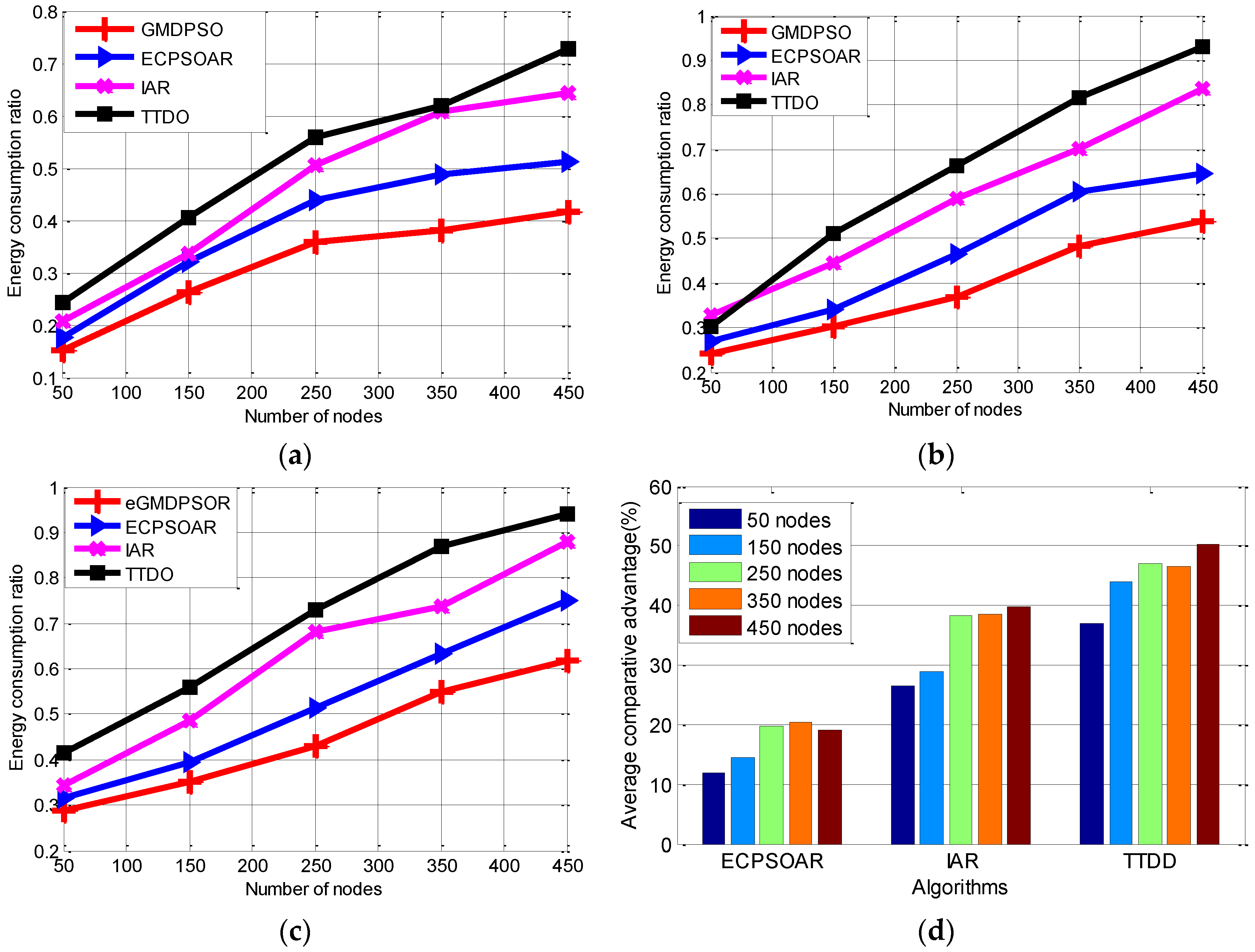
In our network mode, the energy is mainly consumed to collect network statuses and forward data to sink. The unicast local flooding mechanism is adopted to save energy for collecting network statuses. It is well known that the energy consumption of sensor node in WSNs is subject to the transmission distance—shorter data dissemination paths lead to decreased energy consumption together with increased throughput and reliability, which also can be deduced from Equation (9). Therefore, our second objective is to minimize the length of the routing tree to minimize the forwarding data energy consumption. Let P a t h j   be routing tree of A g e n t i . Now, we calculate the total energy consumption of PTreei (i.e., E c o n s P T r e e i ). According to Equation (9), the energy consumption of each routing path P a t h j ( P a t h j P T r e e i ), i.e., E c o n s P a t h j   , can be calculated as follows:
E c o n s P a t h j = k = 1 N P a t h j E c o n s ( R N j k ) = k = 1 N P a t h j N i n d a t a ( R N j k ) × m × ( γ 1 + β 1 + β 2 × d i s ( R N j k , R N j k + 1 ) n ) = k = 1 N P a t h j N i n ( R N j k ) × m × ( γ 1 + β 1 ) + β 2 × k = 1 N P a t h j d i s ( R N j k , R N j k + 1 ) n
Therefore, E c o n s P T r e e i can be calculated as follow:
E c o n s P T r e e i = j = 1 N p a t h s i n k i E c o n s P a t h j = j = 1 N p a t h s i n k i k = 1 N P a t h j N i n d a t a ( R N j k ) × m × ( γ 1 + β 1 ) + β 2 × j = 1 N p a t h s i n k i k = 1 N P a t h j d i s ( R N j k , R N j k + 1 ) n
For each Pathj assume that no packet is lost during routing data to agent, then Nin( R N j k ) is the same for each relay node in Pathj which can be considered as a constant value. Let Nin( R N j k ) = Nin. Then Equation (14) is improved as follows:
E c o n s P a t h ( P a t h j ) = N P a t h j × N i n × m × ( γ 1 + β 1 ) + β 2 × k = 1 N P a t h j d i s ( R N j k , R N j k + 1 ) n
where i = 1 N P a t h j d i s ( R N j k , R N j k + 1 ) is length of the routing path P a t h j . It is can be seen that E c o n s P a t h j is only positively correlated with routing path.
Therefore, to minimize   E c o n s P T r e e i , the total routing tree length Len(PTreei) needs to be minimized. That is, our second objective can be described as follows:
Objective   2 : Minimize  L e n ( P T r e e i ) = j = 1 N p a t h s i n k i k = 1 N P a t h j d i s ( R N j k , R N j k + 1 )
Smaller Len ( P T r e e i ) is better. Therefore, fitness is proportional to the Len ( P T r e e i ) i.e.,
f i t n e s s   L e n   ( P T r e e i )
Now, we normalize Len (PTreei) by allLen, i.e.,
L e n ( P T r e e i ) = j = 1 N p a t h s i n k i k = 1 N P a t h j d i s ( R N j k , R N j k + 1 ) n / a l l L e n
allLen can be calculated as follows:
a l l L e n = i = 1 N V j = 1 N V d i s ( i , j ) × a i j    w h e r e a i j = { 1 i f   n o d e j   w i t h i n   t h e   c o m m u n i c a i t o n   r a n g   o f   n o d e i ,    i , j : 1 i , j N V 0 O t h e r w i s e
where NV is the number of candidate relay nodes. Therefore,
L e n ( P T r e e i ) = j = 1 N p a t h s i n k i k = 1 N P a t h j d i s ( R N j k , R N j k + 1 ) n / i = 1 N V j = 1 N V d i s ( i , j ) × a i j
It can be deduced from Equation (21) that 0 < Len (PTreei) ≤ 1.
(3)
Communication Delay
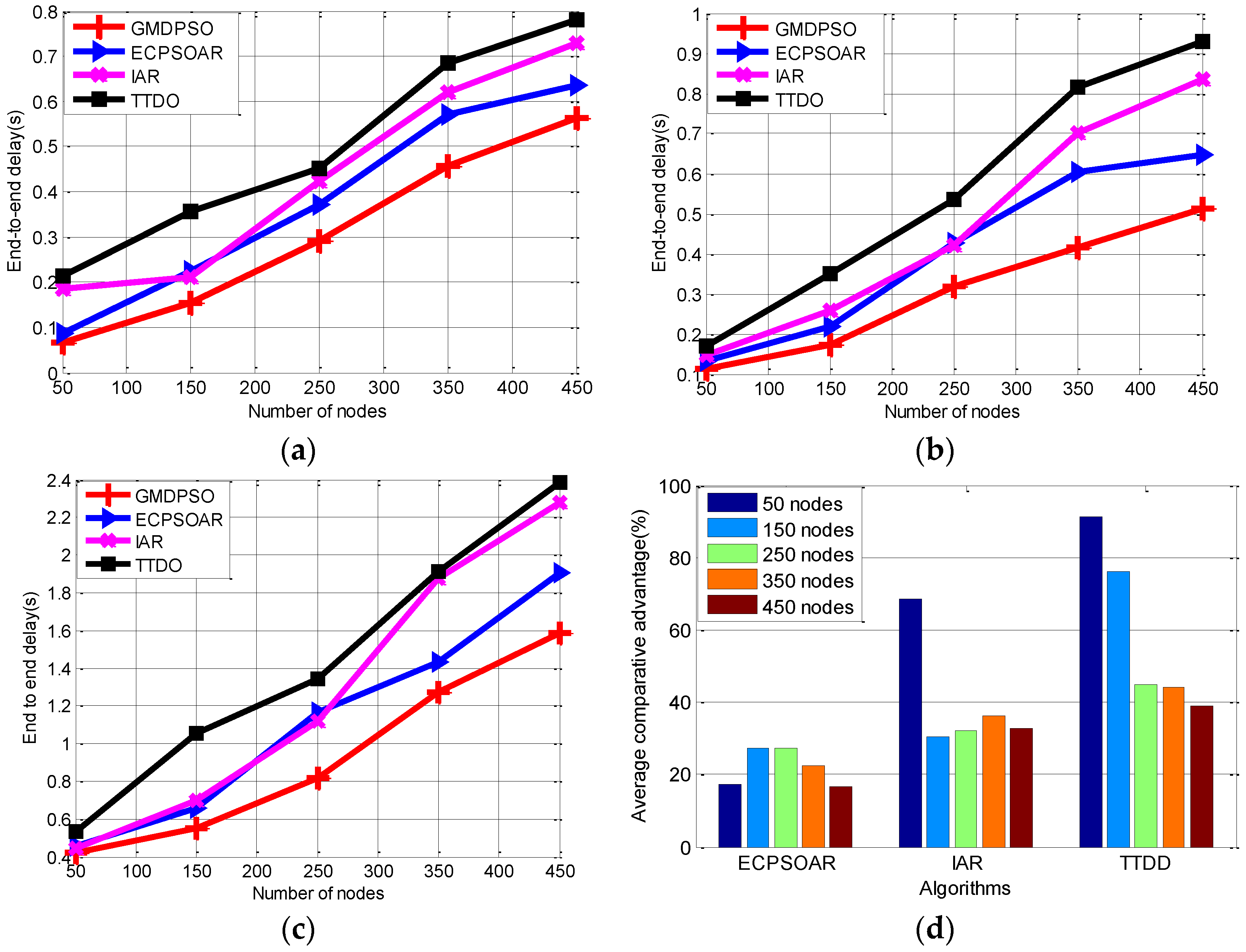
End-to-end delay is another important performance metric of MWSNs. Given a fixed channel bandwidth, less the delay, higher the throughout. Let D e l a y ( P T r e e i ) be the total communication delay of P T r e e i . Then D e l a y ( P T r e e i ) can be calculated as following:
D e l a y ( P T r e e i ) = R N j k P T r e e i d e l a y ( R N j k )
Therefore, our third objective is:
Objective   3 : Minimize  D e l a y ( P T r e e i ) = R N j k P T r e e i d e l a y ( R N j k )
Clearly, smaller D e l a y ( P T r e e i )   is better. Then our fitness is proportional to the D e l a y ( P T r e e i ) i.e.,
f i t n e s s   D e l a y ( P T r e e i )
Similar with Equation (19), D e l a y ( P T r e e i ) also can be normalized as follows:
D e l a y ( P T r e e i ) = R N j k P T r e e i d e l a y ( R N j k ) / n o d e i V d e l a y ( n o d e i )
After normalizing the above three objectives, the final fitness function for P T r e e i   is:
f i t n e s s ( P T r e e i ) = ω 1 × m i n L f P T r e e i + ω 2 × L e n ( P T r e e i ) + ω 3 × D e l a y ( P T r e e i )
where ω1, ω2 and ω3 are three control parameters, 0 < ωi ≤ 1 and ω1 + ω2 + ω3 = 1. In the paper, we give the same weight to them, that is, ω1 = ω2 = ω3 = 0.33.

5.2.2. Particles Representation

How to encode the routing tree is very critical. To make GMDPSO feasible for discrete MWSNs scenario, the position and velocity of particle in our protocol are redefined.
Definition 1 (Position). 
The position vector provides a routing tree. The position vector of ith particle is defined as Xi = { x i 1 , x i 2 , x I 3 , …, x i N }, where N   = N − 1 is dimension of Xi which means the number of candidate relay nodes excluding the agent, the d component x i d ∈ {0, N} is the sensor ID, which maps nodek (k = x i d ) as the next relay node of noded. That is to say, x i d indicates that noded forwards data to nodek.
Notably, Xi means a routing path tree that includes multi routing paths from multi source nodes to the same root node. Suppose mobile sink Sinki has NS source nodes, and then Xi includes NS routing paths. A graphical illustration of particle representation can be seen in Figure 4.
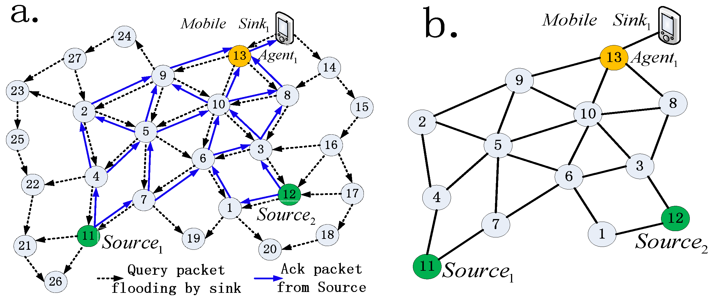
Illustration 1. 
Consider mobile sink Sinki masters a subnet of MWSN G (V, E) with 13 sensor nodes and one mobile node as shown in Figure 4a. V = {node1, node2, …, node13}. node13 is selected as agent, node11 and node12 are two source nodes, which means two routing paths will be built. The dimension of the particle position vector is N = N − 1 = 13 − 1 = 12. As shown in Figure 4b. Particle i is encoded as Xi = { x i 1 , x i 2 , x I 3 , …, x i 12 } = {6, 9, 10, 5, 9, 5, 5, 13, 13, 13, 4, 3}, in Xi, for example, x I 11 = 4 indicates that source node node11 sends data packet to node4. A routing tree is constructed by decoding the encoded particle, in which each route path from a source node to sink can be built by appending relay nodes one by one till the agent node is selected as the end.
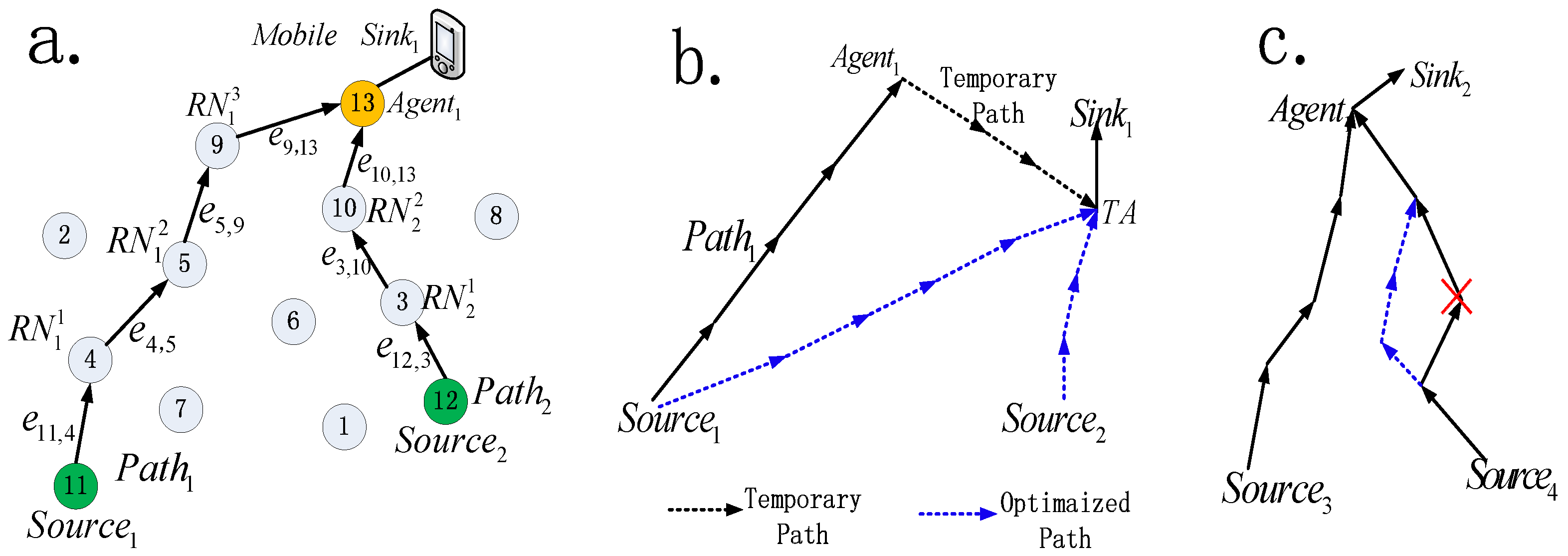
As shown in Figure 4c, the path tree can be decoded as follows: firstly, the routing path of Source1 (i.e., node11) is built as Path1: Source1→node4→node5→node9→Agent1.Then, routing path of Source2 (i.e., node12) is built as Path2:Source2→node3→node10Agent1, and at last, the whole routing tree can be constructed by combining Path1 and Path2.
It can be seen from Figure 4 that our discrete position definition is straightforward and easy to decode and will lower the computational complexity, especially in the case of large-scale MWSNs, because the dimensions of the fitness function is equal to the size of candidate relay nodes collected by sink which is smaller than the entire MWSN size.
Definition 2 (Velocity). 
Velocity is a very crucial component in PSO, by working on the position vector, it guides a particle and determines whether it can reach its destination and by how fast it could. Our discrete velocity of particle i is defined as Vi = { v i 1 , v i 2 , …,   v i N }, where v i j {0,1} is binary-coded, v i j = 1 means that the corresponding element x i j in Xi will be changed, otherwise, x i j keeps its original state. v i j and x i j have the same dimension.
In canonical PSO, velocity is used to learn knowledge from itself and swarm and finally leads the particle to a better position. In addition, a threshold Vmax is used to inhibit particles from flying out of the boundaries because there is a situation whereby when the speed of a particle is substantial. Unlike the continuous optimization, we have known that, in our discrete MWSNs scenarios, to compare two different routing paths from the same source node to the same agent, we only take care about whether their relay nodes are the same. Furthermore, we only need to compare the two relay nodes ID value in the same position of two different routing paths. There are only two results: is equal or no, therefore, the velocity can be encoded binary, and we defined 0 means two relay nodes are the same, 1 means they are different.
The first motivation of the velocity definition is to actually reflect the differences between two position vectors. The second motivation of the velocity definition is to prevent particles from flying away, because our velocity is binary-coded, we no longer need Vmax parameter.

5.2.3. Particle Swarm Initialization

A good initialization mechanism can reduce the searching space to reach global optima faster and promote diversity. Conventional random initialization method for PSO based algorithm is not applicable for our algorithm. The main reason is that random sequence of edges usually results in invalid routing tree that does not terminate on the agent node or that have loops. Therefore, we need to design a more efficient initialization method for our protocol. Based on our particle representation for discrete MWSNs, the position vectors initialization focus on how to map the next relay node, in other words, how to select the next relay node for the current one, for example, how to map another node as the next relay node for current node noded. Our main idea to solve this problem is that the next relay node for the current one is randomly selected from its neighbors. The mapping is done as follows:
Let Neig(noded) = {node1, node2, …, nodeK} = { x t j |0 ≤ j N V & 0 < A[d, j] < ∞} be the neighbors of noded, and A is the adjacent matrix for G (V, E),Then,
n o d e k = I n d e x ( N e i g ( n o d e d ) , n ) 1 n | N e i g ( n o d e d ) |
where Index (Neig(noded), n) is an indexing function that indexes nth node of Neig(noded) as the next relay node, and n is a randomly generated uniformly distributed integer number. Table 2 shows the nodes and their neighbors. Besides, Table 1 also illustrates how the next relay node is chosen.
In order to reduce the randomicity and blindness of swarm initialization, and at the same time speed up the convergence of our algorithm, the position vectors are initialized in such way:
Step 1 Agent node is forced to be mapped as the relay node of its neighbor nodes (seeing the blue number in Figure 4b. In detail, firstly, position vector of i particle is empty, that is, Xi = (0, 0, 0, 0, 0, 0, 0, 0, 0, 0, 0, 0). Then assign agent node (i.e., node13) to its neighbor nodes, as shown in Table 2, then Xi = ({0, 0, 0, 0, 0, 0, 0, 13, 13, 13, 0, 0}. Marker ‘-’ in Table 2 means that the relay node of the corresponding node is specified directly instead of choosing from its neighbors using Equation (27).
Step 2 Maps agent’s neighbors to be relay node of the agent’s neighbor’s neighbor. Notably, if some of the agent’s neighbors have the same neighbor, which cause more than one node will be mapped as the relay node of the same neighbor at the same time, and then we chose the nearest neighbor as the relay node. For example, as shown in Table 2, the neighbor of the agent (i.e., node13) is Neig (node13) = {node8, node9, node10}, then node13 is the common next relay node of Neig (node13). Next, we assign node8, node9, and node10 to their neighbors respectively. Neig(node8)∪Neig(node9)∪Neig(node10) = {node2, node3, node5, node6}, which means that node8, node9, and node10 should be assigned to node2, node3, node5 and node6 ,that is to say, the third column of Table 2 (i.e., column n) of the corresponding nodes, i.e., node8, node9, node10, node2, node3, node5 and node6 should be marked with ‘-’. It is easy to be seen form Figure 4a that Neig (node2) = node9, Neig (node6) = node10. For node5, because Neig (node9)∩Neig(node10) = {node5}, which means that node9 can be chosen as the next relay node for node5, and so do node10. We chose node9 as the relay node of node5 with assumption that node9 is the nearest neighbor of node5. For node6, we choose node10 as its next relay node in the same way. After finished Step 2, then the position vector Xi will look as following: Xi = {0, 9, 10, 0, 9, 10, 0, 13, 13, 13, 0, 0}.
Step 3 The relay nodes of remaining nodes are mapped by randomly choosing a node from their neighbor. For example, for Source1 (i.e., node11), let random n = 1, then its first neighbor is chosen as the next relay node.
Step 4 Finally, after finished the above three initiation steps, position vector Xi is initiated as Xi = {6, 9, 10, 5, 9, 10, 5, 13, 13, 13, 4, 3}.
It is worth noting that the invalid routing tree, in which contains one or more invalid routing path (that does not terminate on the agent node or that have loops), will be punished with a very high fitness.
The velocity vectors are initialized as all-zero vectors. The Pbest vectors are initialized in the same manner as the position vectors, and the vector is set as the best position vector in the original population.
Comparing to the conventional random initialization, the advantages of our initiation method are follows:
(1)
Since node can and only can select its next relay node from its neighbors based on the network topology of G(V, E), our method takes advantage of this feature to reduce the vast search space significantly.
(2)
In our method, agent node and its neighbors are mapped firstly in step1 and step3, and this reduces the likelihood of invalid routing path. In addition, it further reduces search space and drives particle to find its personal best position faster. That is, it speeds the algorithm convergence.

5.2.4. Velocity and Position Update

In canonical PSO, velocity gives a particle the moving direction and tendency. After updating its velocity, the particle builds its new position using the new velocity. However, in the proposed algorithm, the particle position and velocity vectors have been redefined in a discrete integer form, and thus, the mathematical updating rules in the canonical continuous PSO no longer fit the discrete case. In order to meet the requirements of building routing tree in discrete MWSNs, the particle’s velocity and position updating rules have been redefined as follows:
V i ( t + 1 ) = w × V i ( t ) c 1 × r 1 × ( p b e s t i X i ( t ) ) + c 2 × r 2 × ( G b e s t X i ( t ) )
  X i ( t + 1 ) = X i ( t ) V i ( t )
where w is the dimensional inertial weight vector, c1 and c2 are two N V dimensional cognitive and social components, r1 and r2 are two N V dimensional random vectors in rang [0,1]. Equation (28) is used to update the old velocity, and Equation (29) is the position updating rule. It can be observed that the new updating rules take the same form in canonical PSO but different the key operator. The following will detail our new operators in discrete PSO.
Definition 3 (Position Operator). 
⊝. Position ⊝ Position builds a velocity vector. Assume that we are given two position vector Xi = { x i 1 , x i 2 , x i 3 x i N } and Xj = { x j 1 , x j 2 , x j 3 , …, x j N }, Xi ⊝ Xj = V = {v1, v2, …, v N }, the element vd is defined as:
v d = { 0 i f x i k =   x j k 1 o t h e r w i s e
Definition 3 is inspired from the following two aspects:
First, it is well known that, in canonical PSO, a particle adjusts its velocity by learning from its old velocity (Vi(t)), personal best position (Pbesti-Xi(t)) and the swarm global best position (Gbest-Xi(t)). It can be seen that the learning process is actually a comparison between the positions, that is to say, two position vectors should generate a velocity vector. Second, two position vectors represent two different routing trees. The defined ⊝ operation actually is used to find which relay nodes are different between these two routing paths, and these differences will give a particle the fly direction.
Definition 4 (Velocity Operator). 
⊕. Velocity ⊕ Velocity is also a velocity vector. Given two velocity vectors V1 = { v 1 1 , v 1 2 , …, v 1 N } and V2 = { v 2 1 , v 2 2 , …, v 2 N }, then V3 = V1 V2 = { v 3 1 , v 3 2 , …, v 3 N }. v 3 i can be compute as follows:
v 3 k = { 1 c o n d i t i o n   1 : i f v 1 k + v 2 k 1 0    c o n d i t i o n   2 : o t h e r w i s e
Suppose V1 = PbestiXi(t) and V2 = GbestXi(t), then, condition1 means that once the kth relay node in particle i (i.e., v 1 k = 1) needs to be changed, which is decided by its own knowledge (i.e., v 1 k = 1) or by swarm knowledge (i.e., v 2 k = 1) or both of them (i.e., v 1 k = 1 & v 2 k = 1), it must be changed finally. The definition of the operator ⊕ is easy to understand and easy to perform. Moreover, it can ensure binary-coded consistency for velocity, which is easier for the position to work with.
Definition 5 (Coefficient × Velocity). 
Coefficient × Velocity is still velocity vector. Given the Coefficient ω and the velocity vector V1 = v 1 1 , v 1 2 , …, v 1 N }, then V2 = ω × V1 = { v 2 1 , v 2 2 , …, v 2 N }. Where v 2 i can be compute as follows:
v 3 i = { 1 c o n d i t i o n   1 : i f v 1 i = 1 1 c o n d i t i o n   2 : i f v 1 i = 0  &  ω 0.5 0 c o n d i t i o n   3 : i f v 1 i = 0  &  ω < 0.5
condition1 means that if a relay node needs to be changed , then change it without regard to the ω. Condition2 and condition3 are conditions for mutation operation of particle, which means that although a relay node does not need to be changed(i.e., v 1 i = 0), it still maybe be changed in a mutation probability (i.e., 0.5). Mutation operation of particle can promote the diversity of particles and avoid falling into the local optimum.
Definition 6 (Position Updating Operator)
⊗. ⊗ is very important component in our update rules, which is used by particle to update its position with its new velocity. Position ⊗ Velocity generates a new position. A good design for operator ⊗ should drive a particle to a better position. Given an old position Xt = { x t 1 , x t 2 , …, x 2 N } and a new velocity Vt+1 = { v t + 1 1 , v t + 1 2 , …, v t + 1 N }, then the new position Xt+1 = Xt ⊗ Vt+1 = { x t + 1 1 , x t + 1 2 , …, v t + 2 N }, the element x t + 1 i of Xt+1 can be computed as follows:
x t + 1 i = { b e s t R N i i f   v t + 1 i = 1  &  x t i P a t h j t + 1   x t i o t h e r w i s e
where x t j P a t h j t + 1 means that the old node x t j is selected as a relay node in the P a t h j t + 1 in Xt+1, in other words, if x t j is not a relay node, it need not to be changed. Notably, Xi means a routing path tree that contains NS routing path branches, and Pathj is only one routing path branch of the routing path tree. Therefore, only these old nodes will be changed that satisfies the following conditions simultaneously: they are chosen as the relay nodes and their corresponding velocities are set to 1, i.e. v t + 1 i = 1  &  x t i P a t h j t + 1 . bestRNi is the node ID which can be calculated by:
b e s t R N i   = arg min k φ ( i , k | k N e i g ( i ) )
argmink f(k) returns the value of k that minimizes f(k). φ is calculated using the following equation:
φ ( i , j | k N e i g ( i ) )   = f i t ( P a t h j ( i k ) )
where i→k means that nodek is chosen as the next relay node of nodei. fit(x) is the fitness function (i.e., Equation (26)), and fit(Pathj(i→k)) means that we only calculate the fitness value of the two adjacent relay nodes in Pathj. Similar to greedy forwarding mechanism, Equation (35) means we choose the best next relay node for the current node from all its neighbors. However, unlike greedy mechanism that only chooses the nearest neighbor as the best next relay node, our approach chooses the neighbor node, which achieves the best balance of lifetime, distance and delay as the best next relay node by using our fitness function. Therefore, with the beginning from Sourcej. Pathj can be built by selecting the best relay node one after one until the agent node is chosen, and Pathj that is built in this way is the optimal routing path. For example, let first bestRN1 be R N j 1 , then P a t h j 1 = ( S o u r c e j R N j 1 ) is the current optimal routing path. Let P a t h j 2 be the bestRN2 of R N j 1 , P a t h j 2 = ( R N j 1 R N j 2 ) is the current optimal routing path. Then,
P a t h j 1 = ( S o u r c e j R N j 1 ) P a t h j 2 = ( R N j 1 R N j 2 ) } P a t h j = ( S o u r c e j R N j 1 R N j 2 )
where Pathj is also the optimal routing. Using the same way, the other routing branches of Xt can be built. Next, the fitness of the Xt can be calculated using Equation (26).
This search mechanism of bestRNi (i.e., Equation (34)) actually act as our particle searching strategy in GMDPSO, in which a particle update its position by selecting the next relay node that can generate the largest decrement of the fitness value, so it can be regard as a greedy local search strategy.
Our motivation of searching bestRNi in this way is based on the divide-conquer strategy, in order to build an optimal routing tree of Xt, we firstly build each optimal routing path branch of Xi respectively. When all routing path branches are built completely, then, the whole routing path tree is finished. Similarly, in order to build the optimal routing path branch Pathj, we choose the best next relay node for the previous relay node one after one, until the whole Pathj is completed.
However, Equation (34) is only used to build the single optimal routing path branch, rather than build the routing path tree (i.e., Xi). Because when we choose the best relay node for the current node of Pathj, we do not consider the effect of the other routing path branch. Therefore, this method may neglect such a case, each routing branch is optimal, but the whole routing tree are weak due to the intersection relay nodes of multi routing paths. In other words, optimal routing path branches do not mean the optimal routing tree. As shown in Figure 5, many source nodes send their data packets to same next relay node, and these relay nodes will consume more energy to forward more packets. For example, node6 need forward data packets of Source1, Source2 and Source3 to node10, while, node10 needs forward data packets of Source1, Source2, Source3, Source4 and Source5 to Agent1. The worst result is that these sharing relay nodes will die quickly because they deplete their energy of forwarding too many packets. This will lead to the expensive routing recover.
Therefore, after all of individual optimal routing path branches are built, the corresponding routing tree Xi should be evaluated using fitness function.
From the above description of our new GMDPSO algorithm, the proposed algorithm has the following features: (1) with a concise framework; (2) the newly defined particle position and velocity are direct and easy to decode; and (3) redefined updating rules based on the new operators are easy to realize and will significantly reduce the computational complexity, especially for large-scale WSNs.

6. The Redesigned GMDPSO Seems to be Very Suitable for Solving Routing Problem in MWSNs6. Simulations and Results

In this section, we test our protocol against several well-known protocols: ECPSOAR, IAR, and TTDD, which all can deal with routing problem of multi mobile sinks. The performance is compared in terms of the following metrics: average packet delivery ratio (PDR, measured as the average number of successfully delivered packets versus required packets per round), average end-to-end delay (EED) [29], and average energy consumption ratio (ECR, measured as the average energy consumption from source to sink versus the initial energy per round). All simulations are performed using MATLAB R2012b on Windows 7 with Intel core i5-2520M Dual-Core CPU (2.50 GHz) and 8 G RAM. For ease of description for the comparison results of the above metrics, we define another notation, which is called metric comparative advantage for our new protocol as defined below:
M e t r i c   c o m p a r a t i v e    a d v a n t a g e =            ( M e t r i c   o f   G M D P S O     M e t r i c   o f   o t h e r   p r o t o c o l ) M e t r i c   o f   o t h e r   p r o t o c o l × 100
For example, PDR comparative advantage to ECSPOAR can be calculated as follow:
P D R   c o m p a r a t i v e    a d v a n t a g e   t o   E C P S O A R =             ( P D R   o f   G M D P S O   -   P D R   o f   E C P S O A R ) P D R   o f   E C P S O A R × 100

6.1. Simulation Setting

Simulations are performed on the MWSN, which consists of diverse number of homogenous sensor nodes ranging from 50 to 450. Each sensor node is assumed to have initial energy of 120 J and the mobile sink is assumed to have sufficient energy and cannot be fault.
To build a level playing field, the characteristics of the networks and communication models are configured as illustrated in [10] and as shown in Table 3. The extra PSO parameters used for ECPSOA are fixed to: particle updating energy consumption EPU = 80 pJ the endocrine selection energy consumption EES = 50 pJ at per iteration, function dimension D = 30, division factory k = 6, and maximum iteration PGen = 800 .The extra PSO parameters used for GMDPSO are fixed to: ω = 0.7968, c1 = c2 = 1.4926 In addition, the population size of ECPSOA and DPSORR is set to be 60; both of the two algorithms are run for maximum of 800.
For the weight sum approach, in our proposed algorithms, we give equal weight to each sub-objective. That to say, we set w1 = w2 = w3 = 0.33.

6.2. Results and Analysis

6.2.1. Performance of GMDPSO

First, we compare the performance of the proposed GMDPSO with ECPSOA, standard PSO [30] and the CPSOA [31]. In order to ensure a fair comparison, we configure these tree algorithms based on the same fitness function in Equation (26) with 450 sensor nodes, all simulation parameters are set to the same value, and the iterated generation for three protocols is fixed to 300.
The test result is shown in Figure 6. It can be seen that: GMDPSO outperforms the other PSOAs in term of convergence rate and the minimum fitness value. This is mainly due to the greedy search strategy based on the MWSNs topology, which avoid the blind search of the particle; another reason is that the memory mechanism reduces the repeated and invalid searching. It also can be seen that GMDPSO has the best initial fitness value, which is achieved by our special particle initial mechanism.

6.2.2. Packet Delivery Ratio

A routing protocol’s reliability depends on PDR to the sink. Here, we run these protocols for comparing average PDR. Figure 7 and Table 4 show the comparison results when the speed of sinks is 5 m/s. Figure 7 shows that our protocol is more reliable and robust. In detail, firstly, average PDR of all protocols are decreasing as the number of nodes increases; however, our protocol still outperforms the others and the advantage (i.e., Equation (17)) is becoming more and more obvious as the number of sensor nodes increase in Figure 7d. Secondly, PDR reduces with the increase of the node failure probability (Figure 7a–c). Still, our protocol can deliver more packets than the other protocols with the same network size. Thirdly, with each same P f a u l t ,t, our protocol always keeps the maximum average PDR (Figure 7a–c), which means that our protocol can find a better solution than others respect to different sensor nodes. Meanwhile, Table 4 illustrated that, with each same sensor node, our protocol keeps the maximum average PDR, which means that our protocol can find a better solution than others respect to different P f a u l t . That is to say, no matter with different sensor nodes or different node failure probability, our protocol can find the best path tree among the 4 protocols. Therefore, based on the above two results, we conclude that our protocol is more robust in PDR.
Our protocol improved the average PDR noticeably due to the following three reasons: The first reason is, the temporary path (TP) is designed to continue the old data packets transmission when sink moves away the old agent, which can avoid the packets loss before the new optimal routing path coming into services. The second reason is: our protocol can quickly locate the failure node and quickly build an alternative optimal path to recover the broken path link by its fast convergence feature and without any flooding when relay nodes fail, which also can reduce the data packets loss. The third reason is: the proposed GMDPSO can build better alternative routing path than others due to its ability of achieving global optimum, such as shorter total transmission distance and small communication delays, which can enhance the communication reliability and PDR. Moreover, our fitness function minimizes the energy consumption of the relay nodes to reduce the premature death probability of the relay node, which also can reduce the data packets loss due to the broken routing path.

6.2.3. End-to-End Delay

Next, we compare the average EED of the proposed protocol on the same experiment environment as Section 6.2.1. Figure 8 and Table 5 show the comparison result. It can be observed from Figure 8 that the proposed protocol has smaller end-to-end delay than the existing protocols.
More specifically, firstly, with the increase of the number of nodes, EED of all these protocols is increased. Again, our protocol performs best. This is because our protocol adopts the GMDPSO algorithm, whose better performance in reaching the global optimum allows it to build the optimal routing tree with shorter transmission distance. Furthermore, its faster convergence feature make it can build the optimal routing tree more quickly. Moreover, by using our neighbor table, the routing information is stored in each node to improve the speed of route establishment. All these advantages of GMDPSO can help to decrease the end-to-end delay. It is worthy to note that, as illustrated in Figure 8d, the average EED comparative advantage (i.e., Equation (17)) decreases as the number of sensor nodes increases, this is because our greedy search rule spends more time to select the best relay nodes from larger scale nodes to build the optimal routing tree. Nevertheless, the fast response of routing recovery and less communication control overhead by our unicast flooding mechanism also make our protocol end-to-end delay lower than the other protocols. Secondly, the end-to-end delay increases with the increase of the node failure probability by comparing Figure 8a–c, as the less stable topology causes more route recovery operation, which consumes more time for the protocols to maintain the network and prolong the delay. However, our protocol can still achieve the optimal delay; this is because we have designed the quick routing recovery mechanism for failure relay nodes. Thirdly, similar to average PDR, it can be observed from Figure 8a–c and Table 5 that our protocol achieves best average EED with respect to different sensor nodes and different P f a u l t , which means that our protocol can find a better solution than others. That to say, our protocol keeps better robustness of EED, this is because that the GMDPSO adopted in our protocol can also build the global optimum routing tree in different network size, however, others maybe build different suboptimal routing solutions for different network sizes, which increase the volatility of delay. Moreover, once the existing routing path is broken due to failure nodes, an alternative optimal path can be quickly established for the source node in our protocol. In addition, the other failure nodes (i.e., not the relay nodes) never be selected as the relay nodes due to our fitness function.

6.2.4. Energy Consumption

Although mobile sink protocol can alleviate hotspots implicitly by changing the possible high energy consumption zones around the sinks as the sinks move. However, these operations may cause the overall energy consumption in the network to increase. Now, we compare the average ECR of these protocols, which is used to measure the influence of node failure probability and mobile sink speed to the network. Simulations are performed on different network sizes with different sink speeds (speed of 5 m/s, 10 m/s and 20 m/s). Here, the node failure probability is set to 0.1. Figure 9 and Table 6 illustrate that the energy consumption of our protocol is the smallest among these protocols, and the comparative advantage (i.e., Equation (17)) becomes larger as the number of sensor nodes increases in Figure 9d. It worth to note that the average ECR of all these protocols increases as the mobile sinks move faster, because the change of the frequent topology results in frequent routing recovery which introduces heavier communication and energy overhead due to flooding operation. In this situation, our protocol can still consume less energy than the other protocols with the same network size. Besides, similar to average PDR, we can also conclude that our protocol achieves better robustness of EED than others from Figure 9a–c and Table 6.
Our protocol outperforms others in term of ECR. The main reasons are as follows: the improved greedy forwarding mechanism is used ensure each routing branch has the mining energy consumption by selecting the relay node with optimized QoS parameters (energy, delay, energy consumption and so on). In addition, the unicast local flooding mechanism reduces the communication overhead in the network, which can minimize and indirectly reduce energy consumption.
In summary, the overall performance of our protocol outperforms LEACH, SEP, ERP and TPSO-CR in terms of the PDR, EED and EDR, while maintaining the best robust.

7. Conclusions

In this paper, the routing of MWSNs is formulated as an optimization problem and we employ PSO to design an efficient routing protocol to achieve higher energy efficiency and lower communication delay. However, conventional PSO was originally designed for continuous optimization problems, which limits its application in discrete optimization domains. In addition, conventional PSO suffers from the curse of dimensionality, i.e., its performance deteriorates quickly as the dimensionality of the search space increases exponentially. To address these problems, we design a novel GMDPSO to build the optimal route tree. In GMDPSO, we first deduced a new more suitable fitness function, then redefined the particle position and velocity in a discrete form and subsequently redesigned the particle update rules based on the network topology; consequently a discrete PSO framework was established. When applying the proposed discrete PSO framework to solve the mobile sink route problem, to alleviate prematurity, a greedy local search based method was specially designed for the particle position update rule by improving the greedy forwarding mechanism. Simulations demonstrated that the proposed protocol is effective and promising.

Acknowledgments

The authors would like to thank the anonymous reviewers and guest editor for their valuable reviews that are very useful for the improvement of quality of this paper. This work was partially supported by the Second Batch of Strategic Emerging Industrial Core Technology Research Project in Guangdong Province under Grant No. 2012A010701005; the Key Lab of cloud computing and big data in Guangzhou under Grant No. SITGZ [2013]268-6; Engineering and Technology Research Center of Guangdong Province for Big Data Intelligent Processing under Grant No. GDDST[2013]1513-1-11; Key Project of the Combination of “Production, Education and Research” supported by Guangdong province and Ministry of Education, under Grant No. 2012B091000109 and Science and Technology Program in Guangzhou, China (International Science and Technology Cooperation Program) under Grant No. 2012J5100018; The Natural Science Foudation of Guangdong Province, under Grant No.2014A030313585; Guang Dong Provincial Natural fund project, under Grant No. 2016A030310300.

Author Contributions

Fagui Liu and Jin Yang defined problem and developed the ideal. Jin Yang, Jianneng Cao and Liangming Wang carried out the experiments and data analysis and wrote the relevant sections.

Conflicts of Interest

The authors declare no conflict of interest.

References

  1. Rault, T.; Bouabdallah, A.; Challal, Y. Energy efficiency in wireless sensor networks: A top-down survey. Comput. Netw. 2014, 67, 104–122. [Google Scholar] [CrossRef]
  2. Jaichandran, R.; Irudhayaraj, A.A.; Raja, J.E. Effective Strategies and Optimal Solutions for Hot Spot Problem in Wireless Sensor Networks (WSN). In Proceedings of the 2010 10th International Conference on Information Sciences Signal Processing and their Applications (ISSPA), Kuala Lumpur, Malaysia, 10–13 May 2010; pp. 389–392.
  3. Francesco, M.D.; Das, S.K.; Anastasi, G. Data Collection in Wireless Sensor Networks with Mobile Elements: A Survey. ACM Trans. Sens. Netw. 2011, 8. [Google Scholar] [CrossRef]
  4. Liang, W.; Luo, J.; Xu, X. Prolonging Network Lifetime via a Controlled Mobile Sink in Wireless Sensor Networks. In Proceedings of the 2010 IEEE Global Telecommunications Conference (GLOBECOM 2010), Miami, FL, USA, 6–10 December 2010. [CrossRef]
  5. Nazir, B.; Hasbullah, H. Mobile Sink based Routing Protocol (MSRP) for Prolonging Network Lifetime in Clustered Wireless Sensor Network. In Proceedings of the 2010 International Conference on Computer Applications and Industrial Electronics (ICCAIE), Kuala Lumpur, Malaysia, 5–8 December 2010; pp. 624–629.
  6. Oh, S.; Yim, Y.; Lee, J.; Park, H.; Kim, S.H. Non-Geographical Shortest Path Data Dissemination for Mobile Sinks in Wireless Sensor Networks. In Proceedings of the 2011 IEEE Vehicular Technology Conference (VTC Fall), San Francisco, CA, USA, 5–8 September 2011. [CrossRef]
  7. Liu, X.; Zhao, H.; Yang, X.; Li, X. SinkTrail: A Proactive Data Reporting Protocol for Wireless Sensor Networks. IEEE Trans. Comput. 2013, 62, 151–162. [Google Scholar] [CrossRef]
  8. Shi, G.; Zheng, J.; Yang, J.; Zhao, Z. Double-Blind Data Discovery Using Double Cross for Large-Scale Wireless Sensor Networks With Mobile Sinks. IEEE Trans. Veh. Technol. 2012, 61, 2294–2304. [Google Scholar]
  9. Tunca, C.; Isik, S.; Donmez, M.Y.; Ersoy, C. Distributed Mobile Sink Routing for Wireless Sensor Networks: A Survey. IEEE Commun. Surv. Tutor. 2014, 16, 877–897. [Google Scholar] [CrossRef]
  10. Hu, Y.F.; Ding, Y.S.; Ren, L.H.; Hao, K.R.; Han, H. An endocrine cooperative particle swarm optimization algorithm for routing recovery problem of wireless sensor networks with multiple mobile sinks. Inf. Sci. 2015, 300, 100–113. [Google Scholar] [CrossRef]
  11. Hu, Y.F.; Wu, X.M.; Wang, F.Q.; Han, H. A particle swarm algorithm based routing recovery method for mobile sink wireless sensor networks. In Proceedings of the 26th Chinese Control and Decision Conference (2014 CCDC), Changsha, China, 31 May–2 June 2014; pp. 887–892.
  12. Hu, Y.F.; Wu, X.M.; Wang, F.Q.; Liu, X.Z.; Han, H. A novel routing recovery strategy based on particle swarm algorithm for wireless sensor networks with multiple mobile sinks. In Proceedings of the 2014 13th International Conference on Control Automation Robotics & Vision (ICARCV), Singapore, 10–12 December 2014; pp. 681–686.
  13. Chengetanai, G.; Reilly, G.B.O. Review of swarm intelligence routing algorithms in wireless mobile ad hoc networks. In Proceedings of the 2015 IEEE 9th International Conference on Intelligent Systems and Control (ISCO), Coimbatore, India, 9–10 January 2015. [CrossRef]
  14. Tang, D.; Cai, Y.; Zhao, J.; Xue, Y. A quantum-behaved particle swarm optimization with memetic algorithm and memory for continuous non-linear large scale problems. Inf. Sci. 2014, 289, 162–189. [Google Scholar] [CrossRef]
  15. Luo, H.; Ye, F.; Cheng, J.; Lu, S.; Zhang, L. TTDD: Two-Tier Data Dissemination in Large-Scale Wireless Sensor Networks. Wirel. Netw. 2005, 11, 161–175. [Google Scholar] [CrossRef]
  16. Kweon, K.; Ghim, H.; Hong, J.; Yoon, H. Grid-Based Energy-Efficient Routing from Multiple Sources to Multiple Mobile Sinks in Wireless Sensor Networks. In Proceedings of the ISWPC 2009 4th International Symposium on Wireless Pervasive Computing, Melbourne, Australia, 11–13 February 2009. [CrossRef]
  17. Minhan, S.; Chunum, K.; Choo, H. Hexagonal path data dissemination for energy efficiency in wireless sensor networks. In Proceedings of the 2009 International Conference on Information Networking, Chiang Mai, Thailand, 21–24 January 2009; pp. 1–5.
  18. Kim, H.S.; Abdelzaher, T.F.; Kwon, W.H. Minimum-energy asynchronous dissemination to mobile sinks in wireless sensor networks. In Proceedings of the 1st International Conference on Embedded Networked Sensor Systems, Los Angeles, CA, USA, 5–7 November 2003; pp. 193–204.
  19. Tunca, C.; Isik, S.; Donmez, M.Y.; Ersoy, C. Ring Routing: An Energy-Efficient Routing Protocol for Wireless Sensor Networks with a Mobile Sink. IEEE Trans. Mob. Comput. 2015, 14, 1947–1960. [Google Scholar] [CrossRef]
  20. Kim, J.W.; In, J.S.; Hur, K.; Kim, J.W.; Eom, D.S. An intelligent agent-based routing structure for mobile sinks in WSNs. IEEE Trans. Consum. Electron. 2010, 56, 2310–2316. [Google Scholar] [CrossRef]
  21. Lee, J.H.; Kim, J.M.; Jang, B.T.; Lee, E.-S. Data Dissemination Protocol Based on Home Agent and Access Node for Mobile Sink in Mobile Wireless Sensor Networks. In Proceedings of the 5th International Conference on Convergence and Hybrid Information Technology (ICHIT 2011), Daejeon, Korea, 22–24 September 2011; Lee, G., Howard, D., Ślęzak, D., Eds.; Springer Berlin Heidelberg: Berlin, Germany, 2011; pp. 306–314. [Google Scholar]
  22. Jiang, Y.; Shi, W.; Wang, X.; Li, H. A distributed routing for wireless sensor networks with mobile sink based on the greedy embedding. Ad Hoc Netw. 2014, 20, 150–162. [Google Scholar] [CrossRef]
  23. Yang, H.; Ye, F.; Sikdar, B. SIMPLE: Using Swarm Intelligence Methodology to Design Data Acquisition Protocol in Sensor Networks with Mobile Sinks. In Proceedings of the 25th IEEE International Conference on Computer Communications, Barcelona, Spain, 23–29 April 2006. [CrossRef]
  24. Yang, W.; Xing, P.; Liu, Y. A positioning method of WSN based on self-adapted RSSI distance model. Chin. J. Sens. Actuators 2015, 28, 137–141. [Google Scholar]
  25. Chen, Y.; Wang, Z.; Ren, T.; Lv, H. Lifetime Optimization Algorithm with Mobile Sink Nodes for Wireless Sensor Networks Based on Location Information. Int. J. Distrib. Sens. Netw. 2015. [Google Scholar] [CrossRef]
  26. Yang, G.; Xu, H.; He, X.; Wang, G.; Xiong, N.; Wu, C. Tracking Mobile Sinks via Analysis of Movement Angle Changes in WSNs. Sensors 2016, 16. [Google Scholar] [CrossRef] [PubMed]
  27. Ahmad, A.; Rathore, M.M.; Paul, A.; Chen, B.W. Data Transmission Scheme Using Mobile Sink in Static Wireless Sensor Network. J. Sens. 2015, 2015. [Google Scholar] [CrossRef]
  28. Konak, A.; Coit, D.W.; Smith, A.E. Multi-objective optimization using genetic algorithms: A tutorial. Reliab. Eng. Syst. Saf. 2006, 91, 992–1007. [Google Scholar] [CrossRef]
  29. Maia, G.; Guidoni, D.L.; Viana, A.C.; Aquino, A.L.L.; Mini, R.A.F.; Loureiro, A.A.F. A distributed data storage protocol for heterogeneous wireless sensor networks with mobile sinks. Ad Hoc Netw. 2013, 11, 1588–1602. [Google Scholar] [CrossRef]
  30. Hu, M.; Wu, T.; Weir, J.D. An Adaptive Particle Swarm Optimization With Multiple Adaptive Methods. IEEE Trans. Evol. Comput. 2013, 17, 705–720. [Google Scholar] [CrossRef]
  31. Lin, C.-J.; Chen, C.-H.; Lin, C.-T. A hybrid of cooperative particle swarm optimization and cultural algorithm for neural fuzzy networks and its prediction applications. IEEE Trans. Syst. Man Cybern. C Appl. Rev. 2009, 39, 55–68. [Google Scholar]
Figure 1. Illustration of (a) sink queries MWSN; (b) graphic description of MWSN.
Sensors 16 01081 g001
Figure 2. (a) Illustration for routing tree; (b) Routing recover for mobile moves away; (c) Routing recover for relay node failed.
Sensors 16 01081 g002
Figure 3. Flowchart of new routing protocol.
Sensors 16 01081 g003
Figure 4. (a) Network topology; (b) Position vector encoded for (a); (c) Routing tree decoded from (b).
Sensors 16 01081 g004
Figure 5. Multi routing paths share some relay nodes.
Sensors 16 01081 g005
Figure 6. Compare of convergence.
Sensors 16 01081 g006
Figure 7. Average packet delivery ratio with respect to different node failure probabilities. (a) When the node failure probability is 0.01; (b) When the node failure probability is 0.02; (c) When the node failure probability is 0.04; (d) Average PDR comparative advantage.
Sensors 16 01081 g007
Figure 8. Average end-to-end delay with respect to different node failure probabilities. (a) When the node failure probability is 0.01; (b) When the node failure probability is 0.02; (c) When the node failure probability is 0.04; (d) Average EED comparative advantage.
Sensors 16 01081 g008
Figure 9. Average energy consumption ratio (ECR) with respect to different speeds of mobile sinks. (a) When the moving speed of sinks is 5 m/s; (b) When the moving speed of sinks is 10 m/s; (c) When the moving speed of sinks is 20 m/s; (d) Average ECR comparative advantage.
Sensors 16 01081 g009
Table 1. Neighbor table.
self_IDneighbor_IDDisisRelay
73201
79150
Table 2. Next relay node selection for position initiation.
nodedNeig(noded)nNextRelay(noded)
node1{node3, node6, node12}2node6
node2{node4, node5, node9}-node9
node3{node6, node8, node10, node12}-node10
node4{node2, node5, node7, node11}2node5
node5{node2, node4, node6, node7, node9, node10}-node9
node6{node1, node3, node5, node7, node10}-node10
node7{node4, node5, node6, node11}2node5
node8{node3, node10, node13}-node13
node9{node2, node5, node10, node13}-node13
node10{node3, node5, node6, node8, node9, node13}-node13
node11{node4, node7}1node4
node12{node1, node3}2node3
node13{node8, node9, node10, sink}sink
Blue color means the corresponding node are mapped in step1. Green color means the corresponding node are mapped in step 2.Black color means the corresponding node are mapped in step 3.
Table 3. Simulation parameters.
ParameterValueParameterValue
Area5000 × 5000 m2Packet size1 KB
Sensor nodes50, 150, 250, 350, 450Deliver packets rate20 per round
Mobile sinks5Simulation iterations number200
Initial energy of nodes120 Jα160 nj/bit
communication rang600 mβ145 nj/bit
sensing rang R300 mβ210 nj/bit
Speed of mobile vsink5 m/s, 10 m/s, 20 m/sγ1135 nj/bit
Pfault0.1, 0.2, 0.4Channel attenuation n2
Table 4. Average packet delivery ratio (PDR) with respect to different P f a u l t .
Algorithms 150 Sensor Nodes 350 Sensor Nodes 450 Sensor Nodes
P f a u l t .01 P f a u l t .02 P f a u l t .04 P f a u l t .01 P f a u l t .02 P f a u l t .04 P f a u l t .01 P f a u l t .02 P f a u l t .04
GMDPSO0.9240.8520.8210.8430.7810.7210.7940.7280.694
ECPSOAR0.8960.8140.7710.8030.7210.6340.7360.6430.571
IAR0.8290.7730.6790.7370.6260.5950.6330.5710.456
TTDD0.7550.68900.6980.6700.6430.5510.6200.5670.486
Table 5. Average end-to-end delay (EED) with respect to different P f a u l t .
Algorithms 150 Sensor Nodes 350 Sensor Nodes 450 Sensor Nodes
P f a u l t .01 P f a u l t .02 P f a u l t .04 P f a u l t .01 P f a u l t .02 P f a u l t .04 P f a u l t .01 P f a u l t .02 P f a u l t .04
GMDPSO0.1550.1730.5510.4570.4171.2730.5630.5131.585
ECPSOAR0.2230.2200.6590.5710.6051.4310.6350.6461.908
IAR0.2120.2600.7000.6200.7021.8780.7290.8352.278
TTDD0.3570.3491.0560.6840.8151.9110.7800.9292.383
Table 6. Average ECR with respect to different V S i n k .
Algorithms 150 Sensor Nodes 350 Sensor Nodes 450 Sensor Nodes
V S i n k 5 V S i n k 10 V S i n k 20 V S i n k 5 V S i n k 10 V S i n k 20 V S i n k 5 V S i n k 10 V S i n k 20
GMDPSO0.2640.3020.3520.3820.4820.5490.4160.5390.618
ECPSO0.3210.3410.3950.4870.6050.6340.5120.6460.749
IAR0.3360.4450.4860.6070.7020.7370.6430.8350.880
TTDS0.4050.5120.5600.6180.8150.8690.7280.9290.941

