An automatic detection and localization of underwater objects is of great importance in Autonomous Underwater Vehicle (AUV) navigation and mapping applications. Object detection aims at separating a foreground object from the background and generating a binary image for every frame, which is of critical importance for the sonar image processing since the result will directly affect the accuracy of the following feature extraction and object localization [
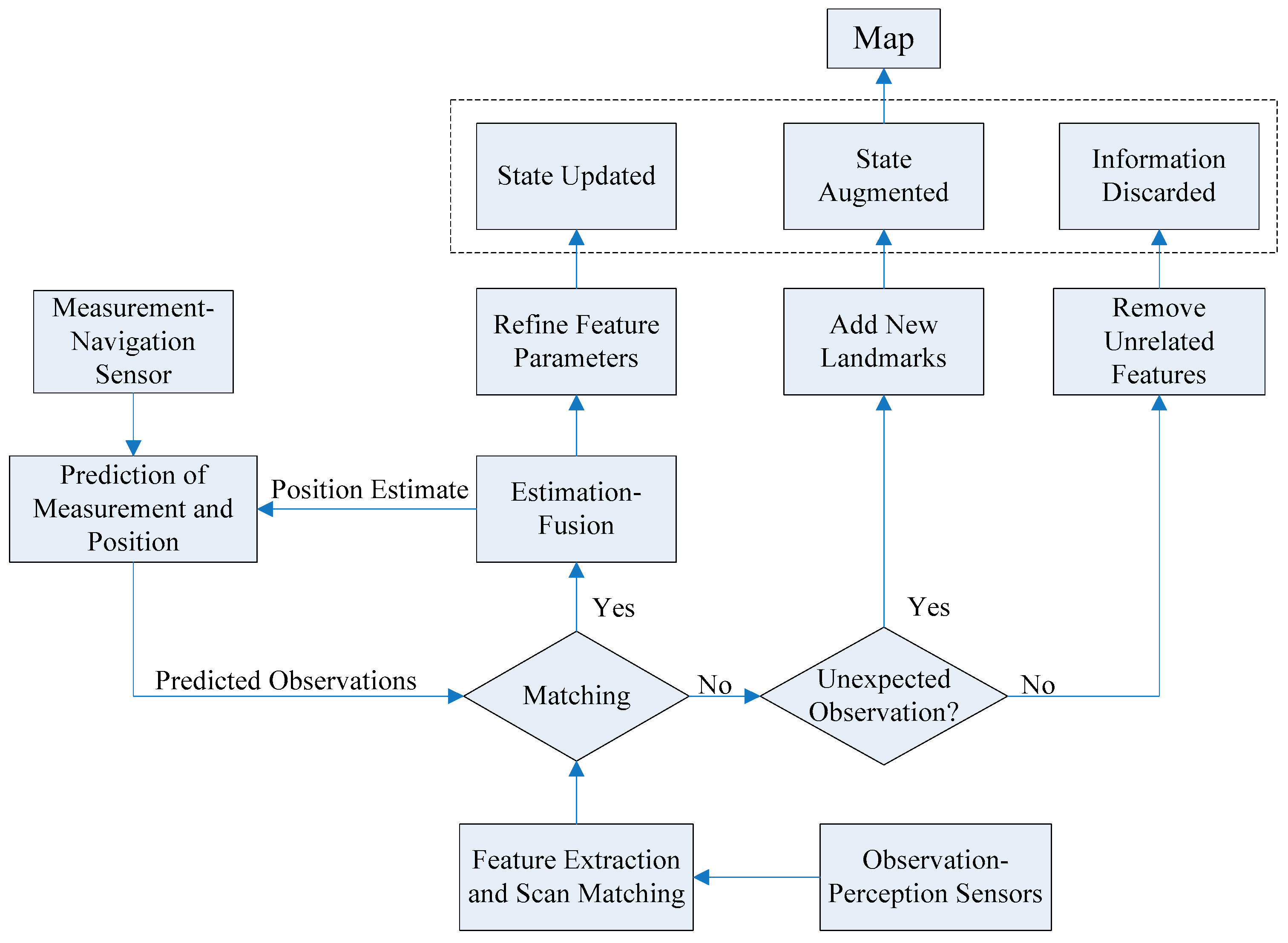
36]. Feature extraction is an important aspect of SLAM, in which a mobile robot with a known kinematic model, starting at an unknown location, moving through the exploring environment where contains multiple features to incrementally generate a consistent map. Geometric features, such as points, lines, circles and corners are determined as a part of the SLAM process, since these features can be used as landmarks. Generally, SLAM consists of the following parts including motion sensing, environment sensing, robot pose estimation, feature extraction and data association. The main focus of this paper is on first extracting features from underwater sonar images of different types, and then using them as landmarks for an AEKF-based underwater SLAM.
In recent years, the resolution of sonar imagery has improved significantly, such that it can be used in a much better way for further processing and analyzed with advanced digital image processing techniques. Noise filtering, radiometric corrections, contrast enhancement, deblurring through constrained iterative deconvolution, and feature extraction are usually employed to correct or to alleviate flaws in the recorded data [
37]. The first step of underwater object detection is to segment the foreground features from the background. Segmentation is the process of assigning a label to every pixel in the image such that pixels with the same label share homogeneous characteristics, like color, intensity, or texture, and thereby different entities visible in the sonar imagery could be separated. A sonar image is made up of a matrix of pixels having a gray level typically on a scale from 0 to 255. The gray levels of pixels associated with foreground objects are essentially different from those belonging to the background. Normally, in typical sonar imagery, the object is composed of two parts: the highlighted areas (echo) and the shadow regions. The echo information is caused by the reflection of the emitted acoustic wave on the object while the shadow zones correspond to the areas lack of acoustic reverberation behind the object. Based on this characteristic, the threshold segmentation methods (TSM) can be used to detect the foreground object in the sonar image. In general, the Otsu method is one of the most successful adaptive methods for image thresholding [
38].
3.1. Side-Scan Sonar Images
Under optimal conditions, side-scan sonars (SSS) can generate an almost photorealistic, two-dimensional picture of the seabed. Once several swatches are joined via mosaicing, geological and sedimentological features could be easily recognized and their interpretation would provide a valuable qualitative insight into the topography of the seabed [
39]. Due to the low grazing angle of the SSS beam over the seabed, SSS provide far higher quality images than forward-looking sonars (FLS), such that the feature extraction and the data association processes will behave better. The accuracy of SLAM using SSS is more dependent on the distribution of landmarks. In general, the SSS and the multibeam FLS provide large scale maps of the seafloor that are typically processed for detecting obstacles and extracting features of interest on the areas of the seafloor [
18].
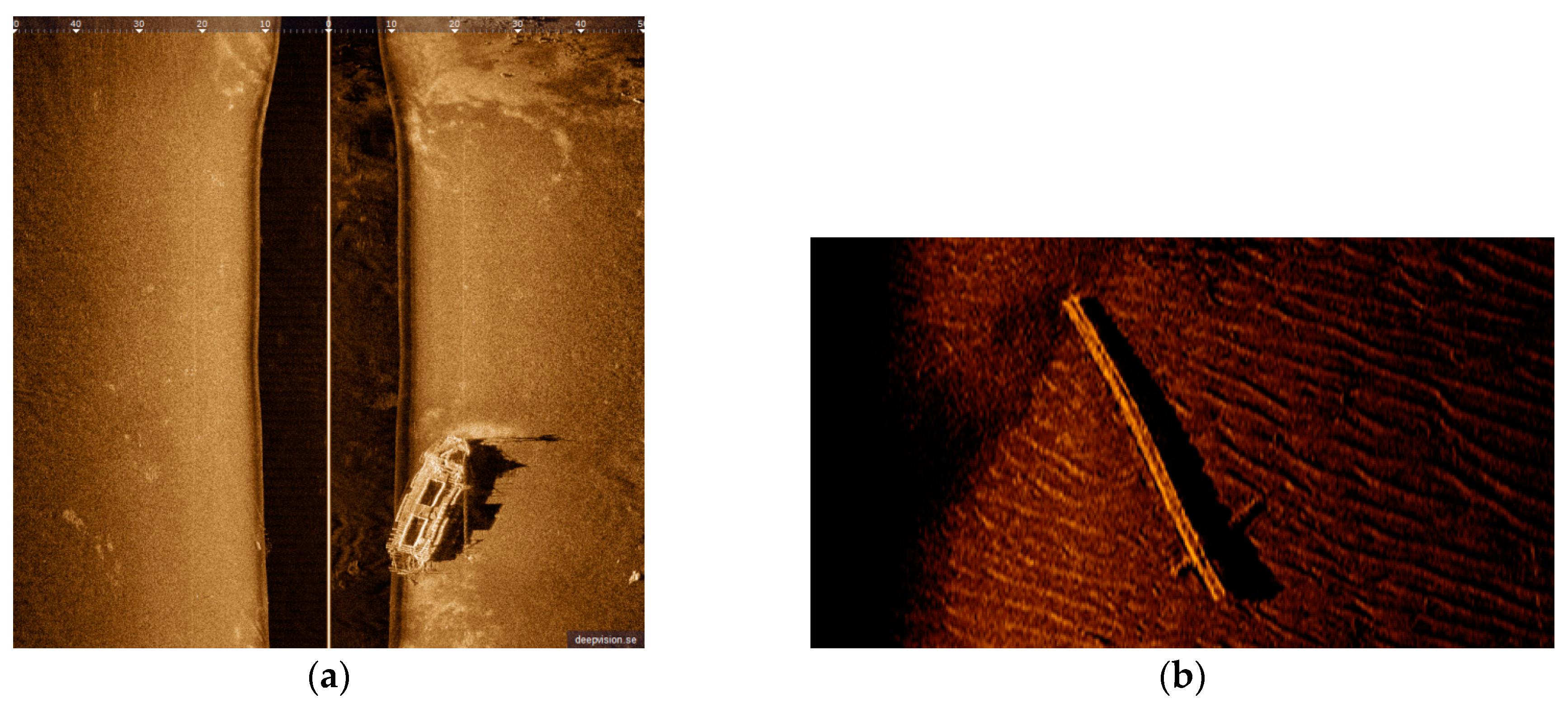
By transmitting and receiving sound via an underwater sonar system, the seafloor terrain and texture information can be extracted with relevant data from the acoustic reflection image of the seabed. High image resolutions are very important for determining if an underwater target is something worth investigating. Two SSS images are used in this work (see
Figure 1).
Figure 1a is of high resolution, whereas
Figure 1b is a low resolution SSS image. Actually, the DE340D SSS (Deep VisionAB company, Linköping, Sweden), the 3500 Klein SSS (Klein Marine System, Inc., Salam, MA, USA), and the Blue View P900-90 2D FLS (Teledyne BlueView, Bothell, WA, USA), all will be employed in our “Smart and Networking Underwater Robots in Cooperation Meshes”-SWARMs European project, that is the reason why we perform feature detection on these sonar images. DE340D SSS is a product of the Deep VisionAB company(Linköping, Sweden) [
40], working at the frequency of 340 kHz with optimized resolution of 1.5 cm. The beam reaches from 15 to 200 m and the maximum operation depth is 100 m. The size of the converted
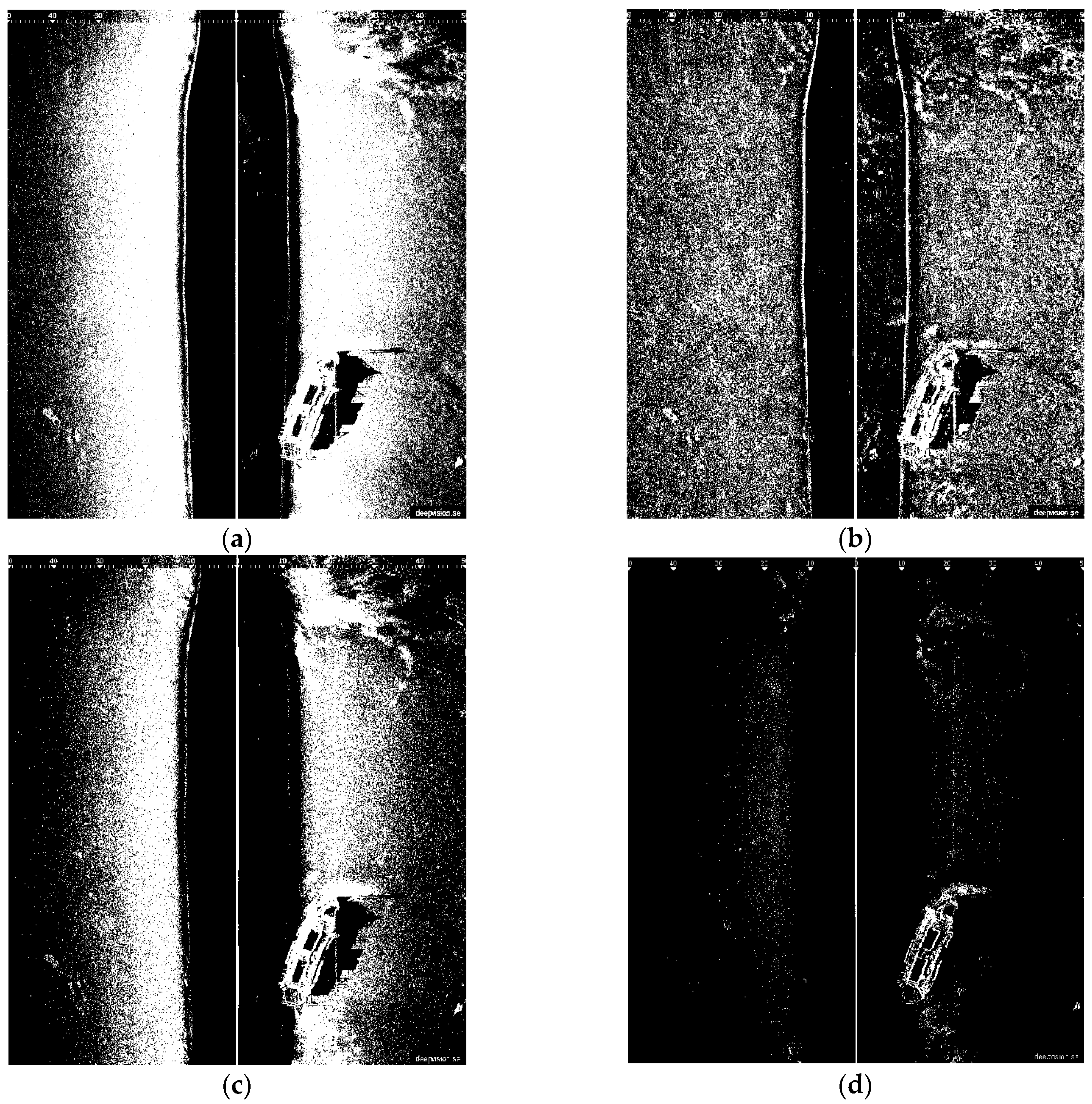
Figure 1a is 800 × 800 = 640,000 pixels. Due to the impact of sediment and fishes, many small bright spots appear in sonar images. The area size of these background spots is usually smaller than 30 pixels, and their gray level is similar to that of certain areas of foreground object. When using the traditional TSM to separate the foreground object, in this case a shipwreck, it can be found that most of these spots are still retained in the segmentation results. To solve this problem, an improved Otsu method is proposed that constrains the search range of the ideal segmentation threshold to separate the foreground object inside the sonar imagery.
It is typical for SSS images to show a vertical white line appearing in the center, indicating the path of the sonar. A dark vertical band on both sides represents the sonar return from the water-column area. Notice that this band has no equal width, and is curved in some parts. The distance from the white line to the end of the dark area is equivalent to the depth to the sea bottom below the sonar device. The seabed is imaged on either side, corresponding to port-side and starboard-side views. Bright areas indicate ascending ground, while dark areas correspond to descending regions or shadows produced by objects, vegetation or rocks. The length of a shadow can be used to calculate the height of an object.
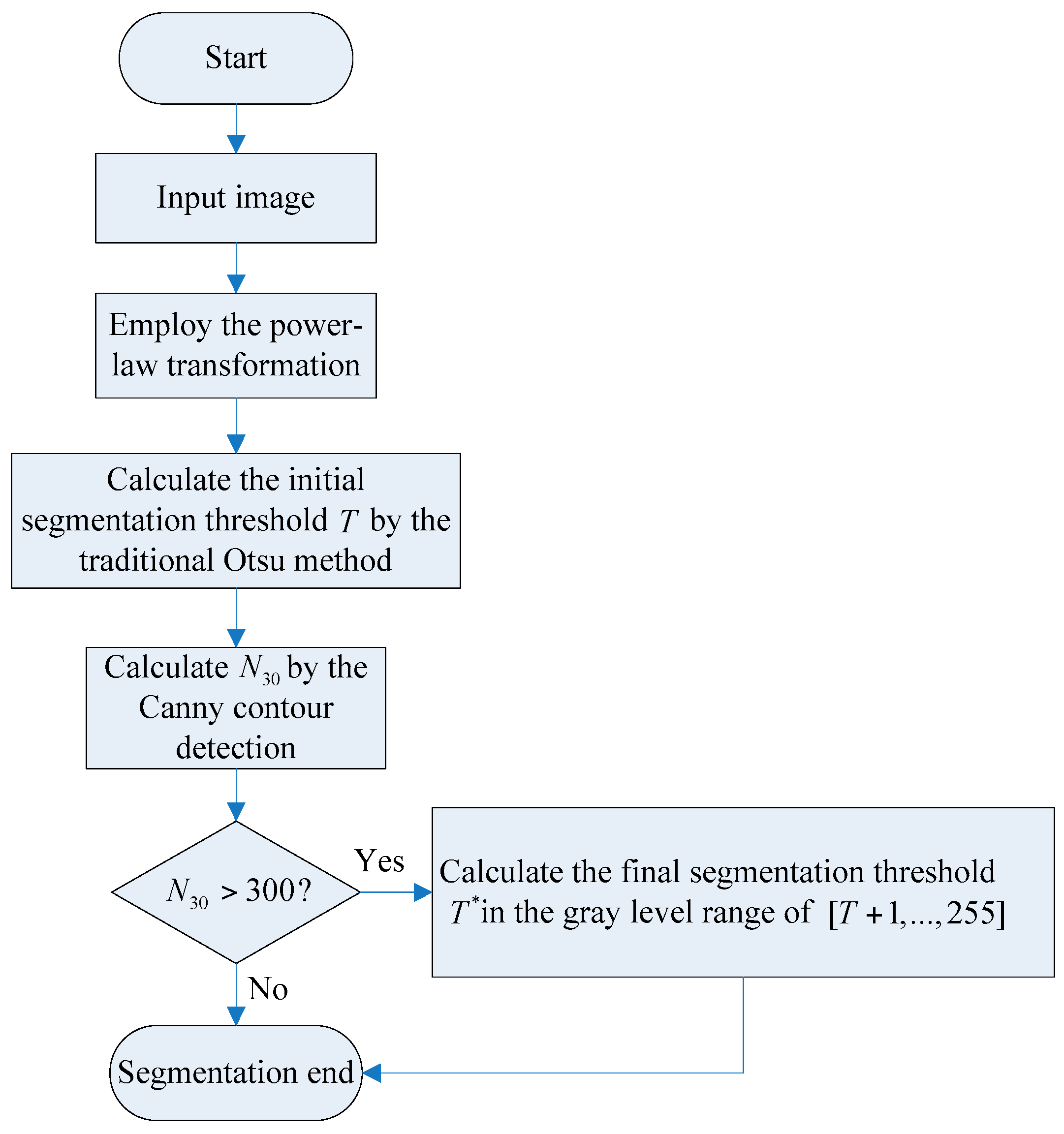
3.2. The Proposed Improved Otsu TSM Algorithm
When using the traditional TSM to separate the foreground object, in this case a shipwreck, most of the background spots are still retained in the segmentation results. To solve this problem, an improved Otsu TSM is presented that constrains the search range of the ideal segmentation threshold to extract the foreground object inside the image. Since the area size of the background spots, shown in
Figure 1a, is usually no bigger than 30 pixels, the parameter
N30 has been defined as the number of contours to be found with an area size smaller than 30 pixels. The procedure of the improved Otsu approach is illustrated in
Figure 2. At first, the traditional Otsu method [
42] is used to calculate the initial segmentation threshold
T. Then, the Moore Neighbor contour detection algorithm [
43,
44] is employed to compute
N30. If
N30 > 300, (64,000/30 × 300 = 71.1:1), it means that there are still many small bright spots remaining in the segmentation result, and the threshold needs to be improved. The final segmentation threshold
T* can be calculated as explained further on. If
N30 ≤ 300, the final segmentation threshold
T* is set as the initial segmentation threshold
T, and segmentation is finished. Notice that both values,
N30 and 300 should be changed depending on the characteristics of the used sonar images.
In the gray level range of one plus the initial segmentation threshold
T calculated by the traditional Otsu method to the gray level of 255, denoted as [
T + 1,…,255], the number of pixels at gray level
i is denoted by
ni, and the total number of pixels is calculated by:
The gray level histogram is normalized and regarded as a probability distribution:
Supposing that the pixels are dichotomized into two categories
C0 and
C1 by a threshold
T*. The set
C0 implies the background pixels with a gray level of [
T + 1, …,
T*], and
C1 means those pixels of foreground object with a gray level of [
T + 1, …, 255]. The probabilities of gray level distributions for the two classes are the following:
w0 is the probability of the background and
w1 is the probability of the object:
The means of the two categories
C0 and
C1 are:
The total mean of gray levels is denoted by:
The two class variances are given by:
The within-class variance is:
The between-class variance is:
The total variance of the gray levels is:
The final threshold
T* is chosen by maximizing the between-class variance, which is equivalent to minimizing the within-class variance, since the total variance, which is the sum of the within-class variance
and the between-class variance
, is constant for different partitions:
3.5. TSM Results for Forward-Looking Sonar Image
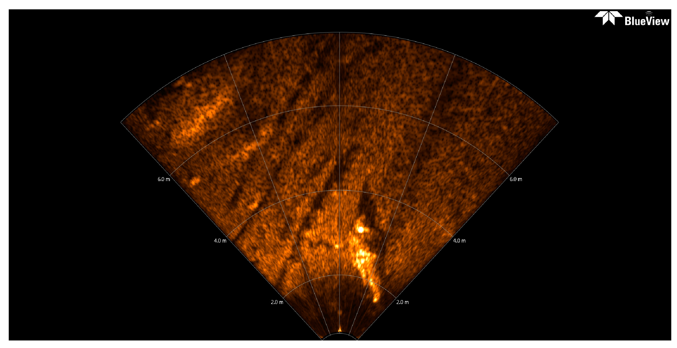
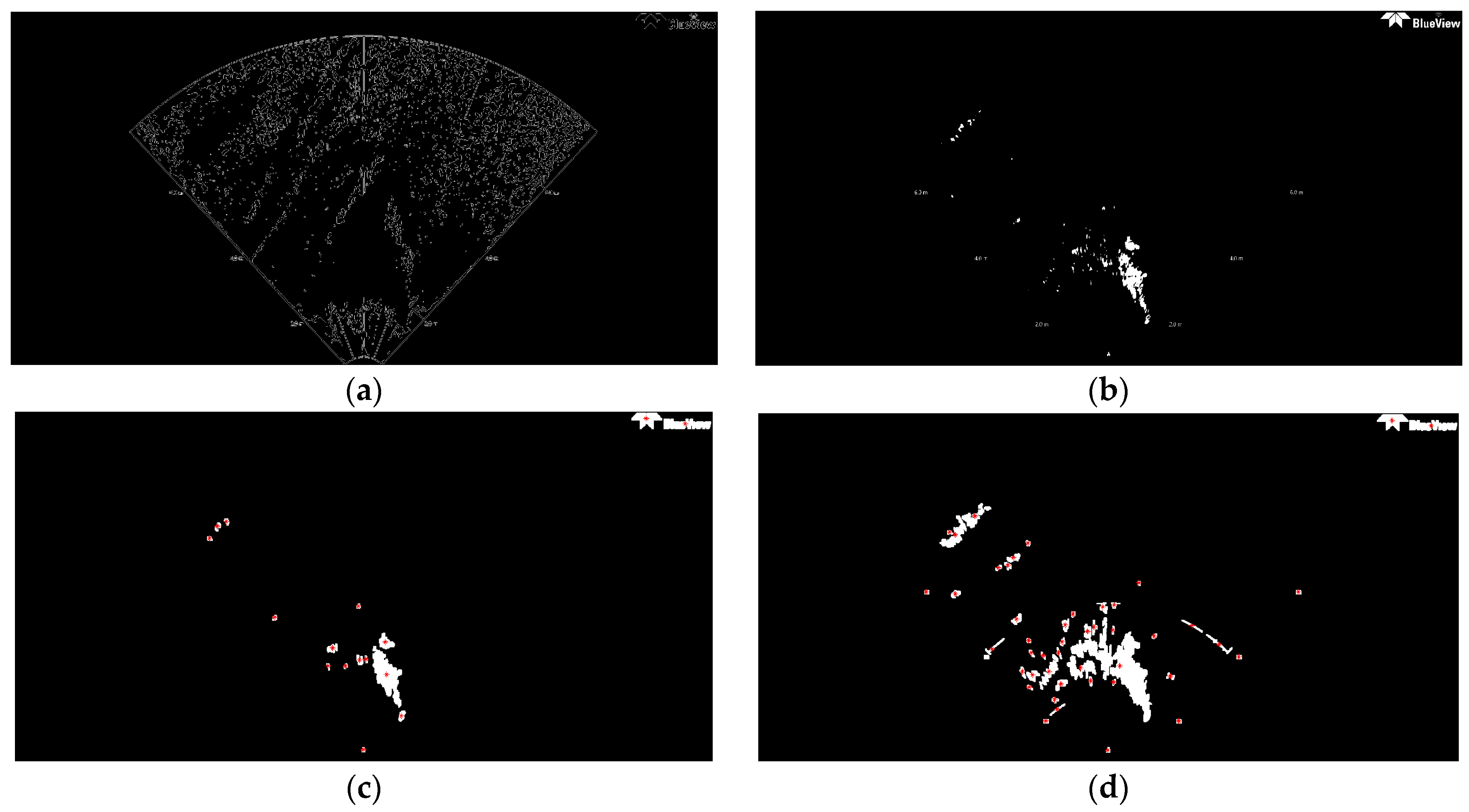
Usually, a preliminary mission of AUV is data collection, generally accomplished by means of SSS or multibeam echosounder, another key issue is to ensure the safety of the AUV. For the purpose of avoiding obstacles, the AUV could be equipped with a forward-looking sonar (FLS) to sense the working environment at a certain distance in the direction of navigation. The FLS platform emits a short acoustic pulse in forward direction on a horizontal sector of around 120°, and on a vertical sector from 15° to 20°. The original FLS imagery used here (see
Figure 8) is provided by Desistek Robotik Elektronik Yazilim company (Ankara, Turkey) [
48]. It is recorded with the Blue View P900-90 2D Imaging Sonar, which has a 90° horizontal field of view, and works at a frequency of 900 kHz. Its update rates are up to 15 Hz, the scanning range is 100 m, and its resolution is 2.51 cm.
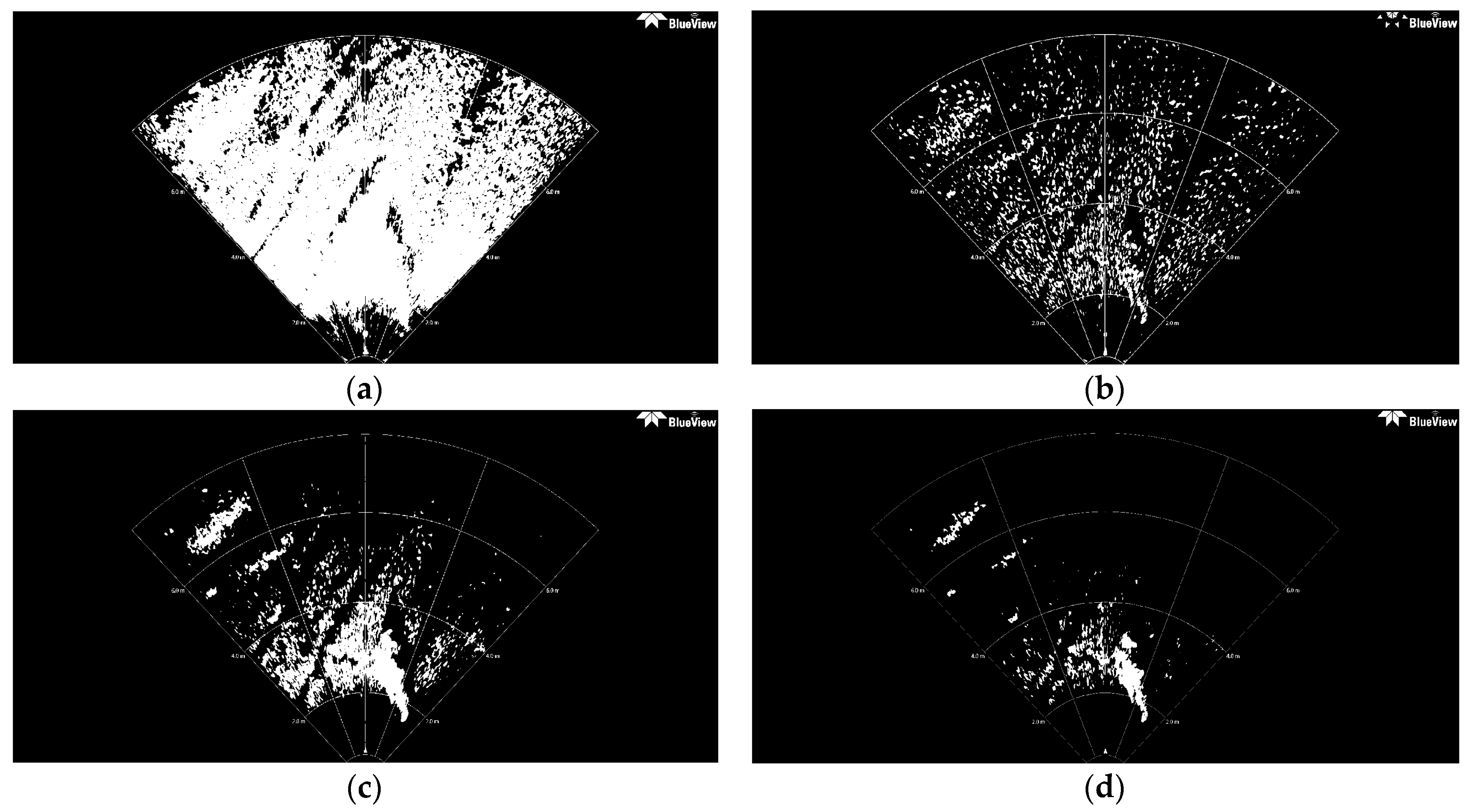
The size of the converted FLS imagery is 1920 × 932 = 1,789,440 pixels, the area size of the background spots is usually fewer than 40 pixels, with gray levels similar to those of certain areas of the foreground objects. In this case, N40 is defined as the number of contours which area size is smaller than 40 pixels, and it is computed by the Canny contour detection algorithm. If N40 > 600, (1,789,440/40 × 600 = 74.6:1), this assigned threshold 74.6 is higher than that of 71.1 for the former high resolution SSS image of the ship, that is because the black background proportion in this presented FLS image is higher than that in that SSS image. This means that there are many small bright spots still left in the segmentation result.
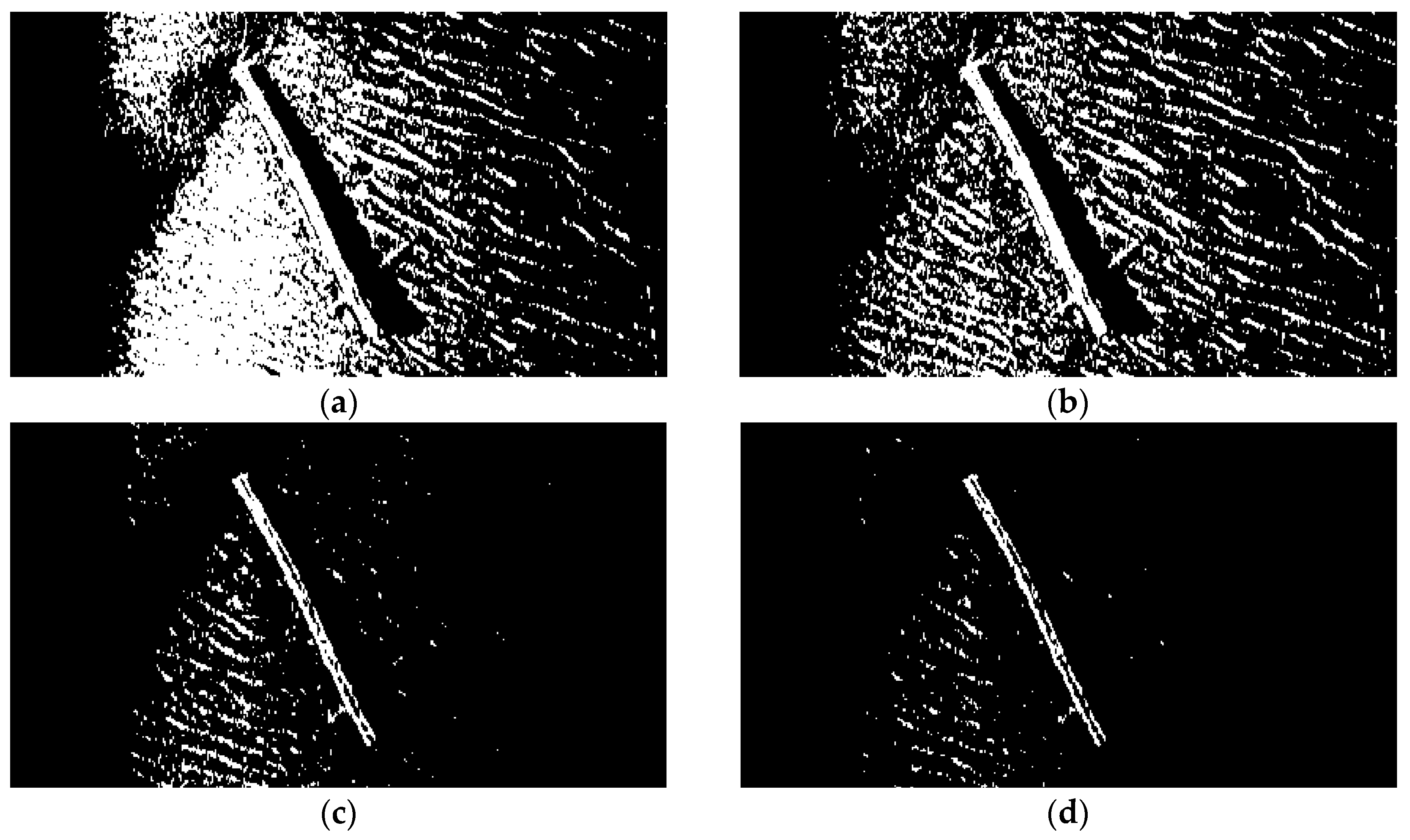
The initial FLS image in
Figure 8 has been segmented with the traditional Otsu method, the local TSM, the iterative TSM, the maximum entropy TSM and our method, respectively. The results of these segmentations are shown in
Figure 9 and
Figure 10.The initial segmentation threshold
T obtained via the traditional Otsu method is 0.1176. In
Figure 10a, the parameter
N40 calculated from the above Canny edge detection algorithm is 1341, which is bigger than 600. Thus, our improved Otsu TSM has been applied, and the segmentation result is shown in
Figure 10b, with the final threshold
T* of 0.5412. The morphological operations for computing the centroids of every segmented region within the body are similar to that of the ship. Only in step 1, the parameter is set to 40, in order to remove all connected components that have fewer than 40 pixels. Besides, in step 3, it applies dilation two times.
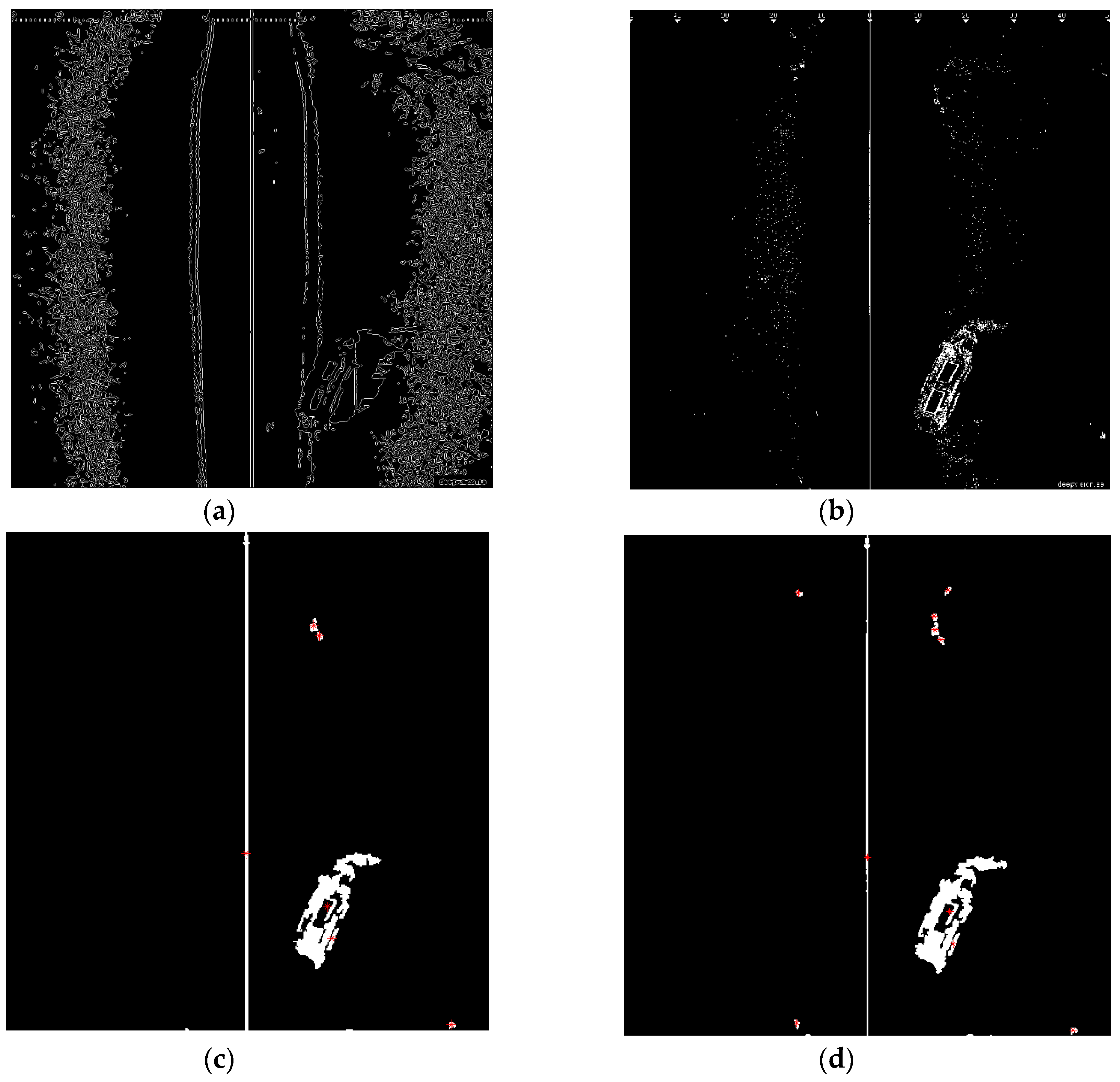
The red stars ‘*’, shown in
Figure 10c, stand for the centroids for each contiguous region or connected component in this image. The centroid coordinates of every connected region within the foreground object are (949.8, 662.9), (966.9, 660.6), (1021.2, 615.7), (1024.1, 703) and (1065.5, 811.3), and will be used as landmark points in the further simulation test of an AEKF-based SLAM loop mapping. So, the center centroid of the body is (1005.5, 690.7), which is calculated as the average of the above five centroids. The same morphological operations for marking the feature centroids is employed on the segmentation result of the maximum entropy TSM, shown in
Figure 10d. The confusion matrices of the real body centroids and the ones detected by the improved Otsu TSM on the one hand and the maximum entropy TSM on the other hand are shown in the following
Table 7 and
Table 8, respectively.
As for the former SSS images, we calculate the FPR and PPV indicators:
In this case, the FPR and the precision value are:
As can be seen, also for the FLS images, similar performance is achieved with the improved Otsu TSM. The FPR value is 1.8 times lower and the precision is seven times higher, even better than for the SSS images, which means that, the lower the image quality is, the better the detection performance for important features. Besides, three real body centroids are not detected at all by the maximum entropy TSM. In general, in all SSS and FLS images presented in this work, the proposed improved Otsu TSM has much lower FPR and much higher precision rate on the detected feature centroids than those values of the maximum entropy TSM.
Finally, again the computational cost of the proposed improved Otsu TSM is compared with the above indicated four conventional segmentation methods on executed
Figure 8 and the results are shown in
Table 9. It is higher than for the traditional Otsu TSM, the local TSM and the iterative TSM, but nearly one third of the time needed by the maximum entropy TSM, Instead, much better detection rates are achieved.
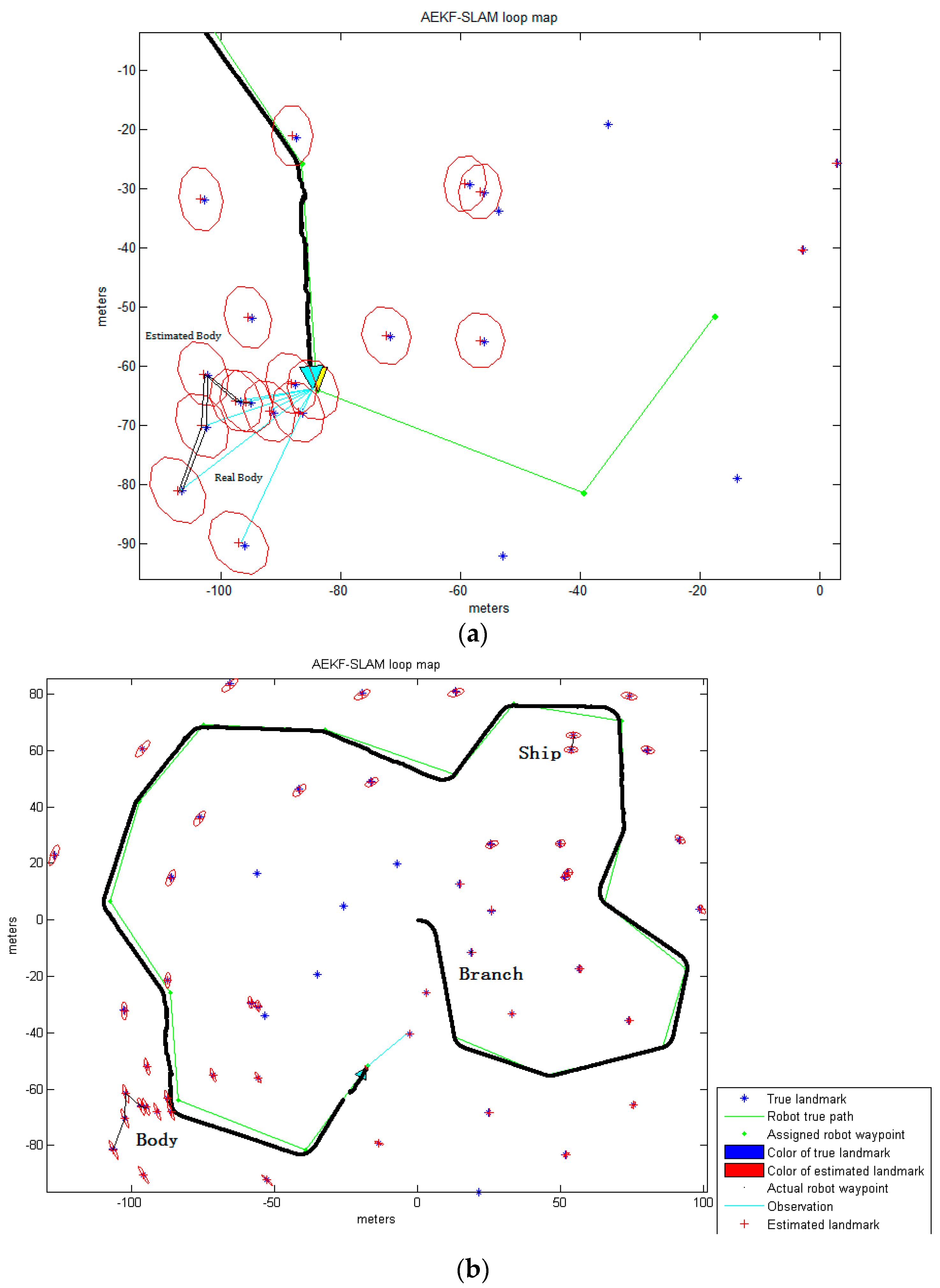
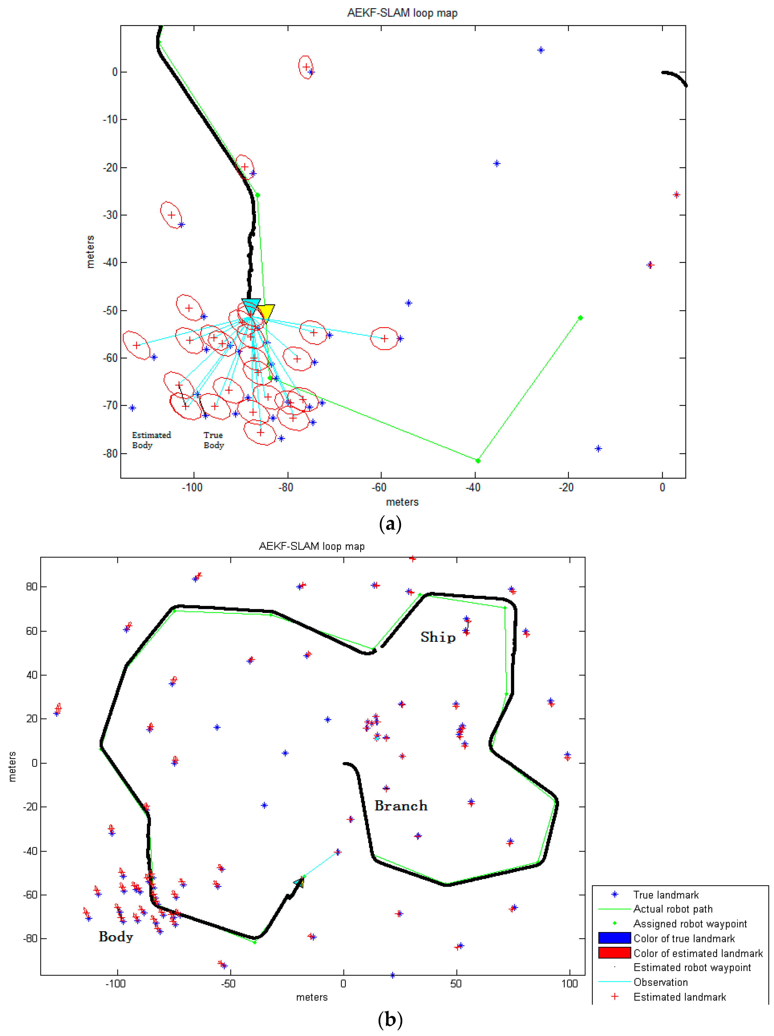
In general, the improved Otsu TSM constrains the search range of the ideal segmentation threshold, and combined with the contour detection algorithm, the foreground object of interest, a ship, a branch and a body have been separated more accurately, in sonar images of very different resolutions and qualities, with a low computational time. Compared with the maximum entropy TSM, which has the highest segmentation accuracy among the four conventional segmentation approaches compared above, our improved Otsu TSM just needs half of the processing time for segmenting the ship in the high resolution SSS image. Regarding the branch in the low resolution SSS image, our method consumes two thirds of the time, and for the body in the presented FLS image, it only spends one third of the computational time used by the maximum entropy TSM. As a result, the improved Otsu TSM achieves precise threshold segmentation performances for underwater feature detection at a fast computational speed. Since the computational time of the improved Otsu TSM is very short, it achieves real time results which can be used afterwards for underwater SLAM. The centroids that have been calculated for the different objects will be used as landmark points in the following AEKF-SLAM loop map simulation. Moreover, compared to the traditional Otsu method, the presented approach could retain more complete information and details of objects after segmentation, also the holes and gaps in objects are reduced.


