
Spectral Characterization of a Prototype SFA Camera for Joint Visible and NIR Acquisition


Abstract
:
1. Introduction
2. Description of the System
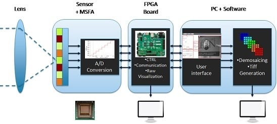
2.1. Camera Architecture
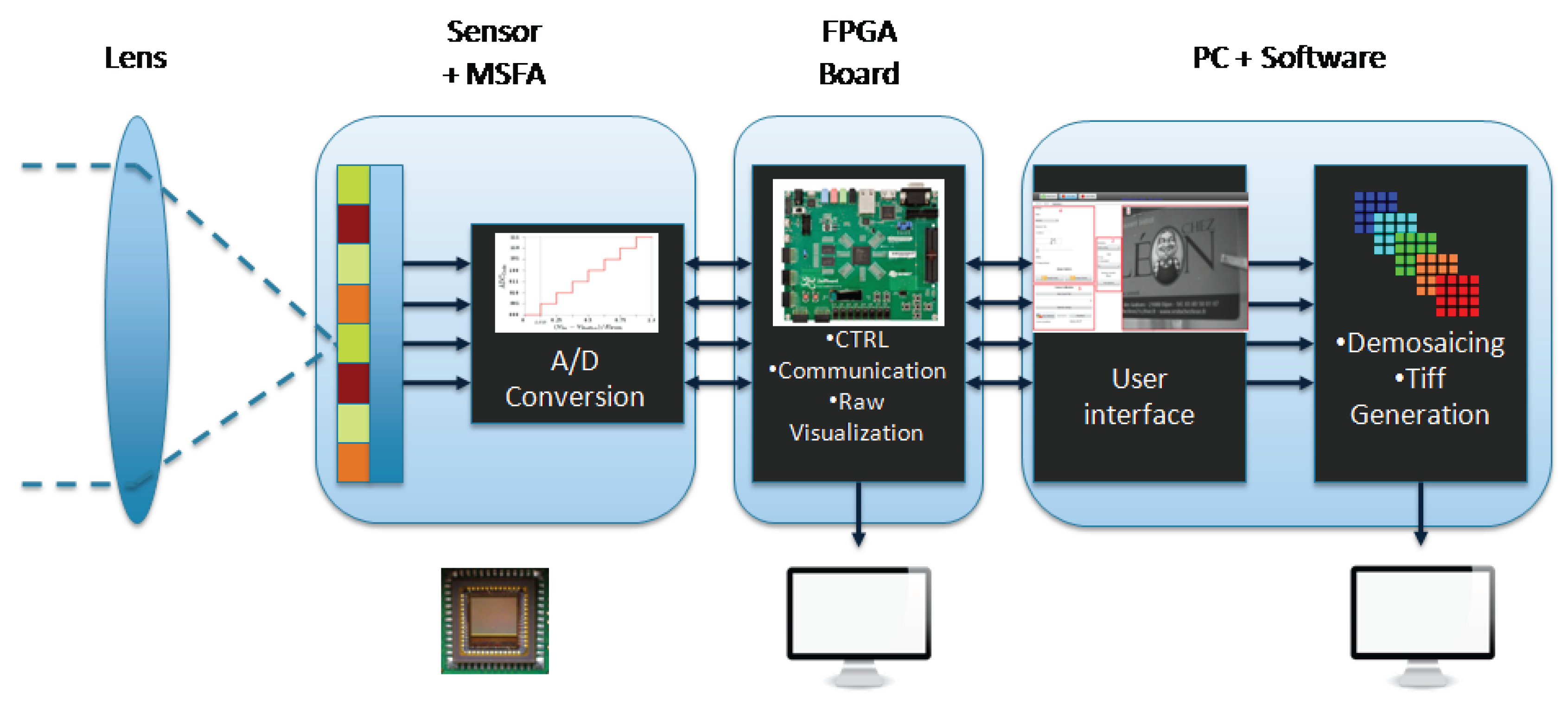
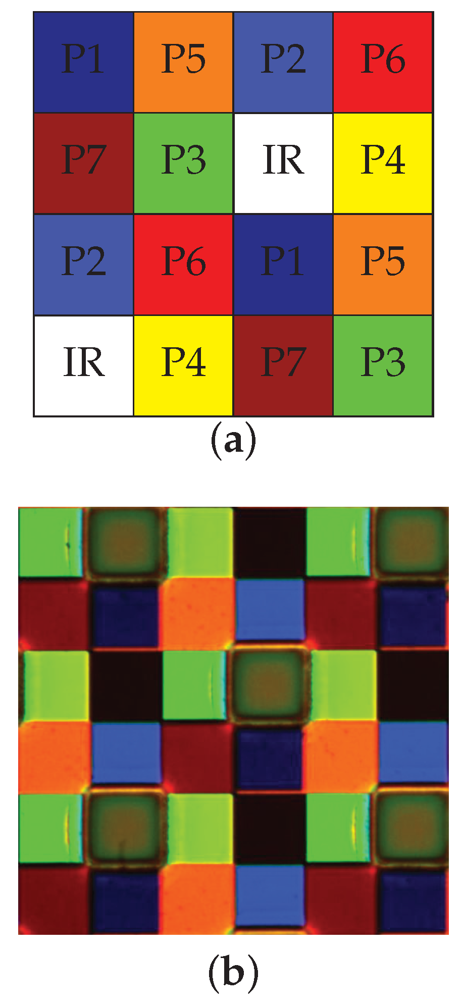
2.2. Spatial Arrangement
3. Spectral Characterization
3.1. Pre-Processing
3.1.1. Dark Master
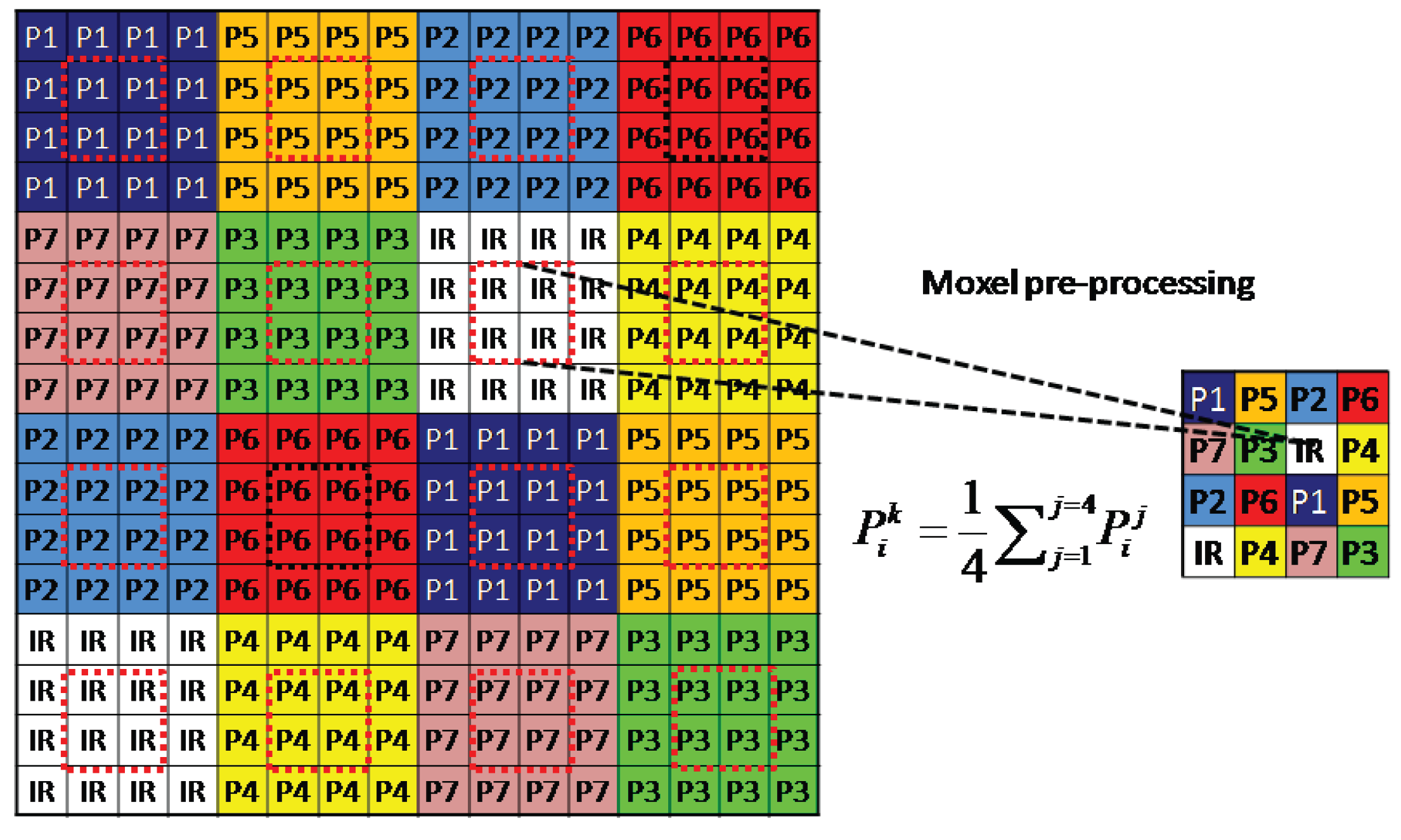
3.1.2. Downsampling
3.2. Spectral Sensitivities
3.2.1. Spectral Characterization
- Create a Dark Master image for the given exposure time as described in Section 3.1.1.
- Downsample and pre-process the images as described in Section 3.1.1 and Section 3.1.2.
- Capture 2 sets of images of monochromatic light.
- Average the 2 image sets.
- Select a square of 84 pixels at the center of each image, where a small angle inaccuracy would be negligible and where the monochromatic light is assumed to be uniform according to the specification of our devices, with a large security margin.
- Sort out pixels by filter type and apply light source monochromator calibration to the data.
- Average the curves from the 84 × 84 pixels.
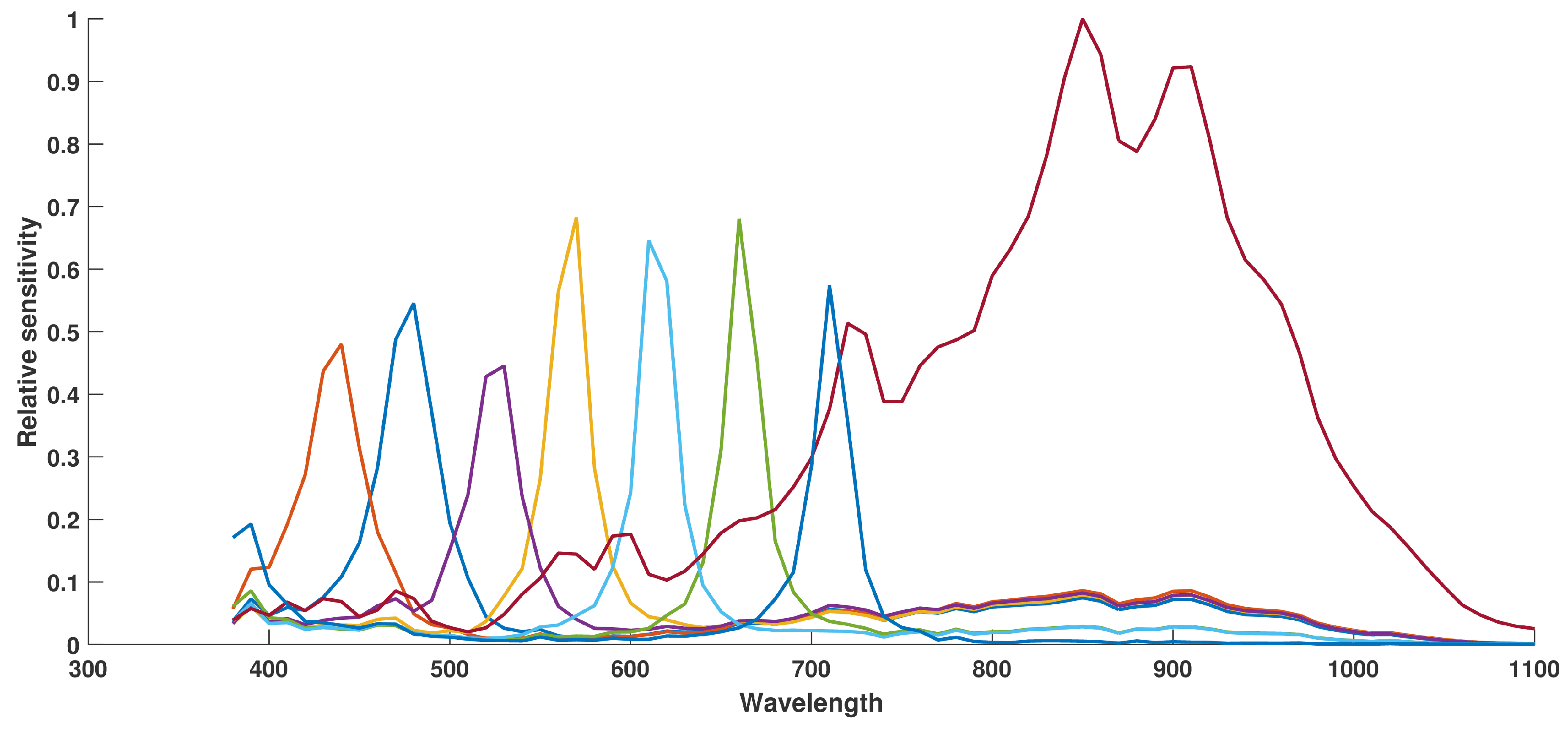
- Normalize the curve over the highest number. By doing that, we preserve the ratio of efficiencies by channel, assuming a linear sensor.
3.2.2. Analysis
4. Multispectral Imaging
4.1. Energy Balance
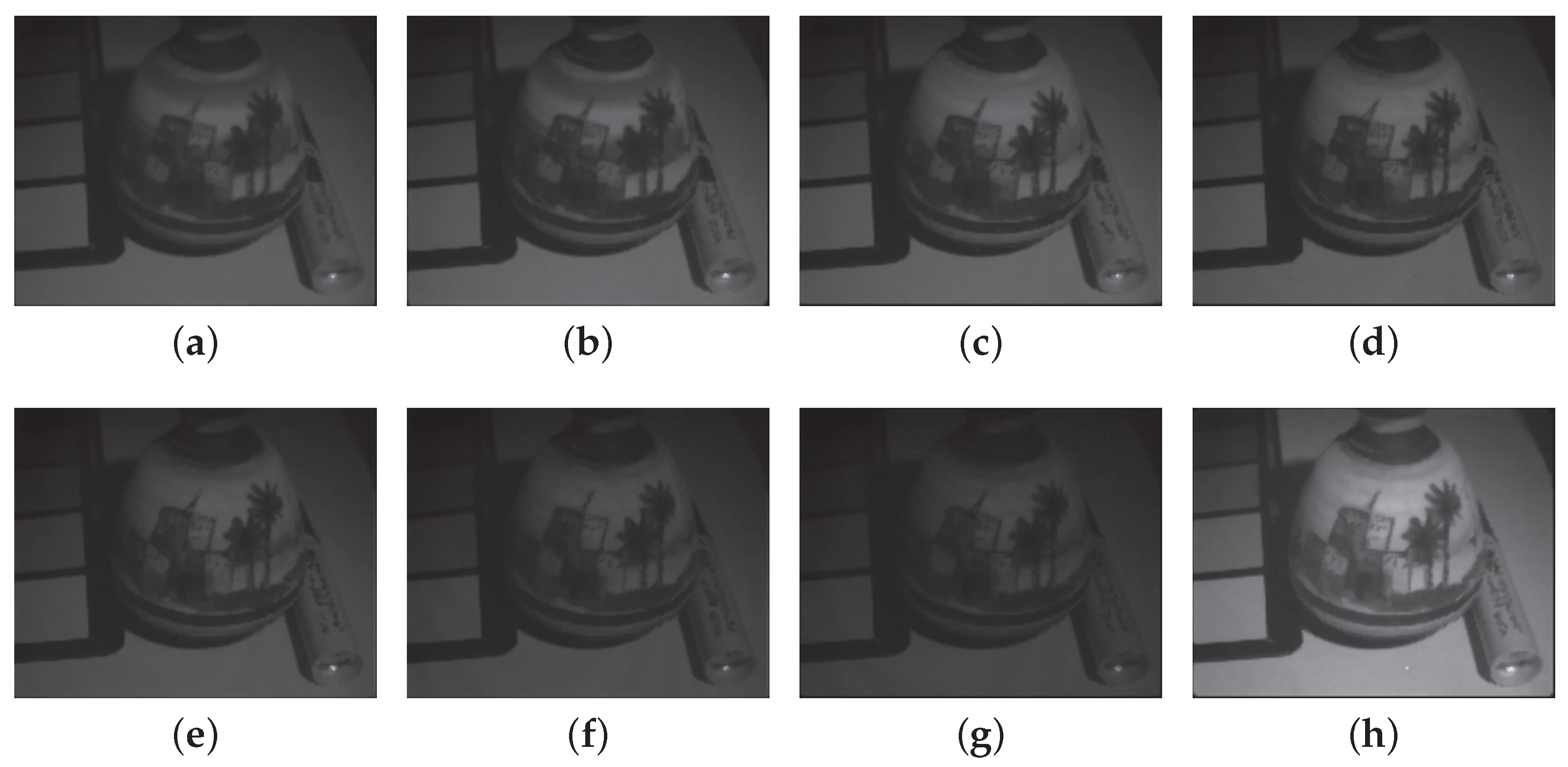
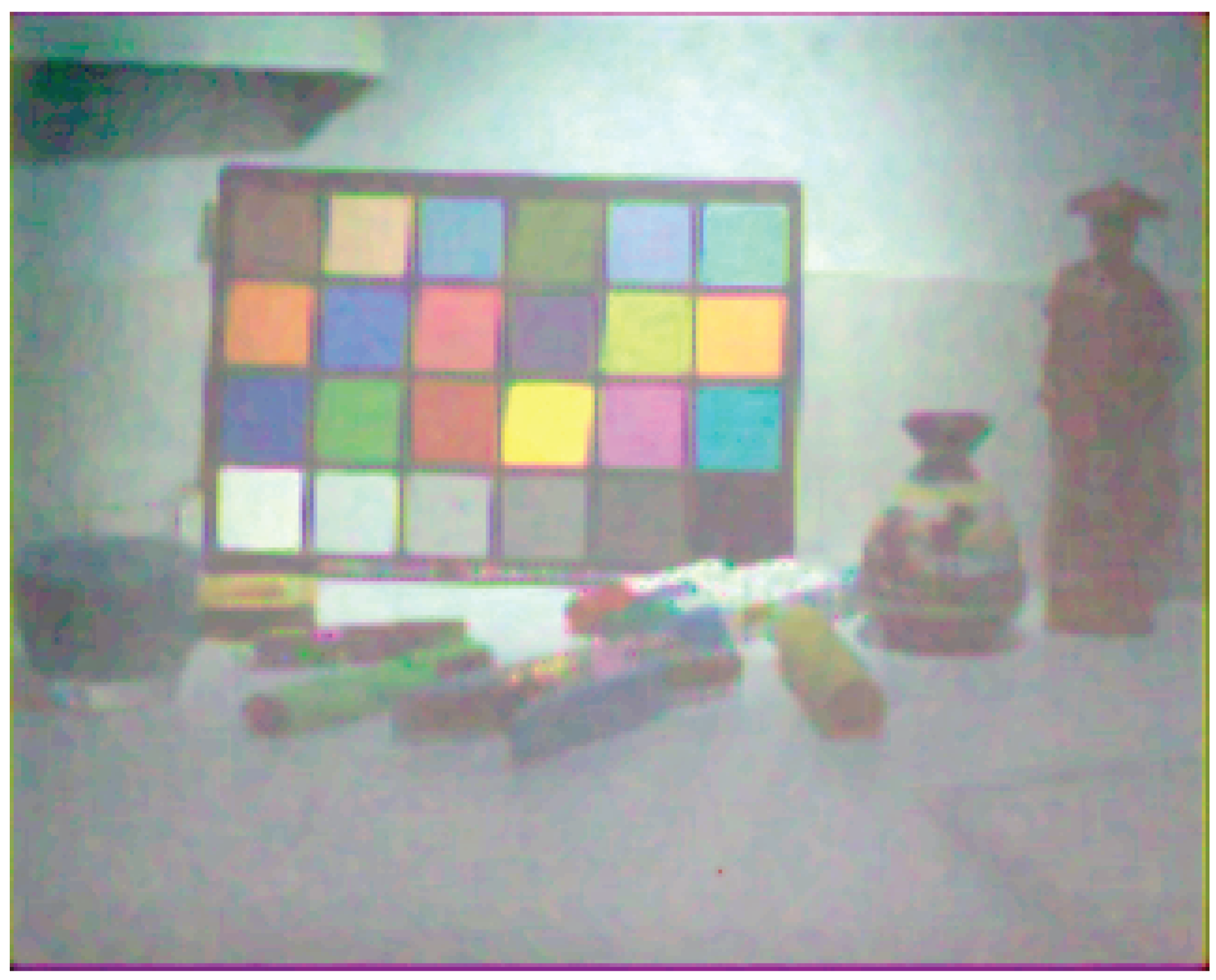
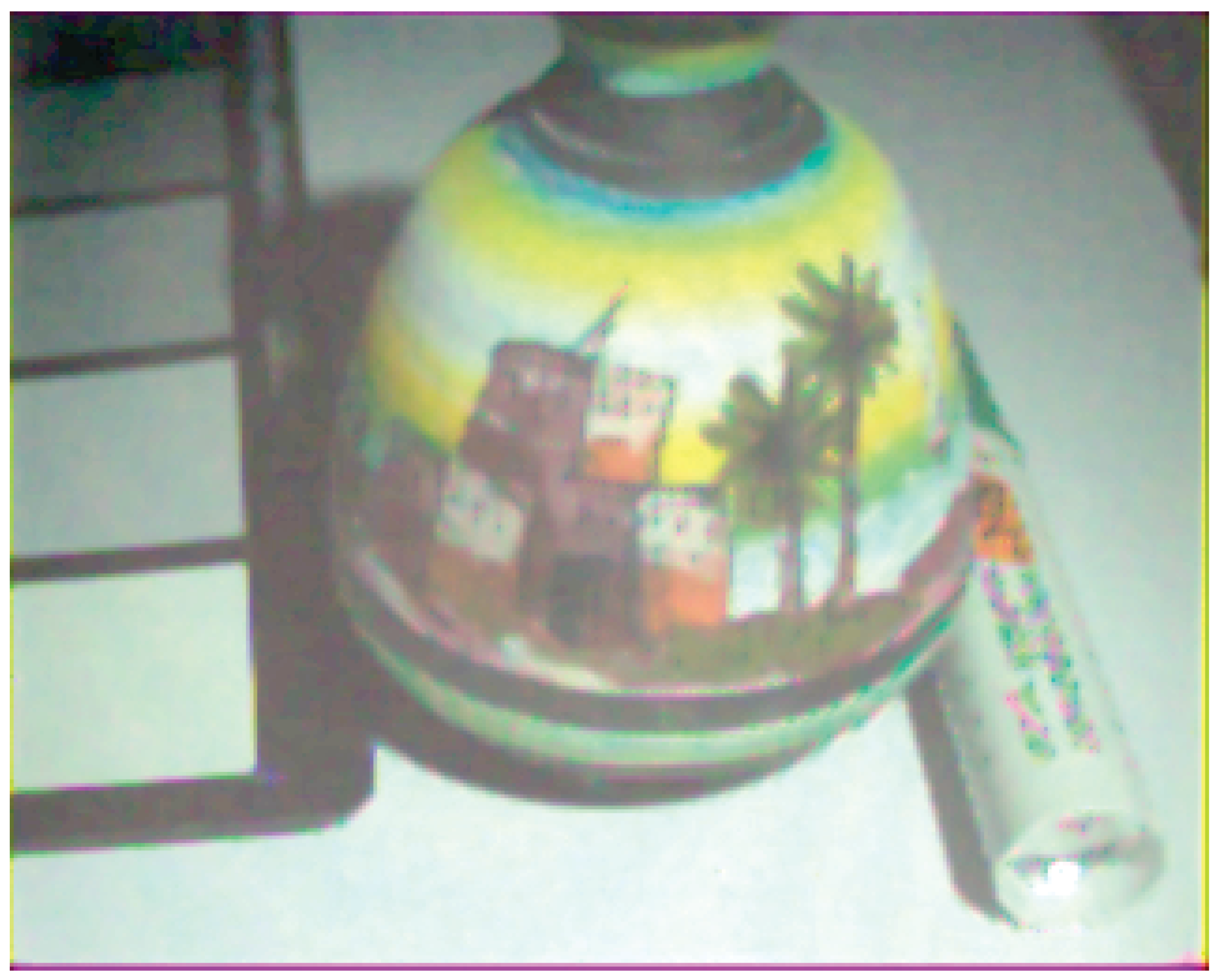
4.2. Images Acquired
5. Conclusions
Supplementary Materials
Acknowledgments
Author Contributions
Conflicts of Interest
Appendix A
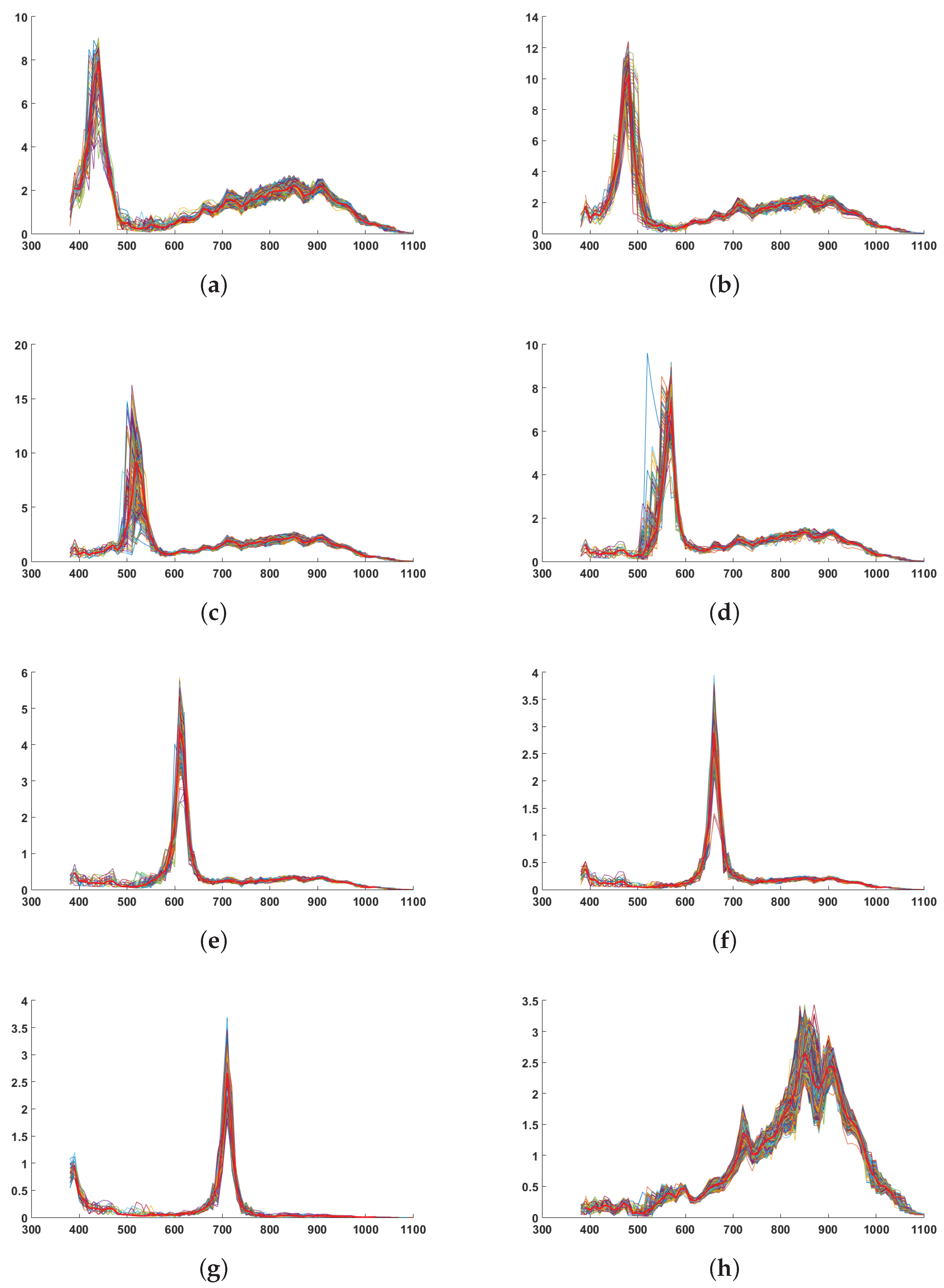
- We observe a large offset common to all the channels in shorter wavelengths.
- We observe a large bandpass behavior in the NIR for the bands that have peaks in the visible (Figure A1a,g). We observe that the behavior of some pixels are quite different in this part.
- We observe that the channel that have peak in the NIR (Figure A1h) has a huge variance compared to visible spectral bands.
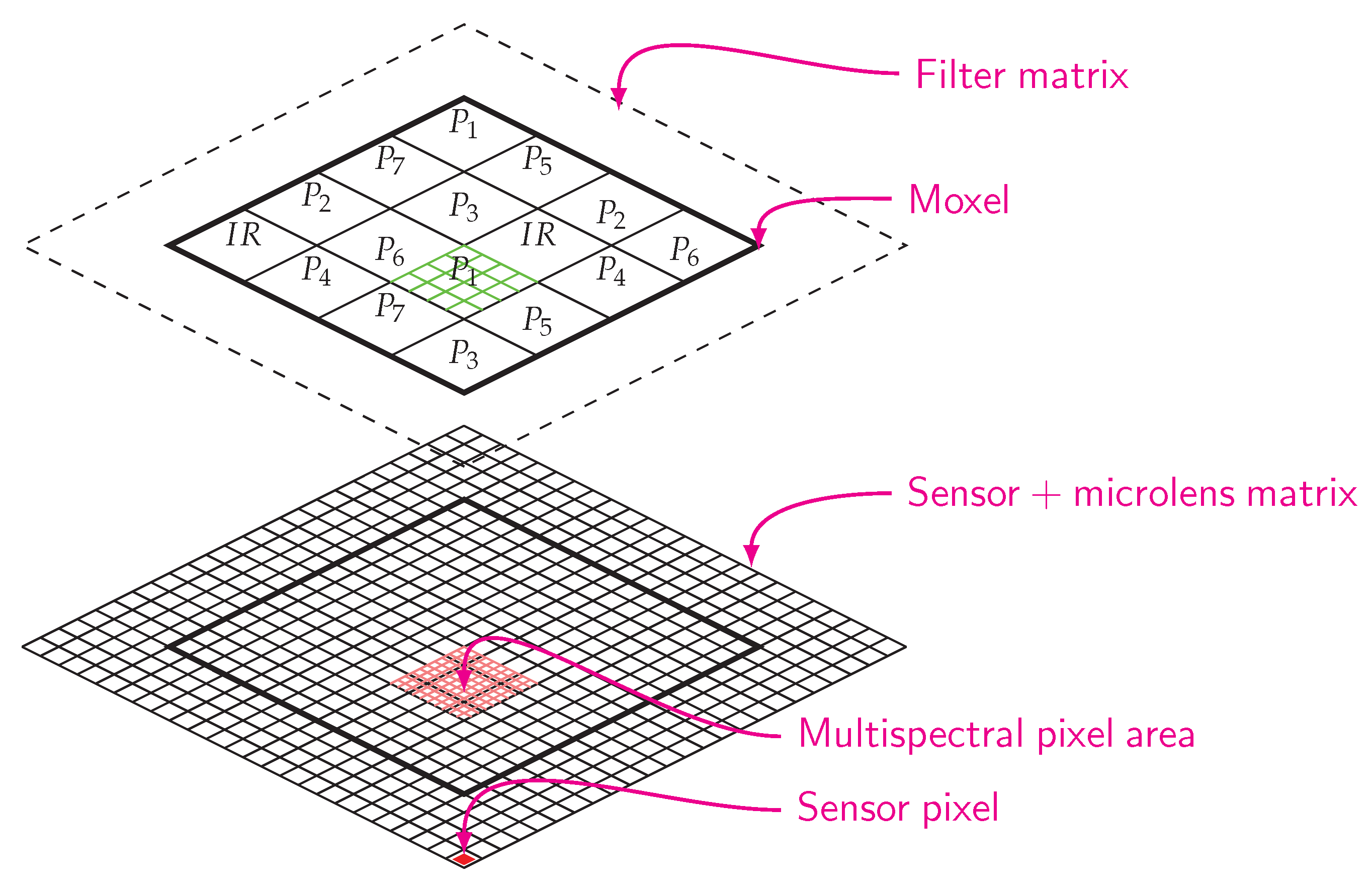
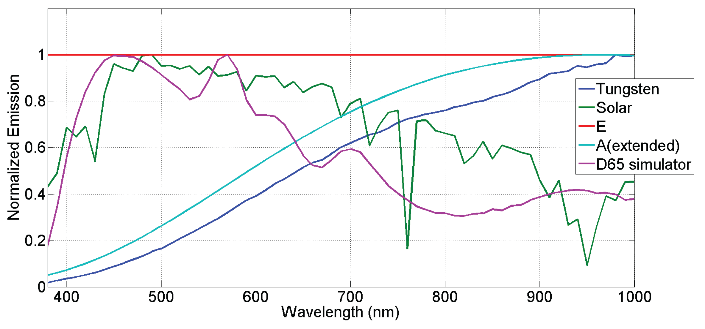
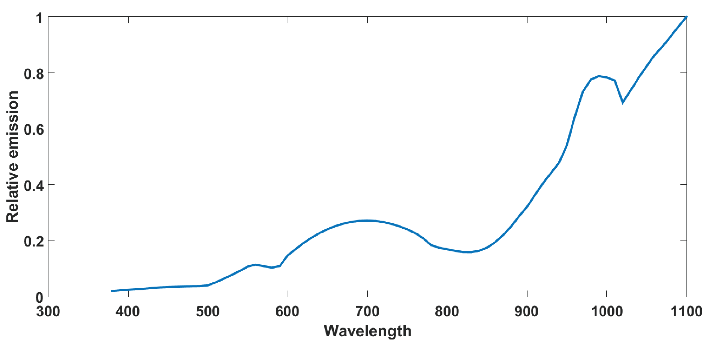
- The large offset common to all channels is higher for the short wavelengths. This is related and proportional to the weakness of the light source used in the experiment, shown in Figure A2, in this range of wavelengths. We argue this would be a multiplicative contribution of the dark noise while accounting for the energy of the light source. This can be corrected by applying a dark noise correction to all acquired images.
- According to the specific behavior in the NIR sensitivity of the visible bands, we argue that this is directly related to the proximity of an infrared pixel. This is induced by an inaccuracy in NIR filter realization as can be seen in Figure 4b. The NIR filter is overlapping on the connected cells. In addition, the filter layer is positioned at some distance of the micro-lenses, which creates cross-talk on neighbor pixels. Without any pre-processing, we observed that the bands of the visible domain transmit a part of the intensity range in the NIR. The shape of (Figure A1a,g) response curves seemed to be rather consistent with the NIR channel itself. In addition, the light that hits the bands , , and appeared to pass through the wavelength range of 780–1100 nm, and in a greater magnitude compared to bands and . We also observed that was very poorly affected by this phenomenon due to its position in the mosaic. This behavior is explained by the fact that the bands located physically closer to the pixels of the NIR band are affected by it. This effect can be partially corrected by selecting pixels at the center of each filters and discarding the others.
- The big variance in the NIR channel is due to the process of thin layer deposition, which is different from the micro-/nano-etching of the visible bands. Different behaviors can be observed sliding from a high sensitivity in the visible to less. This behavior resembles variation of transmittance filters according to a gradient thin layer deposition. Indeed, we could explain this behavior by a graduated thickness of the NIR filter. This effect can be partially corrected by selecting the pixels at the center of the NIR filters, where the thin layer is supposed flat and uniform and discarding the others.


References
- Kong, L.; Sprigle, S.; Yi, D.; Wang, F.; Wang, C.; Liu, F. Developing handheld real time multispectral imager to clinically detect erythema in darkly pigmented skin. Proc. SPIE 2010, 7557. [Google Scholar] [CrossRef]
- Shrestha, S.; Deleuran, L.C.; Olesen, M.H.; Gislum, R. Use of Multispectral Imaging in Varietal Identification of Tomato. Sensors 2015, 15, 4496–4512. [Google Scholar] [CrossRef] [PubMed]
- Smith, M.O.; Ustin, S.L.; Adams, J.B.; Gillespie, A.R. Vegetation in deserts: I. A regional measure of abundance from multispectral images. Remote Sens. Environ. 1990, 31, 1–26. [Google Scholar] [CrossRef]
- Park, B.; Lawrence, K.C.; Windham, W.R.; Smith, D.P. Multispectral imaging system for fecal and ingesta detection on poultry carcasses. J. Food Process Eng. 2004, 27, 311–327. [Google Scholar] [CrossRef]
- Vagni, F. Survey of Hyperspectral and Multispectral Imaging Technologies (Etude sur les Technologies D’imagerie Hyperspectrale et Multispectrale). Available online: https://www.google.com/url?sa=t&rct=j&q=&esrc=s&source=web&cd=2&ved=0ahUKEwjt4afg3MfNAhUBrI8KHYGuBMEQFggnMAE&url=http%3A%2F%2Fwww.dtic.mil%2Fcgi-bin%2FGetTRDoc%3FAD%3DADA473675&usg=AFQjCNFIYZvH_ms6uCrogY-vBniY9JM9wA&bvm=bv.125596728,d.dGo&cad=rjt (accessed on 1 April 2016).
- Bayer, B.E. Color Imaging Array. U.S. Patent 3,971,065, 20 July 1976. [Google Scholar]
- Vrhel, M.J.; Trussell, H.J. Filter considerations in color correction. IEEE Trans. Image Process. 1994, 3, 147–161. [Google Scholar] [CrossRef] [PubMed]
- Vrhel, M.J.; Trussell, H.J. Optimal color filters in the presence of noise. IEEE Trans. Image Process. 1995, 4, 814–823. [Google Scholar] [CrossRef] [PubMed]
- Barnard, K.; Funt, B. Camera characterization for color research. Color Res. Appl. 2002, 27, 152–163. [Google Scholar] [CrossRef]
- Quan, S. Evaluation and Optimal Design of Spectral Sensitivities for Digital Color Imaging. Ph.D. Thesis, Rochester Institute of Technology, New York, NY, USA, April 2002. [Google Scholar]
- Sadeghipoor Kermani, Z.; Lu, Y.; Süsstrunk, S. Optimum Spectral Sensitivity Functions for Single Sensor Color Imaging. Proc. SPIE 2012. [Google Scholar] [CrossRef]
- Wang, X.; Pedersena, M.; Thomas, J.B. The influence of chromatic aberration on demosaicking. In Proceedings of the 2014 5th European Workshop on Visual Information Processing (EUVIP), Paris, France, 10–12 December 2014; pp. 1–6.
- Wang, X.; Green, P.J.; Thomas, J.; Hardeberg, J.Y.; Gouton, P. Evaluation of the Colorimetric Performance of Single-Sensor Image Acquisition Systems Employing Colour and Multispectral Filter Array. In Proceedings of the 5th International Workshop, CCIW 2015, Saint Etienne, France, 24–26 March 2015.
- Li, X.; Gunturk, B.; Zhang, L. Image demosaicing: A systematic survey. Proc. SPIE 2008. [Google Scholar] [CrossRef]
- Ramanath, R.; Snyder, W.E.; Yoo, Y.; Drew, M.S. Color image processing pipeline. IEEE Signal Process. Mag. 2005, 22, 34–43. [Google Scholar] [CrossRef]
- Hagen, N.; Kudenov, M.W. Review of snapshot spectral imaging technologies. Opt. Eng. 2013, 52, 090901. [Google Scholar] [CrossRef]
- Lapray, P.J.; Wang, X.; Thomas, J.B.; Gouton, P. Multispectral Filter Arrays: Recent Advances and Practical Implementation. Sensors 2014, 14, 21626–21659. [Google Scholar] [CrossRef] [PubMed]
- Frey, L.; Masarotto, L.; Armand, M.; Charles, M.L.; Lartigue, O. Multispectral interference filter arrays with compensation of angular dependence or extended spectral range. Opt. Expr. 2015, 23, 11799–11812. [Google Scholar] [CrossRef] [PubMed]
- Vial, B. Study of Open Electromagnetic Resonators by Modal Approach. Application to Infrared Multispectral Filtering. Ph.D. Thesis, Ecole Centrale Marseille, Marseille, France, Decemeber 2013. [Google Scholar]
- Park, H.; Crozier, K.B. Multispectral imaging with vertical silicon nanowires. Sci. Rep. 2013, 3, 2460. [Google Scholar] [CrossRef] [PubMed]
- Najiminaini, M.; Vasefi, F.; Kaminska, B.; Carson, J.J.L. Nanohole-array-based device for 2D snapshot multispectral imaging. Sci. Rep. 2013, 3, 2589. [Google Scholar] [CrossRef] [PubMed]
- Monno, Y.; Kikuchi, S.; Tanaka, M.; Okutomi, M. A Practical One-Shot Multispectral Imaging System Using a Single Image Sensor. IEEE Trans. Image Process. 2015, 24, 3048–3059. [Google Scholar] [CrossRef] [PubMed]
- Murakami, Y.; Yamaguchi, M.; Ohyama, N. Hybrid-resolution multispectral imaging using color filter array. Opt. Expr. 2012, 20, 7173–7183. [Google Scholar] [CrossRef] [PubMed]
- Martínez, M.A.; Valero, E.M.; Hernández-Andrés, J.; Romero, J.; Langfelder, G. Combining transverse field detectors and color filter arrays to improve multispectral imaging systems. Appl. Opt. 2014, 53, C14–C24. [Google Scholar] [CrossRef] [PubMed]
- Geelen, B.; Tack, N.; Lambrechts, A. A compact snapshot multispectral imager with a monolithically integrated per-pixel filter mosaic. Proc. SPIE 2014. [Google Scholar] [CrossRef]
- Wang, X.; Thomas, J.B.; Hardeberg, J.Y.; Gouton, P. Median filtering in multispectral filter array demosaicking. Proc. SPIE 2013. [Google Scholar] [CrossRef]
- Wang, X.; Thomas, J.B.; Hardeberg, J.Y.; Gouton, P. Discrete wavelet transform based multispectral filter array demosaicking. In Proceedings of the Colour and Visual Computing Symposium (CVCS), Gjovik, Norway, 5–6 September 2013; pp. 1–6.
- Wang, C.; Wang, X.; Hardeberg, J.Y. A Linear Interpolation Algorithm for Spectral Filter Array Demosaicking. In Proceedings of the 6th International Conference on Image and Signal Processing, Cherbourg, France, 30 June–2 July 2014; Volume 8509, pp. 151–160.
- Sadeghipoor, Z.; Lu, Y.M.; Süsstrunk, S. Correlation-based joint acquisition and demosaicing of visible and near-infrared images. In Proceedings of the 18th IEEE International Conference on Image Processing (ICIP), Brussels, Belgium, 11–14 September 2011; pp. 3165–3168.
- Shrestha, R.; Hardeberg, J.Y.; Khan, R. Spatial arrangement of color filter array for multispectral image acquisition. Proc. SPIE 2011. [Google Scholar] [CrossRef]
- Mihoubi, S.; Losson, O.; Mathon, B.; Macaire, L. Multispectral demosaicing using intensity-based spectral correlation. In Proceedings of the 2015 International Conference on Image Processing Theory, Tools and Applications (IPTA), Orleans, France, 10–13 November 2015; pp. 461–466.
- Sadeghipoor Kermani, Z. Joint Acquisition of Color and Near-Infrared Images on a Single Sensor. Ph.D. Thesis, École Polytechnique Fédérale de Lausanne (EPFL), Lausanne, Switzerland, March 2015. [Google Scholar]
- Monno, Y.; Tanaka, M.; Okutomi, M. N-to-SRGB Mapping for Single-Sensor Multispectral Imaging. In Proceedings of the 2015 IEEE International Conference on Computer Vision Workshop (ICCVW), Santiago, Chile, 7–13 December 2015; pp. 66–73.
- Lu, Y.M.; Fredembach, C.; Vetterli, M.; Süsstrunk, S. Designing color filter arrays for the joint capture of visible and near-infrared images. In Proceedings of the 16th IEEE International Conference on Image Processing (ICIP), Cairo, Egypt, 7–10 November 2009; pp. 3797–3800.
- Chen, Z.; Wang, X.; Liang, R. RGB-NIR multispectral camera. Opt. Expr. 2014, 22, 4985–4994. [Google Scholar] [CrossRef] [PubMed]
- Kiku, D.; Monno, Y.; Tanaka, M.; Okutomi, M. Simultaneous capturing of RGB and additional band images using hybrid color filter array. Proc. SPIE 2014. [Google Scholar] [CrossRef]
- Tang, H.; Zhang, X.; Zhuo, S.; Chen, F.; Kutulakos, K.N.; Shen, L. High Resolution Photography with an RGB-Infrared Camera. In Proceedings of the 2015 IEEE International Conference on Computational Photography (ICCP), Houston, TX, USA, 24–26 April 2015; pp. 1–10.
- Martinello, M.; Wajs, A.; Quan, S.; Lee, H.; Lim, C.; Woo, T.; Lee, W.; Kim, S.S.; Lee, D. Dual Aperture Photography: Image and Depth from a Mobile Camera. In Proceedings of the 2015 IEEE International Conference on Computational Photography (ICCP), Houston, TX, USA, 24–26 April 2015; pp. 1–10.
- Péguillet, H.; Thomas, J.B.; Gouton, P.; Ruichek, Y. Energy balance in single exposure multispectral sensors. In Proceedings of the Colour and Visual Computing Symposium (CVCS), Gjovik, Norway, 5–6 September 2013; pp. 1–6.
- Monno, Y.; Kitao, T.; Tanaka, M.; Okutomi, M. Optimal spectral sensitivity functions for a single-camera one-shot multispectral imaging system. In Proceedings of the 19th IEEE International Conference on Image Processing, Orlando, FL, USA, 30 September–3 October 2012; pp. 2137–2140.
- Ng, D.Y.; Allebach, J.P. A subspace matching color filter design methodology for a multispectral imaging system. IEEE Trans. Image Process. 2006, 15, 2631–2643. [Google Scholar] [PubMed]
- Styles, I.B. Selection of optimal filters for multispectral imaging. Appl. Opt. 2008, 47, 5585–5591. [Google Scholar] [CrossRef] [PubMed]
- E2v Technologies. EV76C661 BW and Colour CMOS Sensor. 2009. Available online: www.e2v.com (accessed on 1 April 2016).
- Lapray, P.J.; Heyrman, B.; Ginhac, D. HDR-ARtiSt: An adaptive real-time smart camera for high dynamic range imaging. J. Real-Time Image Process. 2014. [Google Scholar] [CrossRef]
- Silios Technologies. MICRO-OPTICS Supplier. Available online: http://www.silios.com/ (accessed on 1 April 2016).
- Miao, L.; Qi, H.; Ramanath, R.; Snyder, W.E. Binary Tree-based Generic Demosaicking Algorithm for Multispectral Filter Arrays. IEEE Trans. Image Process. 2006, 15, 3550–3558. [Google Scholar] [CrossRef] [PubMed]
- Miao, L.; Qi, H. The design and evaluation of a generic method for generating mosaicked multispectral filter arrays. IEEE Trans. Image Process. 2006, 15, 2780–2791. [Google Scholar] [CrossRef] [PubMed]
- López-Álvarez, M.; Hernández-Andrés, J.; Romero, J.; Campos, J.; Pons, A. Calibrating the Elements of a Multispectral Imaging System. J. Imaging Sci. Technol. 2009, 53, 31102:1–31102:10. [Google Scholar]
- Mansouri, A.; Marzani, F.S.; Gouton, P. Development of a protocol for CCD calibration: Application to a multispectral imaging system. Int. J. Robot. Autom. 2005, 20, 94–100. [Google Scholar] [CrossRef]
- Zhang, J.; Lin, S.; Zhang, C.; Chen, Y.; Kong, L.; Chen, F. An evaluation method of a micro-arrayed multispectral filter mosaic. Proc. SPIE 2013. [Google Scholar] [CrossRef]
- Day, D.C. Spectral Sensitivities of the Sinarback 54 Camera. Available online: http://art-si.org/PDFs/Acquisition/TechnicalReportSinar_ss.pdf (accessed on 1 April 2016).


| i ∖ j | P1 | P2 | P3 | P4 | P5 | P6 | P7 | IR |
|---|---|---|---|---|---|---|---|---|
| P1 | 1.0000 | 0.7131 | 0.6331 | 0.5745 | 0.8218 | 0.8472 | 1.1280 | 0.1352 |
| P2 | 0.7162 | 1.0000 | 0.6534 | 0.5363 | 0.7506 | 0.7691 | 1.0292 | 0.1252 |
| P3 | 0.6161 | 0.6332 | 1.0000 | 0.6688 | 0.8517 | 0.8522 | 1.1084 | 0.1554 |
| P4 | 0.5853 | 0.5440 | 0.7001 | 1.0000 | 0.8865 | 0.8245 | 1.0676 | 0.1632 |
| P5 | 0.5737 | 0.5218 | 0.6110 | 0.6075 | 1.0000 | 0.4891 | 0.6001 | 0.1798 |
| P6 | 0.5808 | 0.5250 | 0.6003 | 0.5548 | 0.4802 | 1.0000 | 0.6869 | 0.2018 |
| P7 | 0.6261 | 0.5688 | 0.6321 | 0.5817 | 0.4771 | 0.5562 | 1.0000 | 0.2090 |
| IR | 1.0290 | 0.9667 | 1.0495 | 0.9707 | 0.9999 | 1.2021 | 1.7978 | 1.0000 |
| Bands | P1 | P2 | P3 | P4 | P5 | P6 | P7 | IR |
|---|---|---|---|---|---|---|---|---|
| Average variances | 0.0943 | 0.3585 | 0.4681 | 0.0666 | 0.0215 | 0.0089 | 0.0105 | 0.0198 |
| Illuminant | E | Tungsten | D65 Simu. | A (Extended) | Solar |
|---|---|---|---|---|---|
| 0.47 | 0.70 | 0.40 | 0.66 | 0.45 | |
| 1 | 1 | 1 | 1 | 1 | |
| 0.82 | 0.46 | 0.85 | 0.50 | 0.79 | |
| 0.97 | 0.62 | 0.93 | 0.66 | 0.87 | |
| 0.98 | 0.69 | 0.99 | 0.73 | 0.99 | |
| 0.88 | 0.79 | 0.81 | 0.82 | 0.87 | |
| 1 | 0.95 | 1 | 0.98 | 1 | |
| 0.87 | 0.88 | 0.79 | 0.90 | 0.88 | |
| 0.85 | 1 | 0.63 | 1 | 0.82 | |
| 0.73 | 0.85 | 0.55 | 0.84 | 0.64 | |
| (380–780 nm) | 2.06 | 2.77 | 1.53 | 2.71 | 1.83 |
| (380–1000 nm) | 4.21 | 5.84 | 2.87 | 5.55 | 3.34 |
© 2016 by the authors; licensee MDPI, Basel, Switzerland. This article is an open access article distributed under the terms and conditions of the Creative Commons Attribution (CC-BY) license (http://creativecommons.org/licenses/by/4.0/).
Share and Cite
Thomas, J.-B.; Lapray, P.-J.; Gouton, P.; Clerc, C. Spectral Characterization of a Prototype SFA Camera for Joint Visible and NIR Acquisition. Sensors 2016, 16, 993. https://doi.org/10.3390/s16070993
Thomas J-B, Lapray P-J, Gouton P, Clerc C. Spectral Characterization of a Prototype SFA Camera for Joint Visible and NIR Acquisition. Sensors. 2016; 16(7):993. https://doi.org/10.3390/s16070993
Chicago/Turabian StyleThomas, Jean-Baptiste, Pierre-Jean Lapray, Pierre Gouton, and Cédric Clerc. 2016. "Spectral Characterization of a Prototype SFA Camera for Joint Visible and NIR Acquisition" Sensors 16, no. 7: 993. https://doi.org/10.3390/s16070993