
Vinobot and Vinoculer: Two Robotic Platforms for High-Throughput Field Phenotyping

Abstract
:1. Introduction
2. Background
2.1. Platforms for Phenotyping
2.2. Navigation in the Field
2.3. Computer Vision in Plant Phenotyping
2.4. Plant Canopy Characterization
3. Proposed Phenotyping System
3.1. The Platforms
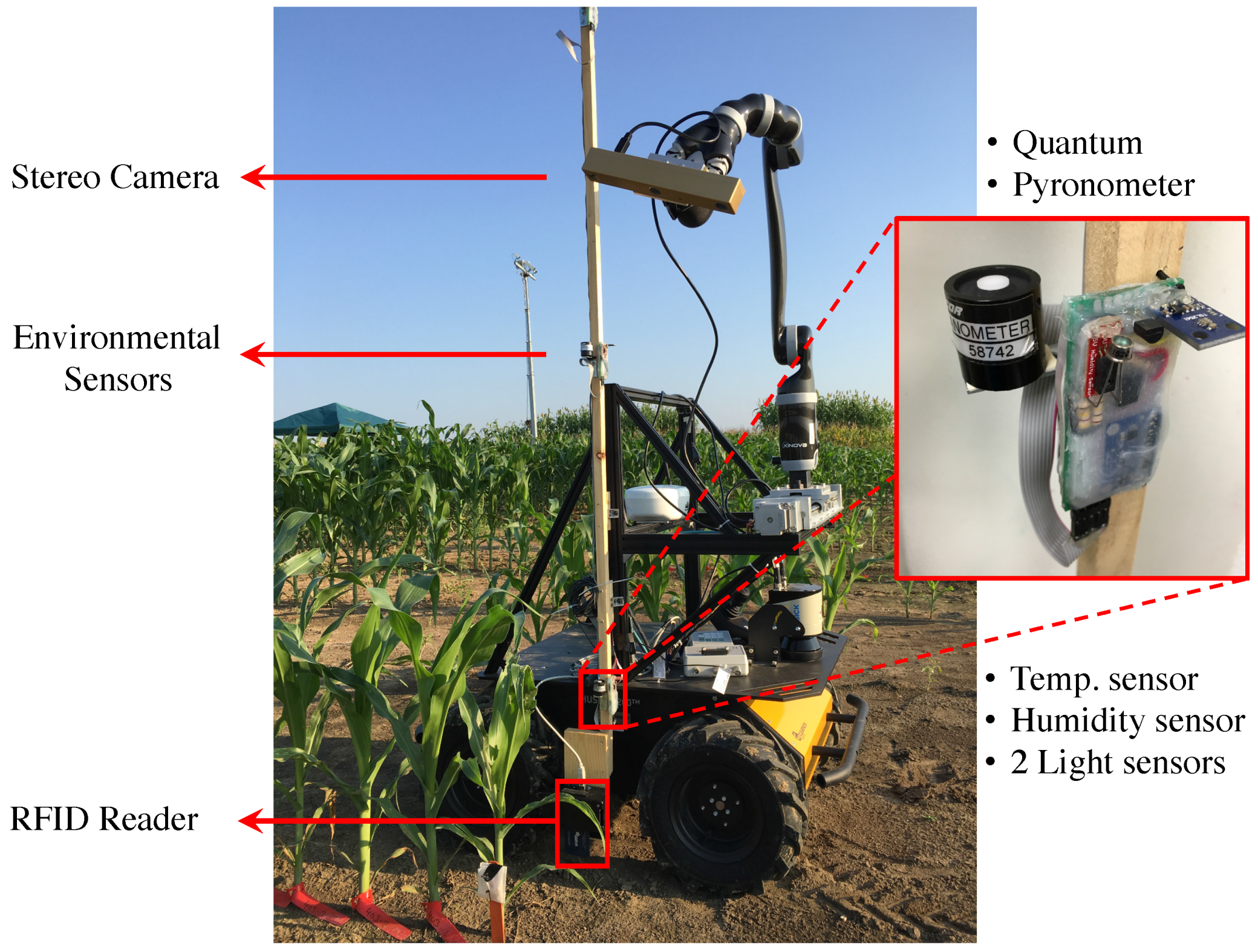
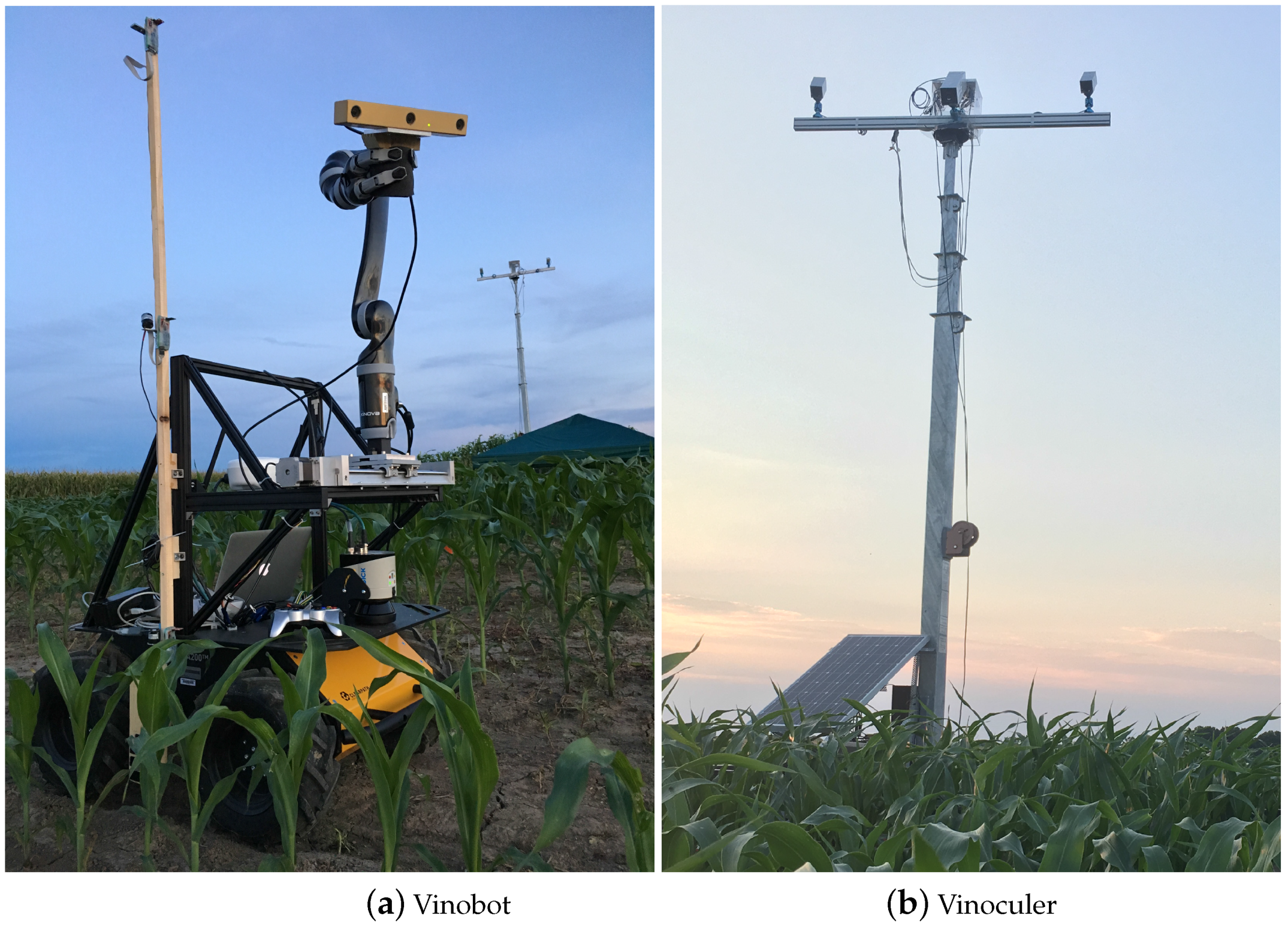
3.1.1. Vinobot
Hardware
Software
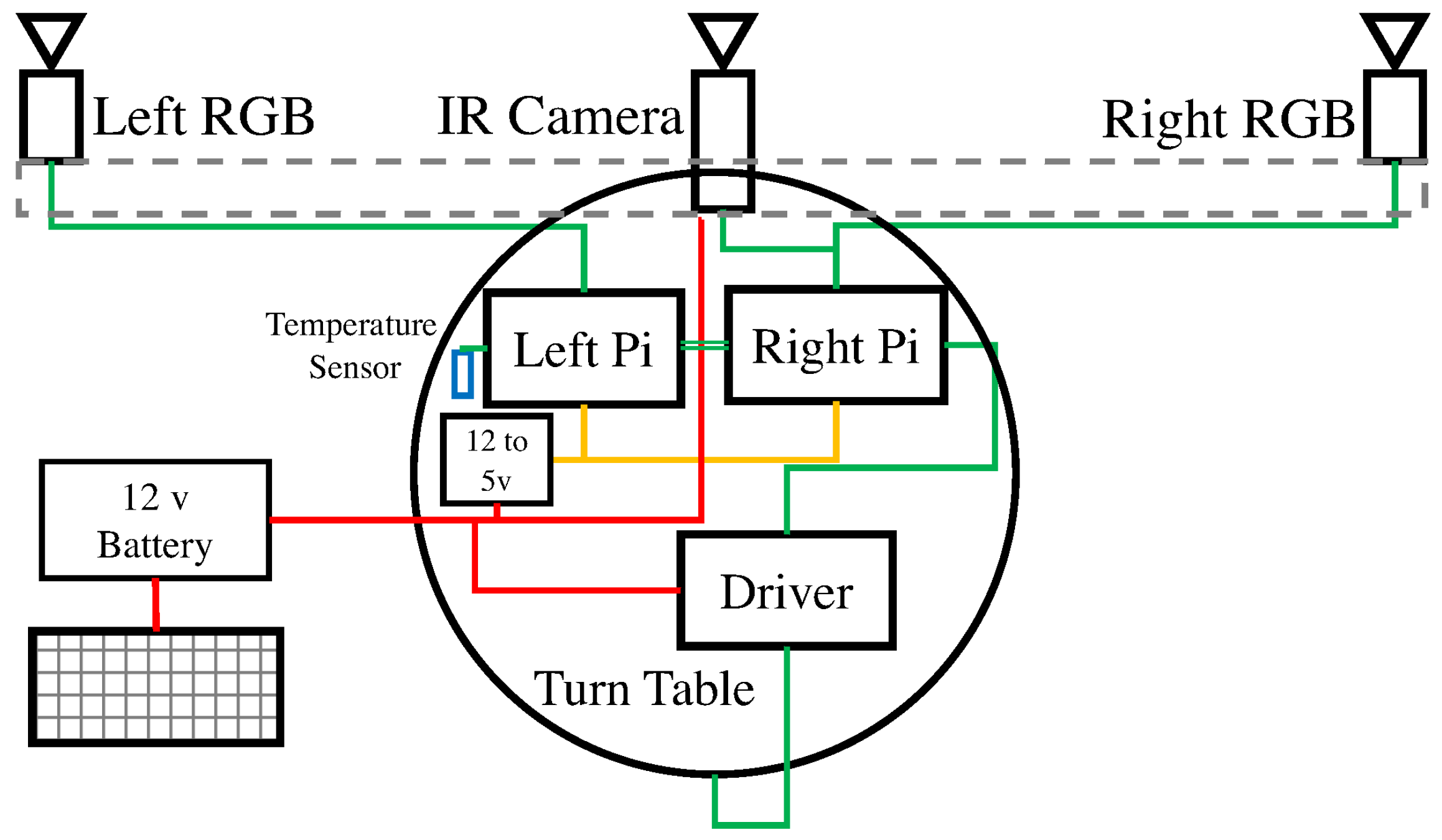
3.1.2. Vinoculer
Hardware
Software
3.2. Advantages over Other Systems
4. Experimental Results and Discussion
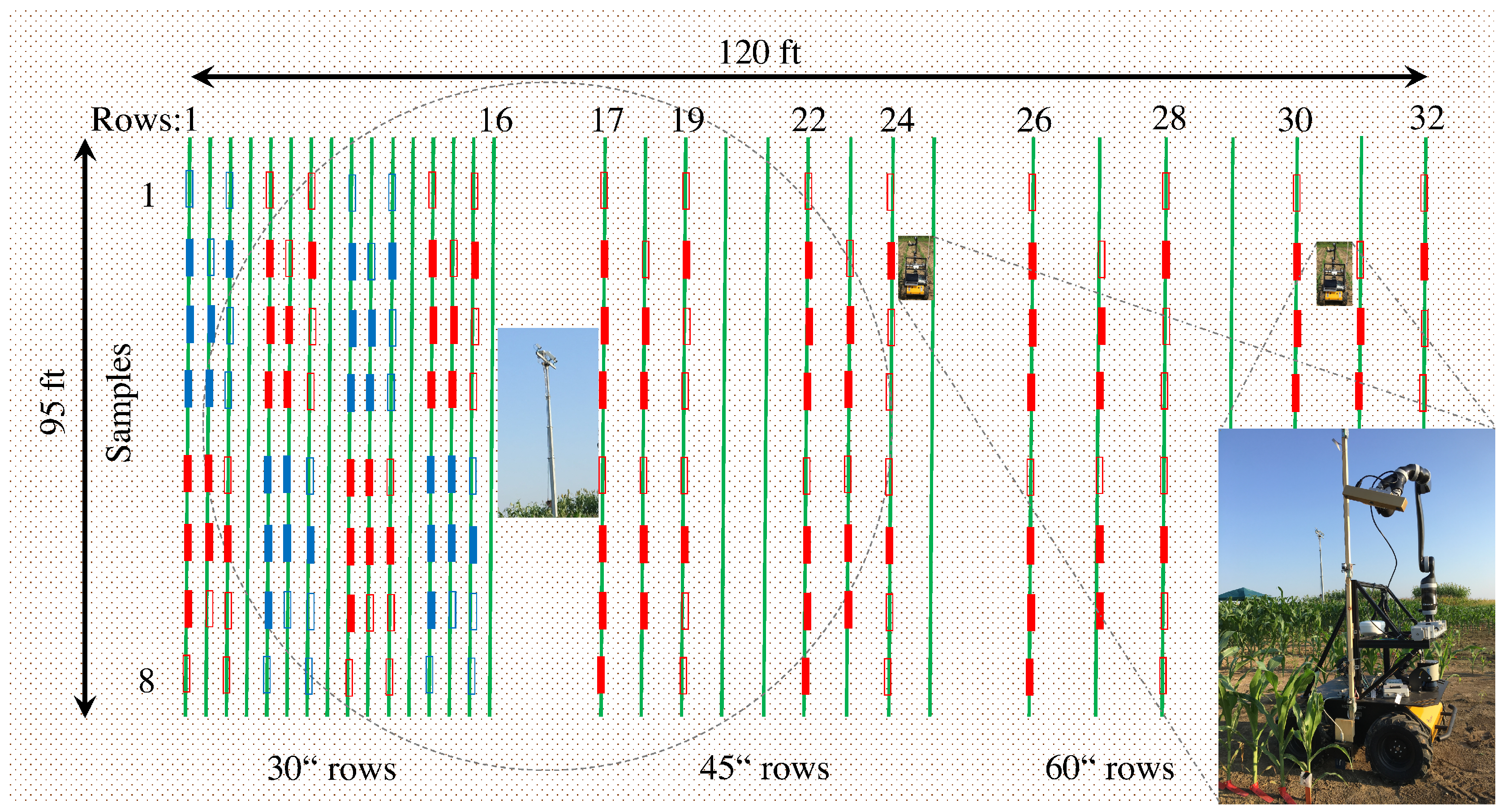
4.1. Vinobot
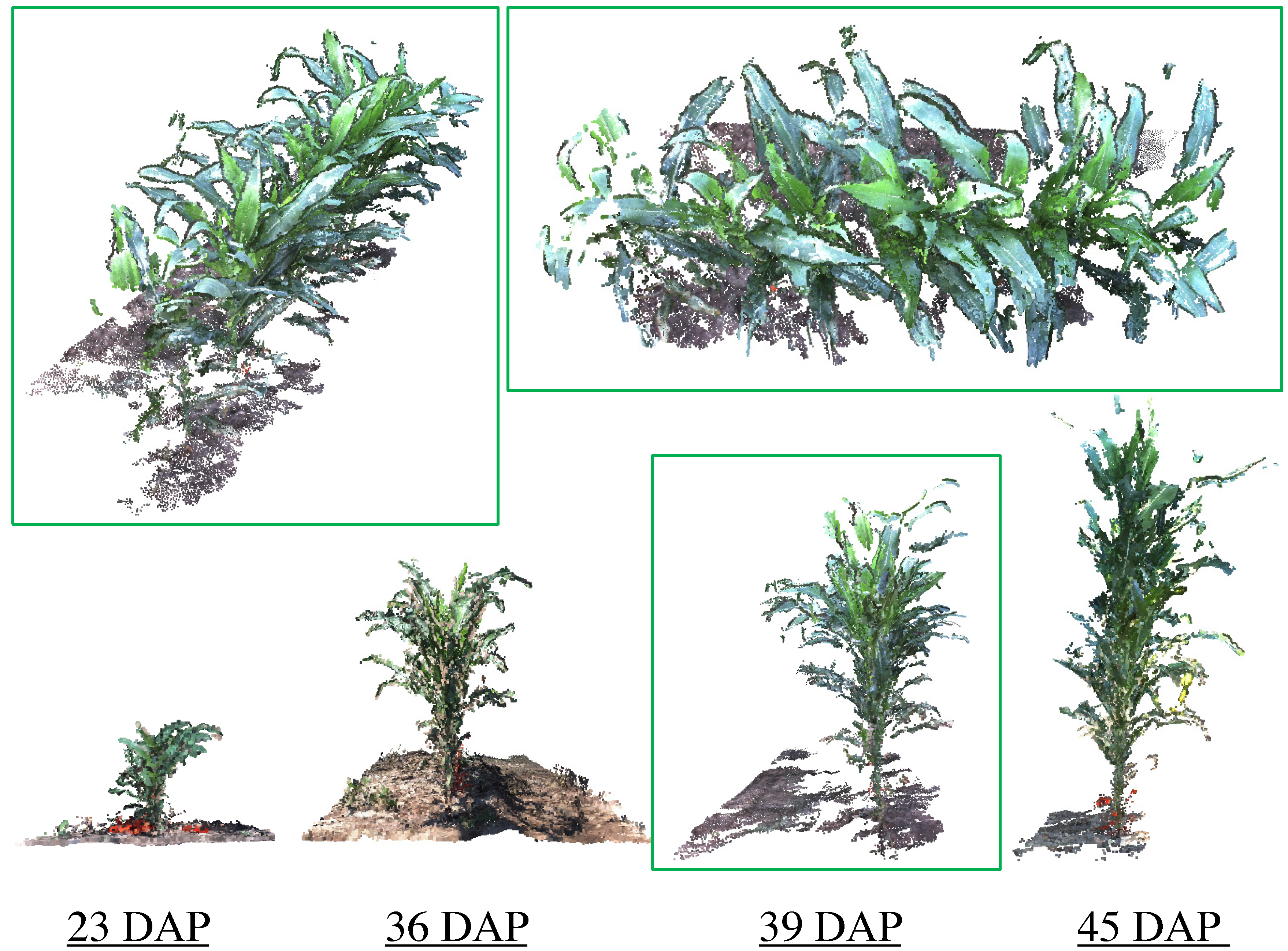
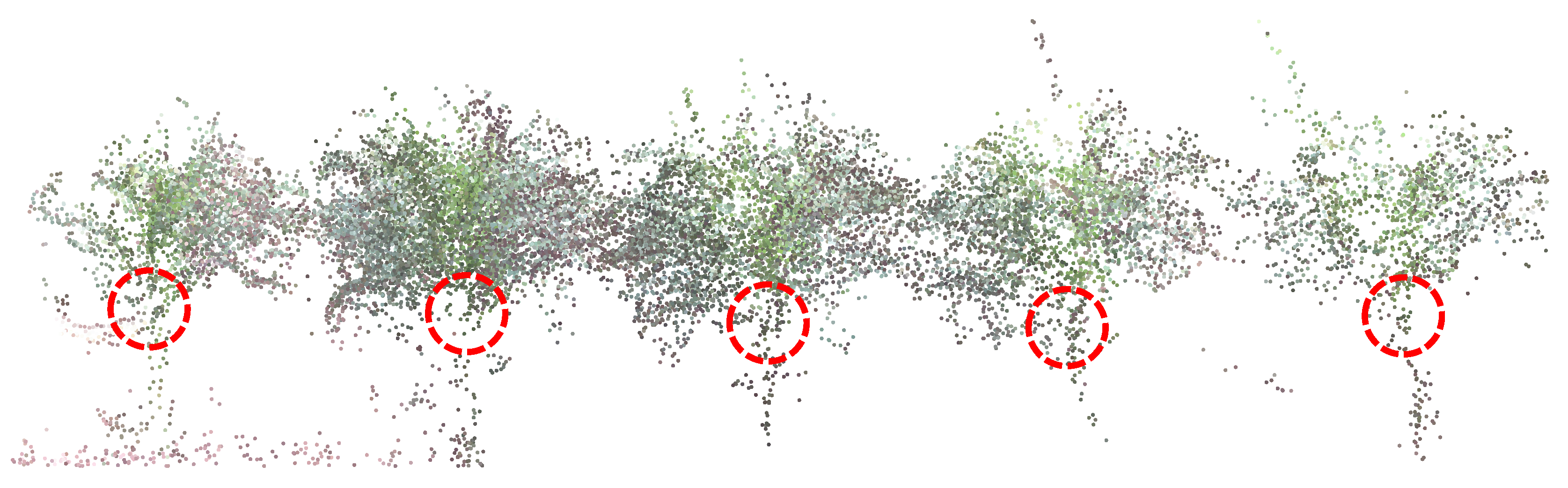
4.1.1. Traits from 3D Reconstruction
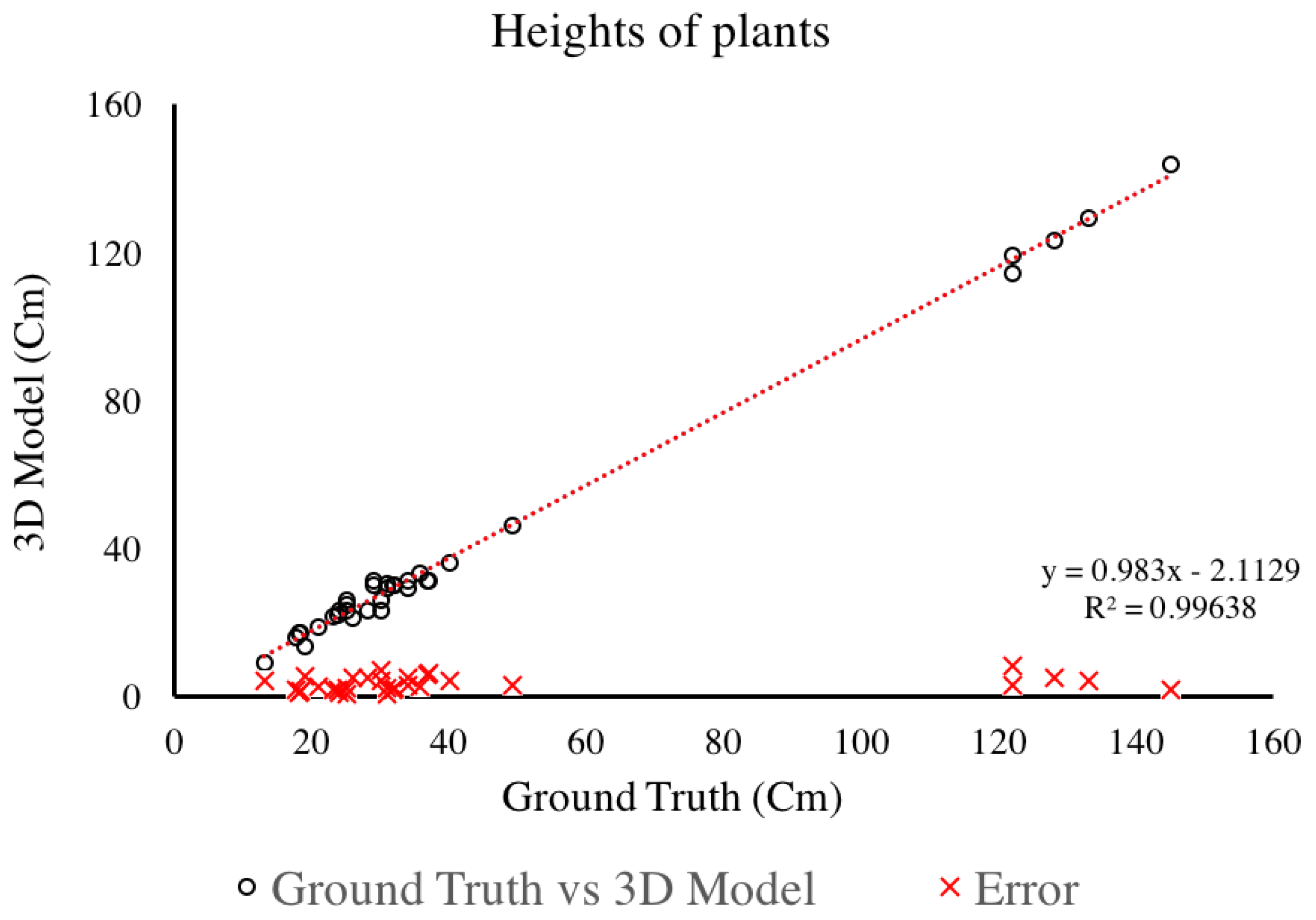
4.1.2. Plant Height
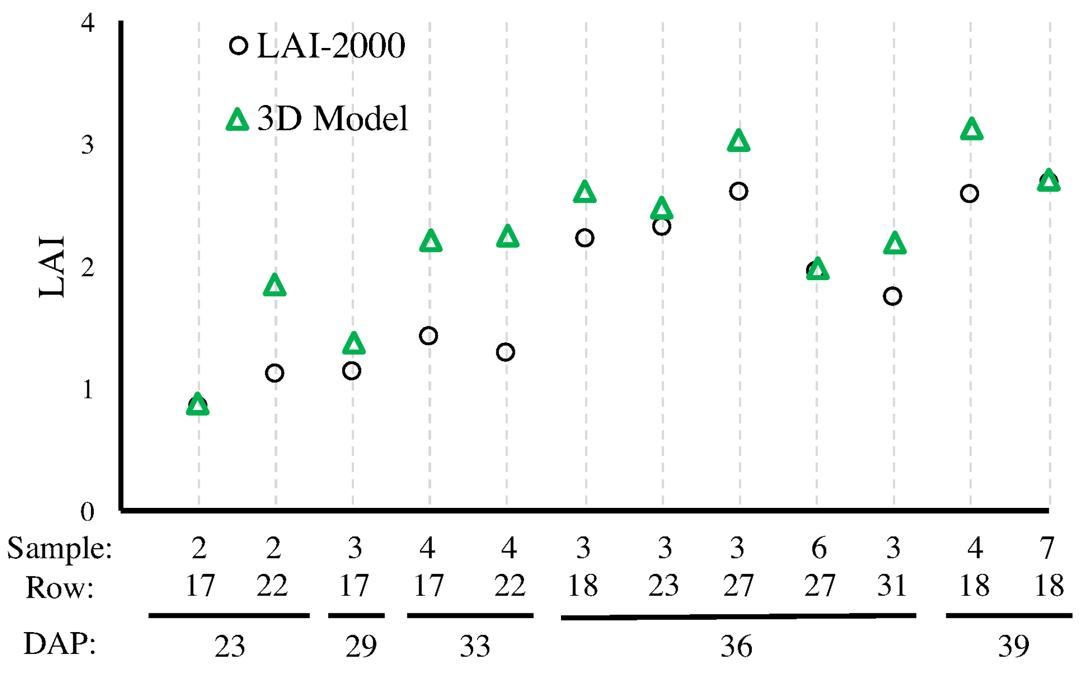
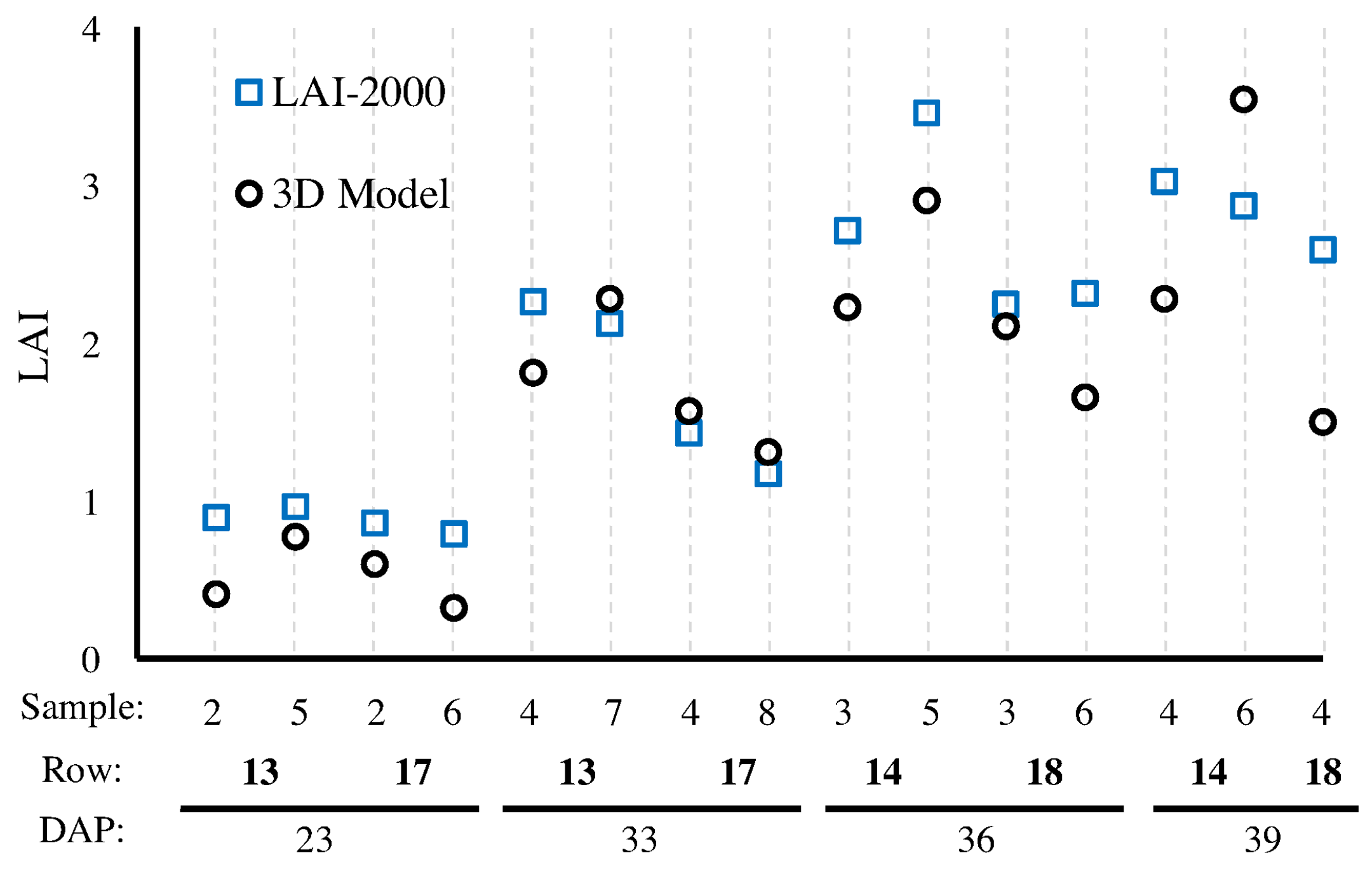
4.1.3. Leaf-Area Index
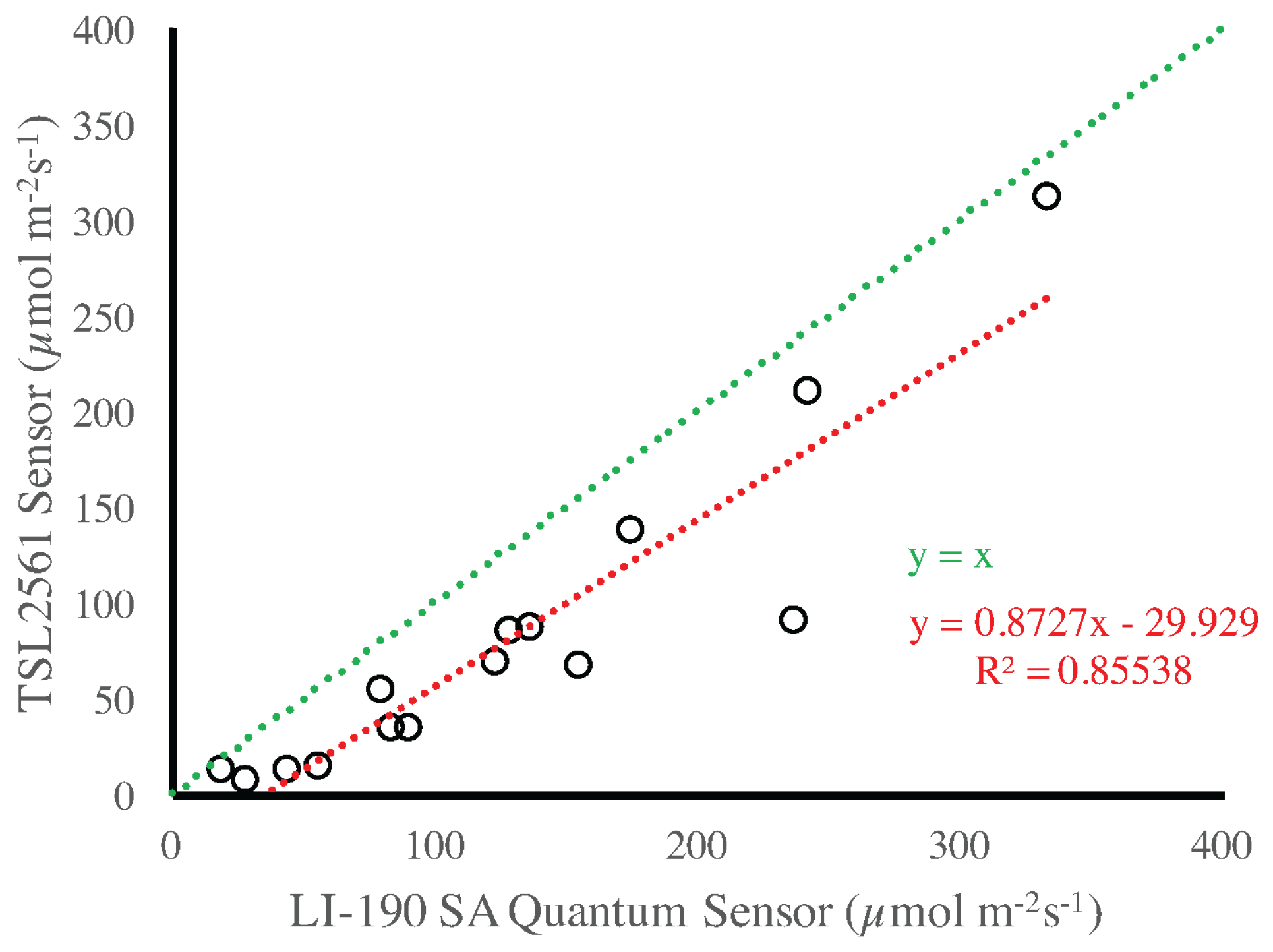
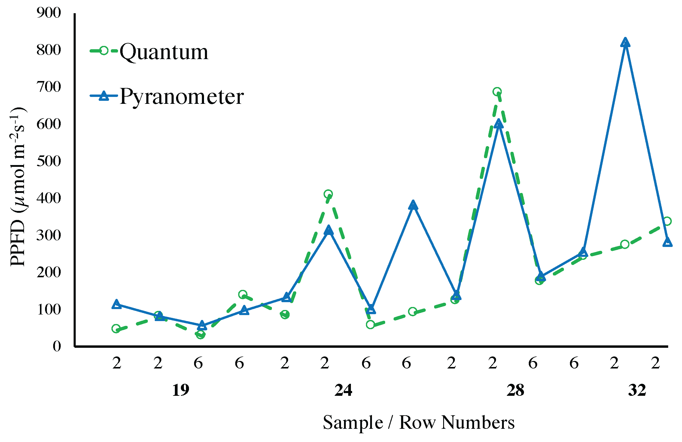
4.1.4. Light Exposure
4.2. Vinoculer
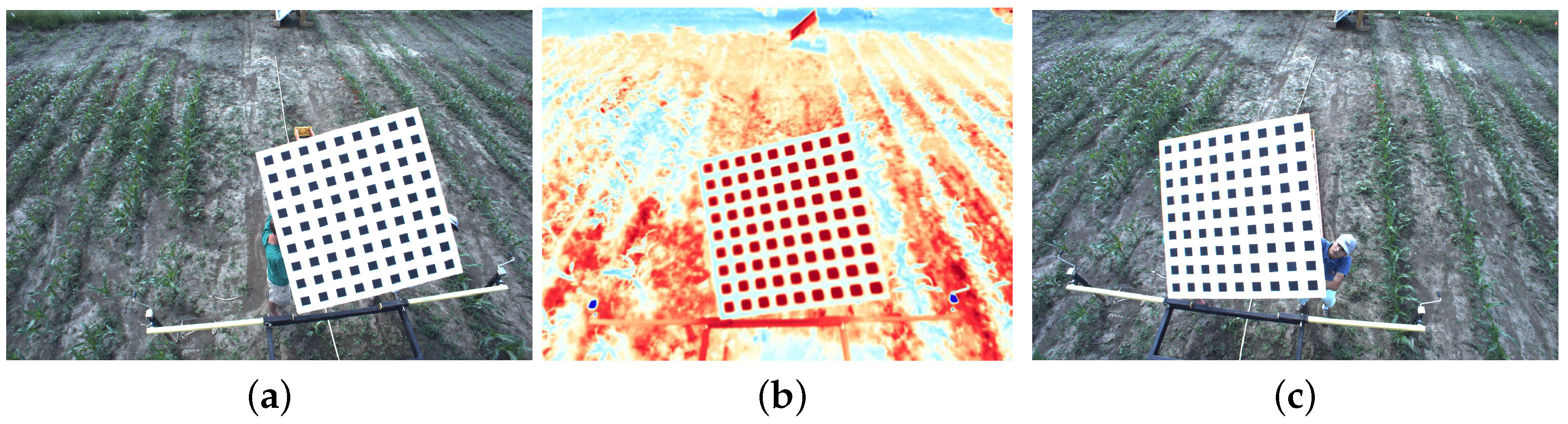
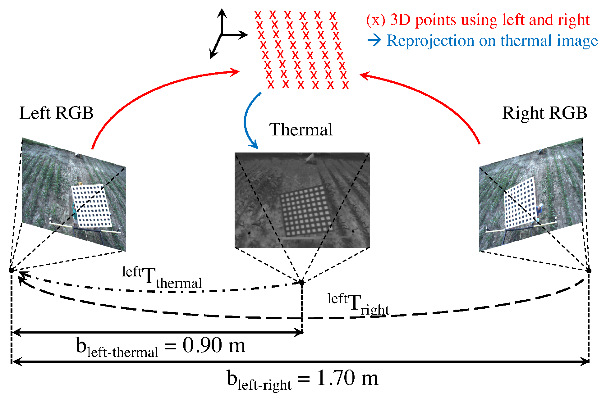
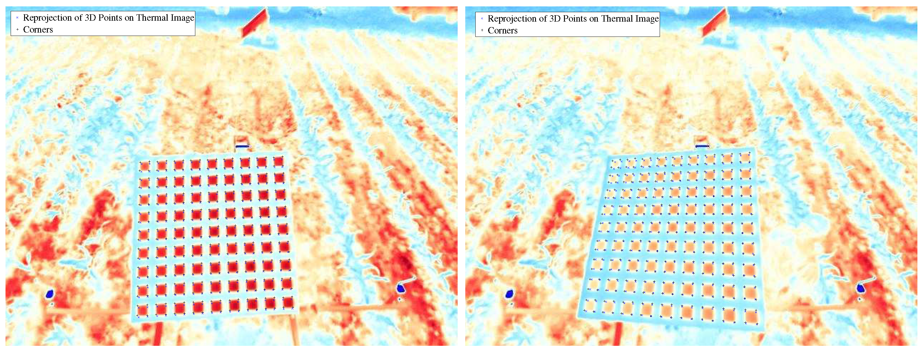
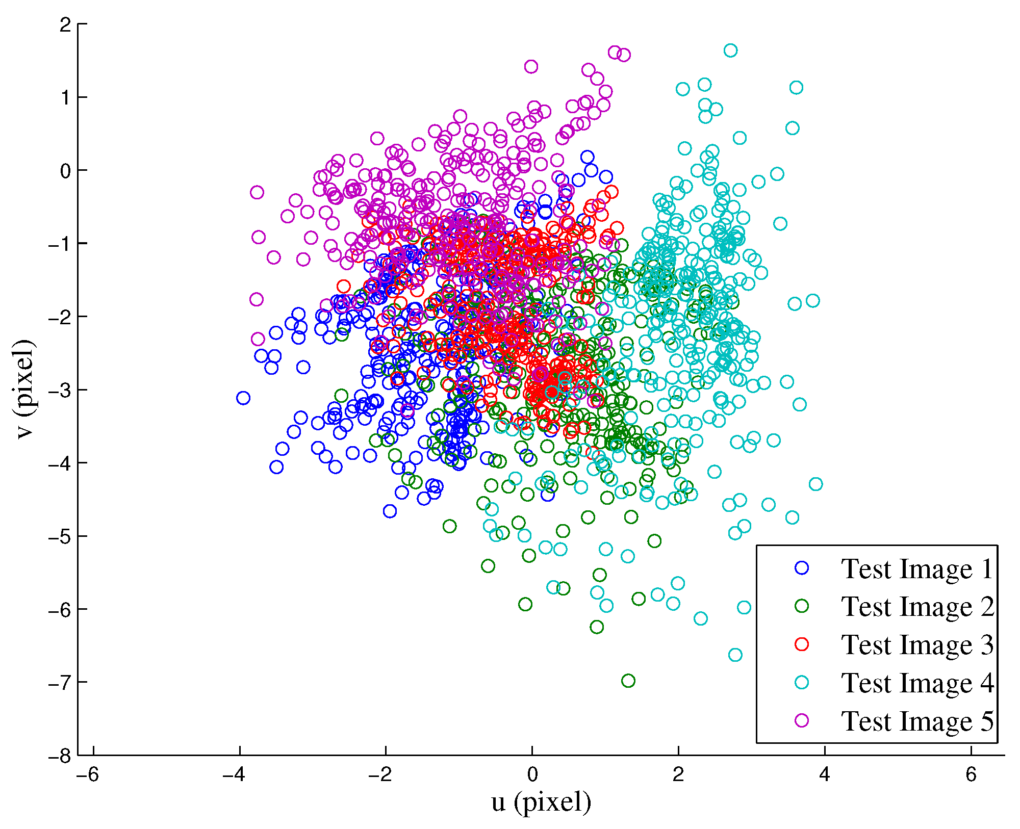
4.2.1. RGB to IR Camera Calibration
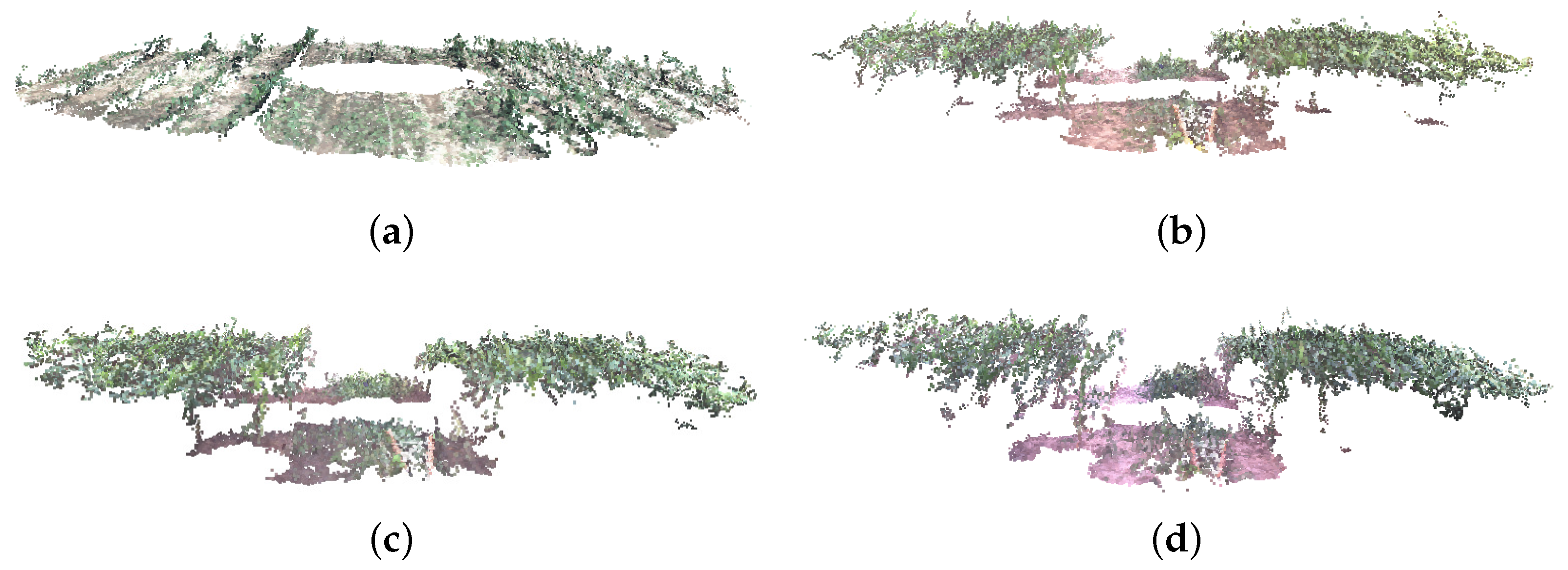
4.2.2. Traits from 3D Reconstruction
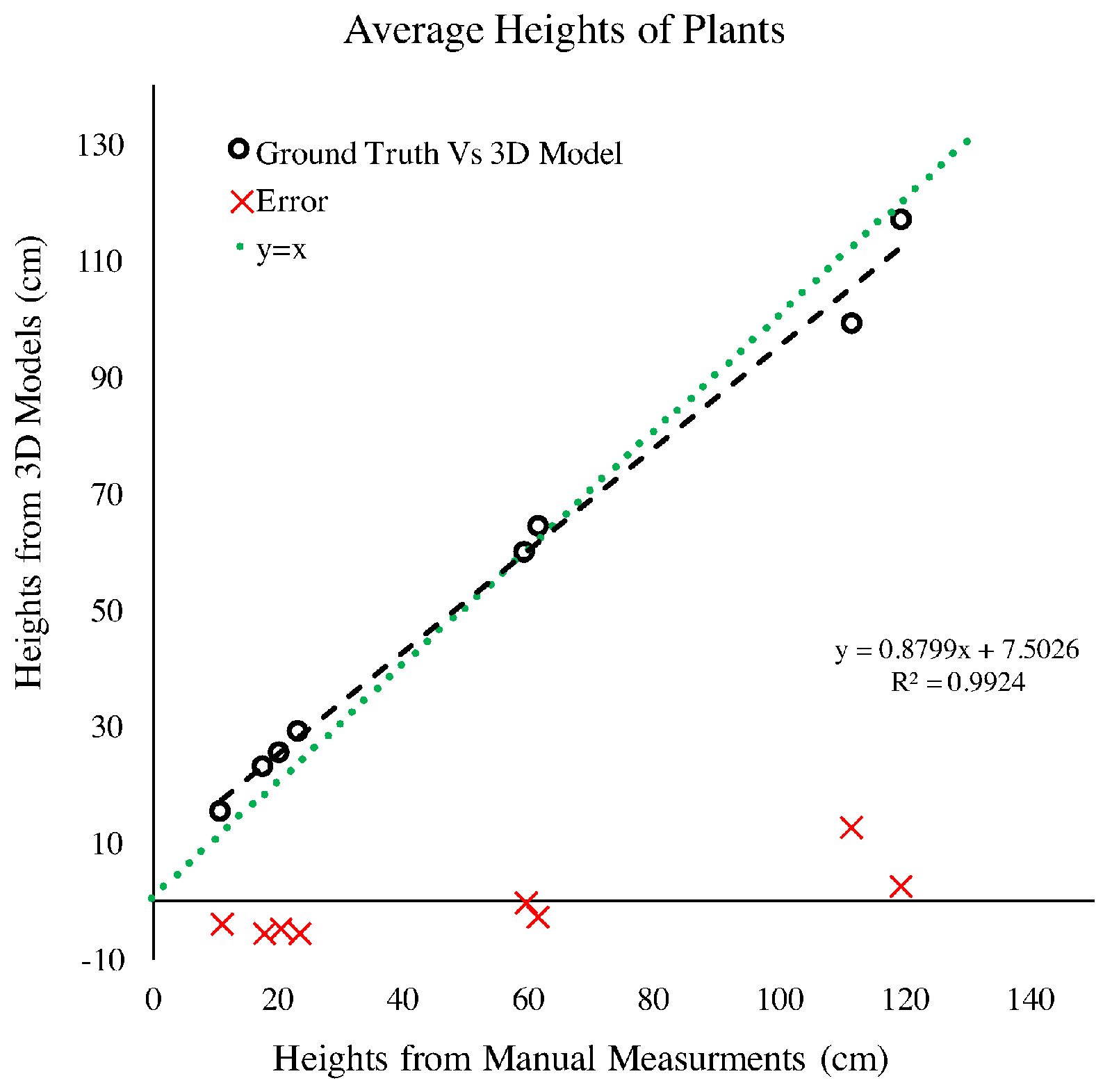
4.2.3. Plant Height
4.2.4. LAI Estimation
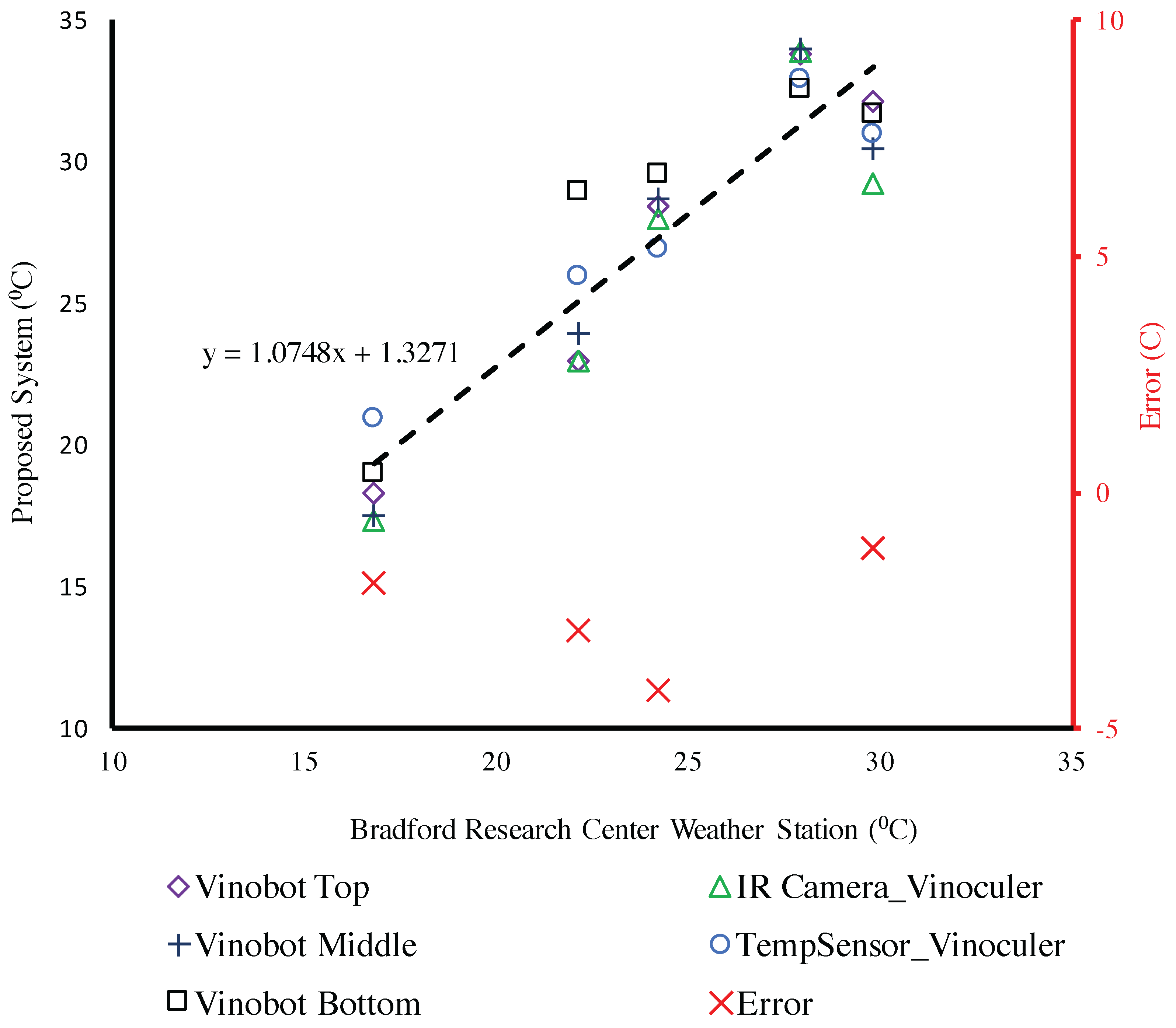
4.3. Environmental Data
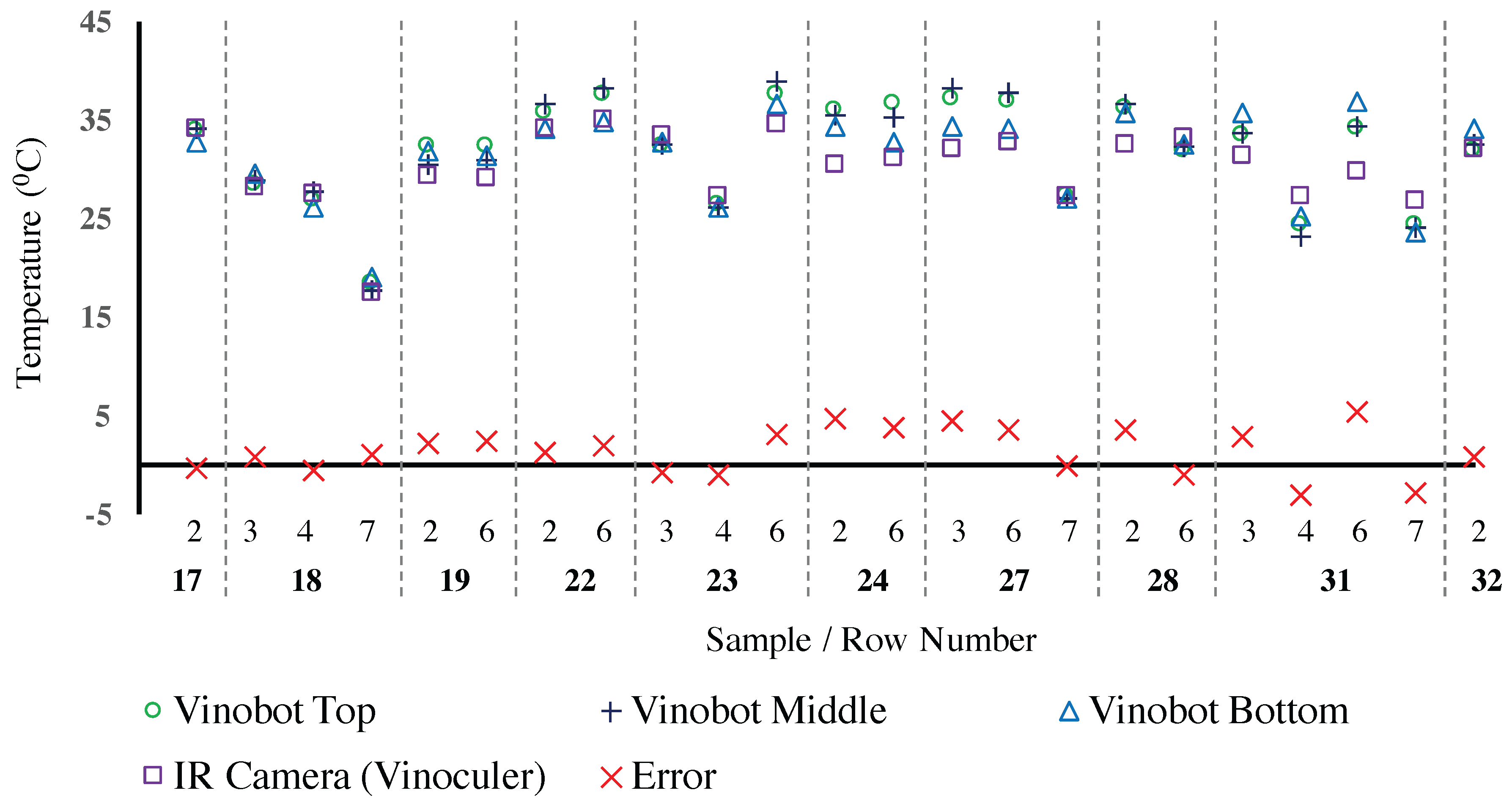
Temperature
5. Conclusions and Future Work
Acknowledgments
Author Contributions
Conflicts of Interest
References
- Fischer, G. World food and agriculture to 2030/50. In Proceedings of the Technical paper from the Expert Meeting on How to Feed the World in 2050, Rome, Italy, 24–26 June 2009; Volume 2050, pp. 24–26.
- Chaves, M.M.; Maroco, J.P.; Pereira, J.S. Understanding plant responses to drought—From genes to the whole plant. Funct. Plant Biol. 2003, 30, 239–264. [Google Scholar] [CrossRef]
- Araus, J.L.; Cairns, J.E. Field high-throughput phenotyping: The new crop breeding frontier. Trends Plant Sci. 2014, 19, 52–61. [Google Scholar] [CrossRef] [PubMed]
- Fiorani, F.; Schurr, U. Future scenarios for plant phenotyping. Annu. Rev. Plant Biol. 2013, 64, 267–291. [Google Scholar] [CrossRef] [PubMed]
- Sankaran, S.; Khot, L.R.; Espinoza, C.Z.; Jarolmasjed, S.; Sathuvalli, V.R.; Vandemark, G.J.; Miklas, P.N.; Carter, A.H.; Pumphrey, M.O.; Knowles, N.R.; et al. Low-altitude, high-resolution aerial imaging systems for row and field crop phenotyping: A review. Eur. J. Agron. 2015, 70, 112–123. [Google Scholar] [CrossRef]
- Shi, Y.; Thomasson, J.A.; Murray, S.C.; Pugh, N.A.; Rooney, W.L.; Shafian, S.; Rajan, N.; Rouze, G.; Morgan, C.L.; Neely, H.L.; et al. Unmanned Aerial Vehicles for High-Throughput Phenotyping and Agronomic Research. PLoS ONE 2016, 11, e0159781. [Google Scholar] [CrossRef] [PubMed]
- Field-Base HTTP Platform, Scnalyzer Field. Available online: http://www.lemnatec.com/products/hardware-solutions/scanalyzer-field (accessed on 22 January 2017).
- Kicherer, A.; Herzog, K.; Pflanz, M.; Wieland, M.; Rüger, P.; Kecke, S.; Kuhlmann, H.; Töpfer, R. An automated field phenotyping pipeline for application in grapevine research. Sensors 2015, 15, 4823–4836. [Google Scholar] [CrossRef] [PubMed]
- Virlet, N.; Sabermanesh, K.; Sadeghi-Tehran, P.; Hawkesford, M.J. Field Scanalyzer: An automated robotic field phenotyping platform for detailed crop monitoring. Funct. Plant Biol. 2017, 44, 143–153. [Google Scholar] [CrossRef]
- Morgan, K. A step towards an automatic tractor. Farm. Mech. 1958, 10, 440–441. [Google Scholar]
- Ruckelshausen, A.; Biber, P.; Dorna, M.; Gremmes, H.; Klose, R.; Linz, A.; Rahe, F.; Resch, R.; Thiel, M.; Trautz, D.; et al. BoniRob—An autonomous field robot platform for individual plant phenotyping. Precis. Agric. 2009, 9, 1. [Google Scholar]
- Hiremath, S.A.; van der Heijden, G.W.; van Evert, F.K.; Stein, A.; Ter Braak, C.J. Laser range finder model for autonomous navigation of a robot in a maize field using a particle filter. Comput. Electron. Agric. 2014, 100, 41–50. [Google Scholar] [CrossRef]
- Tisne, S.; Serrand, Y.; Bach, L.; Gilbault, E.; Ben Ameur, R.; Balasse, H.; Voisin, R.; Bouchez, D.; Durand-Tardif, M.; Guerche, P.; et al. Phenoscope: An automated large-scale phenotyping platform offering high spatial homogeneity. Plant J. 2013, 74, 534–544. [Google Scholar] [CrossRef] [PubMed]
- Andrade-Sanchez, P.; Gore, M.A.; Heun, J.T.; Thorp, K.R.; Carmo-Silva, A.E.; French, A.N.; Salvucci, M.E.; White, J.W. Development and evaluation of a field-based high-throughput phenotyping platform. Funct. Plant Biol. 2014, 41, 68–79. [Google Scholar] [CrossRef]
- Barker, J.; Zhang, N.; Sharon, J.; Steeves, R.; Wang, X.; Wei, Y.; Poland, J. Development of a field-based high-throughput mobile phenotyping platform. Comput. Electron. Agric. 2016, 122, 74–85. [Google Scholar] [CrossRef]
- Chen, C.Y.; Butts, C.L.; Dang, P.M.; Wang, M.L. Advances in Phenotyping of Functional Traits. In Phenomics in Crop Plants: Trends, Options and Limitations; Springer: Berlin/Heidelberg, Germany, 2015; pp. 163–180. [Google Scholar]
- Basu, P.S.; Srivastava, M.; Singh, P.; Porwal, P.; Kant, R.; Singh, J. High-precision phenotyping under controlled versus natural environments. In Phenomics in Crop Plants: Trends, Options and Limitations; Springer: Berlin/Heidelberg, Germany, 2015; pp. 27–40. [Google Scholar]
- Von Mogel, K.H. Phenomics Revolution. CSA News 2013. [Google Scholar] [CrossRef]
- Araus, J.L.; Slafer, G.A.; Royo, C.; Serret, M.D. Breeding for yield potential and stress adaptation in cereals. Crit. Rev. Plant Sci. 2008, 27, 377–412. [Google Scholar] [CrossRef]
- Busemeyer, L.; Mentrup, D.; Möller, K.; Wunder, E.; Alheit, K.; Hahn, V.; Maurer, H.P.; Reif, J.C.; Würschum, T.; Müller, J.; et al. Breedvision–A multi-sensor platform for non-destructive field-based phenotyping in plant breeding. Sensors 2013, 13, 2830–2847. [Google Scholar] [CrossRef] [PubMed]
- Åstrand, B.; Baerveldt, A.J. A vision based row-following system for agricultural field machinery. Mechatronics 2005, 15, 251–269. [Google Scholar] [CrossRef]
- Deery, D.; Jimenez-Berni, J.; Jones, H.; Sirault, X.; Furbank, R. Proximal remote sensing buggies and potential applications for field-based phenotyping. Agronomy 2014, 4, 349–379. [Google Scholar] [CrossRef]
- Hamza, M.; Anderson, W. Soil compaction in cropping systems: A review of the nature, causes and possible solutions. Soil Till. Res. 2005, 82, 121–145. [Google Scholar] [CrossRef]
- Costa, F.G.; Ueyama, J.; Braun, T.; Pessin, G.; Osório, F.S.; Vargas, P.A. The use of unmanned aerial vehicles and wireless sensor network in agricultural applications. In Proceedings of the 2012 IEEE International Geoscience and Remote Sensing Symposium (IGARSS), Munich, Germany, 22–27 July 2012; pp. 5045–5048.
- Sugiura, R.; Noguchi, N.; Ishii, K. Remote-sensing technology for vegetation monitoring using an unmanned helicopter. Biosyst. Eng. 2005, 90, 369–379. [Google Scholar] [CrossRef]
- Swain, K.C.; Thomson, S.J.; Jayasuriya, H.P. Adoption of an unmanned helicopter for low-altitude remote sensing to estimate yield and total biomass of a rice crop. Trans. ASABE 2010, 53, 21–27. [Google Scholar] [CrossRef]
- Göktoğan, A.H.; Sukkarieh, S.; Bryson, M.; Randle, J.; Lupton, T.; Hung, C. A rotary-wing unmanned air vehicle for aquatic weed surveillance and management. In Proceedings of the 2nd International Symposium on UAVs, Reno, NV, USA, 8–10 June 2009; Springer: Berlin/Heidelberg, Germany, 2009; pp. 467–484. [Google Scholar]
- Department of Transportation, Federal Aviation Administration. Operation and Certification of Small Unmanned Aircraft Systems; Final Rule; Rules and Regulations 14 CFR Parts 21, 43, 61, et al.; Department of Transportation, Federal Aviation Administration: Washington, DC, USA, 2016; Volume 81.
- Mulligan, J. Legal and Policy Issues in the FAA Modernization and Reform Act of 2012. Issues Aviat. Law Policy 2011, 11, 395. [Google Scholar]
- DeSouza, G.N.; Kak, A.C. Vision for Mobile Robot Navigation: A Survey. IEEE Trans. Pattern Anal. Mach. Intell. 2002, 24, 237–267. [Google Scholar] [CrossRef]
- Søgaard, H.T.; Olsen, H.J. Determination of crop rows by image analysis without segmentation. Comput. Electron. Agric. 2003, 38, 141–158. [Google Scholar] [CrossRef]
- Tillett, N.; Hague, T.; Miles, S. Inter-row vision guidance for mechanical weed control in sugar beet. Comput. Electron. Agric. 2002, 33, 163–177. [Google Scholar] [CrossRef]
- Shalal, N.; Low, T.; McCarthy, C.; Hancock, N. Orchard mapping and mobile robot localisation using on-board camera and laser scanner data fusion–Part A: Tree detection. Comput. Electron. Agric. 2015, 119, 254–266. [Google Scholar] [CrossRef]
- Shalal, N.; Low, T.; McCarthy, C.; Hancock, N. Orchard mapping and mobile robot localisation using on-board camera and laser scanner data fusion–Part B: Mapping and localisation. Comput. Electron. Agric. 2015, 119, 267–278. [Google Scholar] [CrossRef]
- English, A.; Ross, P.; Ball, D.; Corke, P. Vision based guidance for robot navigation in agriculture. In Proceedings of the 2014 IEEE International Conference on Robotics and Automation (ICRA), Hong Kong, China, 31 May–7 June 2014; pp. 1693–1698.
- Hiremath, S.; van Evert, F.; Heijden, V.D.G.; ter Braak, C.; Stein, A. Image-based particle filtering for robot navigation in a maize field. In Proceedings of the Workshop on Agricultural Robotics (IROS 2012), Vilamoura, Portugal, 7–12 October 2012.
- Yol, E.; Toker, C.; Uzun, B. Traits for Phenotyping. In Phenomics in Crop Plants: Trends, Options and Limitations; Springer: Berlin/Heidelberg, Germany, 2015; pp. 11–26. [Google Scholar]
- Fahlgren, N.; Gehan, M.A.; Baxter, I. Lights, camera, action: High-throughput plant phenotyping is ready for a close-up. Curr. Opin. Plant Biol. 2015, 24, 93–99. [Google Scholar] [CrossRef] [PubMed]
- Ruckelshausen, A.; Busemeyer, L. Toward Digital and Image-Based Phenotyping. In Phenomics in Crop Plants: Trends, Options and Limitations; Springer: Berlin/Heidelberg, Germany, 2015; pp. 41–60. [Google Scholar]
- Rousseau, D.; Dee, H.; Pridmore, T. Imaging Methods for Phenotyping of Plant Traits. In Phenomics in Crop Plants: Trends, Options and Limitations; Springer: Berlin/Heidelberg, Germany, 2015; pp. 61–74. [Google Scholar]
- McCarthy, C.L.; Hancock, N.H.; Raine, S.R. Applied machine vision of plants: a review with implications for field deployment in automated farming operations. Intell. Serv. Robot. 2010, 3, 209–217. [Google Scholar] [CrossRef] [Green Version]
- Scnalyzer 3D High Throughput. Available online: http://www.lemnatec.com/products/hardware-solutions/scanalyzer-3d-high-throughput (accessed on 22 January 2017).
- Topp, C.N.; Iyer-Pascuzzi, A.S.; Anderson, J.T.; Lee, C.R.; Zurek, P.R.; Symonova, O.; Zheng, Y.; Bucksch, A.; Mileyko, Y.; Galkovskyi, T.; et al. 3D phenotyping and quantitative trait locus mapping identify core regions of the rice genome controlling root architecture. Proc. Natl. Acad. Sci. USA 2013, 110, E1695–E1704. [Google Scholar] [CrossRef] [PubMed]
- Nakini, T.K.D.; DeSouza, G.N. Distortion Correction in 3D-Modeling of Root Systems for Plant Phenotyping. In Proceedings of the Computer Vision—ECCV 2014 Workshops, Zurich, Switzerland, 6–7 September 2014; Springer: Berlin/Heidelberg, Germany, 2014; pp. 140–157. [Google Scholar]
- Piñeros, M.A.; Larson, B.G.; Shaff, J.E.; Schneider, D.J.; Falcão, A.X.; Yuan, L.; Clark, R.T.; Craft, E.J.; Davis, T.W.; Pradier, P.L.; et al. Evolving technologies for growing, imaging and analyzing 3D root system architecture of crop plants. J. Integr. Plant Biol. 2016, 58, 230–241. [Google Scholar] [CrossRef] [PubMed]
- Jay, S.; Rabatel, G.; Hadoux, X.; Moura, D.; Gorretta, N. In-field crop row phenotyping from 3D modeling performed using Structure from Motion. Comput. Electron. Agric. 2015, 110, 70–77. [Google Scholar] [CrossRef]
- Pierrot-Deseilligny, M. Micmac Documentation: MicMac, Apero, Pastis and Other Beverages in A Nutshell. Available online: http://logiciels.ign.fr (accessed on 24 July 2014).
- Gregersen, P.L.; Culetic, A.; Boschian, L.; Krupinska, K. Plant senescence and crop productivity. Plant Mol. Biol. 2013, 82, 603–622. [Google Scholar] [CrossRef] [PubMed]
- Chapman, S.C.; Merz, T.; Chan, A.; Jackway, P.; Hrabar, S.; Dreccer, M.F.; Holland, E.; Zheng, B.; Ling, T.J.; Jimenez-Berni, J. Pheno-copter: A low-altitude, autonomous remote-sensing robotic helicopter for high-throughput field-based phenotyping. Agronomy 2014, 4, 279–301. [Google Scholar] [CrossRef]
- Cruzan, M.B.; Weinstein, B.G.; Grasty, M.R.; Kohrn, B.F.; Hendrickson, E.C.; Arredondo, T.M.; Thompson, P.G. Small Unmanned Aerial Vehicles (Micro-UAVs, Drones) in Plant Ecology. Appl. Plant Sci. 2016, 4, 1600041. [Google Scholar] [CrossRef] [PubMed]
- Anthony, D.; Elbaum, S.; Lorenz, A.; Detweiler, C. On crop height estimation with UAVs. In Proceedings of the 2014 IEEE/RSJ International Conference on Intelligent Robots and Systems (IROS 2014), Chicago, IL, USA, 14–18 September 2014; pp. 4805–4812.
- Quigley, M.; Conley, K.; Gerkey, B.; Faust, J.; Foote, T.; Leibs, J.; Wheeler, R.; Ng, A.Y. ROS: An Open-Source Robot Operating System; ICRA Workshop on Open Source Software: Kobe, Japan, 2009; Volume 3, p. 5. [Google Scholar]
- Shafiekhani, A.; DeSouza, G. Vinobot and Vinoculer Data (Sample). Available online: https://missouriepscor.org/data/vinobot-and-vinoculer-data-sample (accessed on 26 September 2016).
- Wu, C. VisualSFM: A Visual Structure from Motion System. 2011. Available online: http://www.cs.washington.edu/homes/ccwu/vsfm/ (accessed on 22 January 2017).
- Bréda, N.J. Ground-based measurements of leaf area index: A review of methods, instruments and current controversies. J. Exp. Bot. 2003, 54, 2403–2417. [Google Scholar] [CrossRef] [PubMed]
- Chen, J.M.; Pavlic, G.; Brown, L.; Cihlar, J.; Leblanc, S.; White, H.; Hall, R.; Peddle, D.; King, D.; Trofymow, J.; et al. Derivation and validation of Canada-wide coarse-resolution leaf area index maps using high-resolution satellite imagery and ground measurements. Remote Sens. Environ. 2002, 80, 165–184. [Google Scholar] [CrossRef]
- Pokornỳ, R.; Marek, M. Test of accuracy of LAI estimation by LAI-2000 under artificially changed leaf to wood area proportions. Biol. Plant. 2000, 43, 537–544. [Google Scholar] [CrossRef]
- Stenberg, P.; Linder, S.; Smolander, H.; Flower-Ellis, J. Performance of the LAI-2000 plant canopy analyzer in estimating leaf area index of some Scots pine stands. Tree Physiol. 1994, 14, 981–995. [Google Scholar] [CrossRef] [PubMed]
- Instruments, A. Conversions-PPF to Lux; Apogee Instruments, Inc.: Logan, UT, USA. Available online: http://www.apogeeinstruments.com/conversion-ppf-to-lux/ (accessed on 22 January 2017).
- Zhang, Z. A flexible new technique for camera calibration. IEEE Trans. Pattern Anal. Mach. Intell. 2000, 22, 1330–1334. [Google Scholar] [CrossRef]
- Bouguet, J.Y. Camera Calibration Toolbox for Matlab. 2004. Available online: http://www.vision.caltech.edu/bouguetj/calib_doc (accessed on 22 January 2017).
- Goudriaan, J. The bare bones of leaf-angle distribution in radiation models for canopy photosynthesis and energy exchange. Agric. For. Meteorol. 1988, 43, 155–169. [Google Scholar] [CrossRef]
- AgEBB. Bradford Weather Station. Available online: http://agebb.missouri.edu/weather/realtime/columbiaBREC.asp (accessed on 22 January 2017).


| Platform | Cost (US$) |
|---|---|
| Vinoculer | 5 K |
| UAV | 16–80 K |
| Platform | Payload | Flight Time | Area/Flight | Availability | Total Area Covered | Type of Camera | Max Wind Speed |
|---|---|---|---|---|---|---|---|
| Phenocopter [49] | 1.5 kg | 30 min | 3 ha | 7 flights/day | 21 ha/day | RGB, Thermal and NIR | 11 m/s |
| Vinoculer | 20 kg | - | - | 24/7 | 2.2 ha/day | Limited by payload | 22.3 m/s 1 |
| Platforms | Type | Plants/h | ha/h | Images/h | Bytes/h | Main Capabilities |
|---|---|---|---|---|---|---|
| Vinobot | Semi-automated | 35,430 | 0.41 | 324,000 | 380 G | RGB, temperature, humidity, and light intensity |
| Vinoculer | Fully-automated | 12,648 | 0.09 | 2592 | 5.4 G | Mobile, 24/7, Stereo RGB and IR imaging, Air Temperature |
| “Phenomobile” [14] | Manually-driven | - | 0.84 | - | 2.094 M | IR, multi-spectral imaging, and sonar sensors |
| [9] | Fully-automated | - | 0.002 | 115 | 6.7 G | Confined, 24/7, RGB, Multispectral, Fluorescence intensity imaging |
| Platforms | Type | Plants/h | Images/h |
|---|---|---|---|
| Vinobot | Outdoor/Semi-automated | 120 | 1440 |
| [16] | Indoor/Fully-automated | 25 | 375 |
| Phenoscope [13] | Indoor/Fully-automated | 185 | 3750 |
| Plot Type vs. Sampling Method | Manually | Vinoculer | Vinobot |
|---|---|---|---|
| 30″ (76 cm) Rows | √ | √ | |
| 45″ (114 cm) Rows | √ | √ | √ |
| 60″ (152 cm) Rows | √ | √ |
© 2017 by the authors; licensee MDPI, Basel, Switzerland. This article is an open access article distributed under the terms and conditions of the Creative Commons Attribution (CC BY) license (http://creativecommons.org/licenses/by/4.0/).
Share and Cite
Shafiekhani, A.; Kadam, S.; Fritschi, F.B.; DeSouza, G.N. Vinobot and Vinoculer: Two Robotic Platforms for High-Throughput Field Phenotyping. Sensors 2017, 17, 214. https://doi.org/10.3390/s17010214
Shafiekhani A, Kadam S, Fritschi FB, DeSouza GN. Vinobot and Vinoculer: Two Robotic Platforms for High-Throughput Field Phenotyping. Sensors. 2017; 17(1):214. https://doi.org/10.3390/s17010214
Chicago/Turabian StyleShafiekhani, Ali, Suhas Kadam, Felix B. Fritschi, and Guilherme N. DeSouza. 2017. "Vinobot and Vinoculer: Two Robotic Platforms for High-Throughput Field Phenotyping" Sensors 17, no. 1: 214. https://doi.org/10.3390/s17010214