
Measurement and Geometric Modelling of Human Spine Posture for Medical Rehabilitation Purposes Using a Wearable Monitoring System Based on Inertial Sensors


Abstract
:1. Introduction
2. Materials and Methods
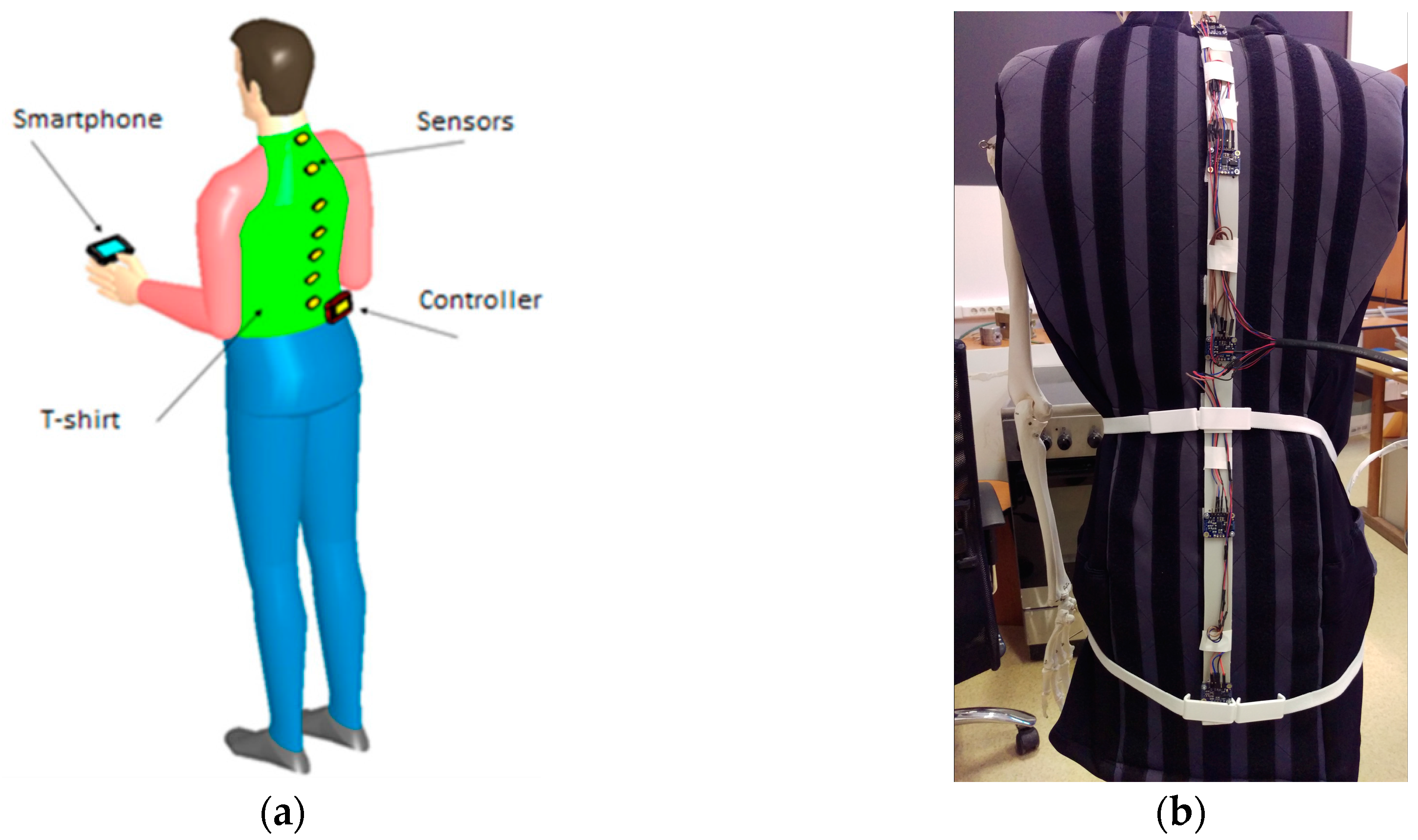
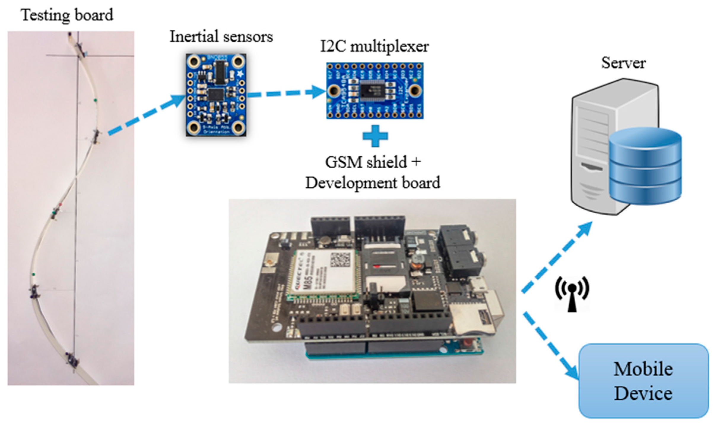
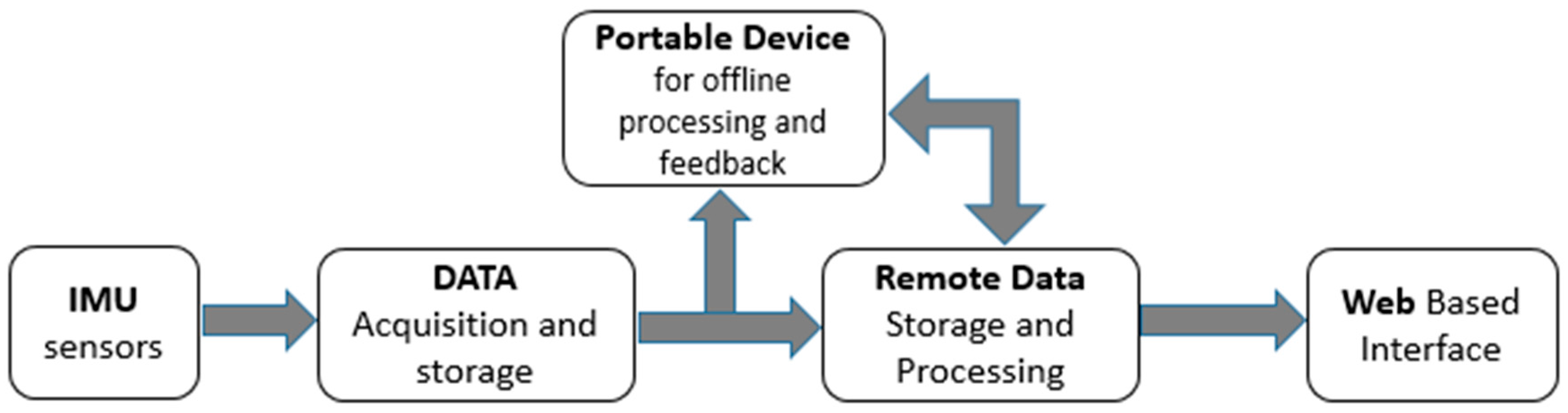
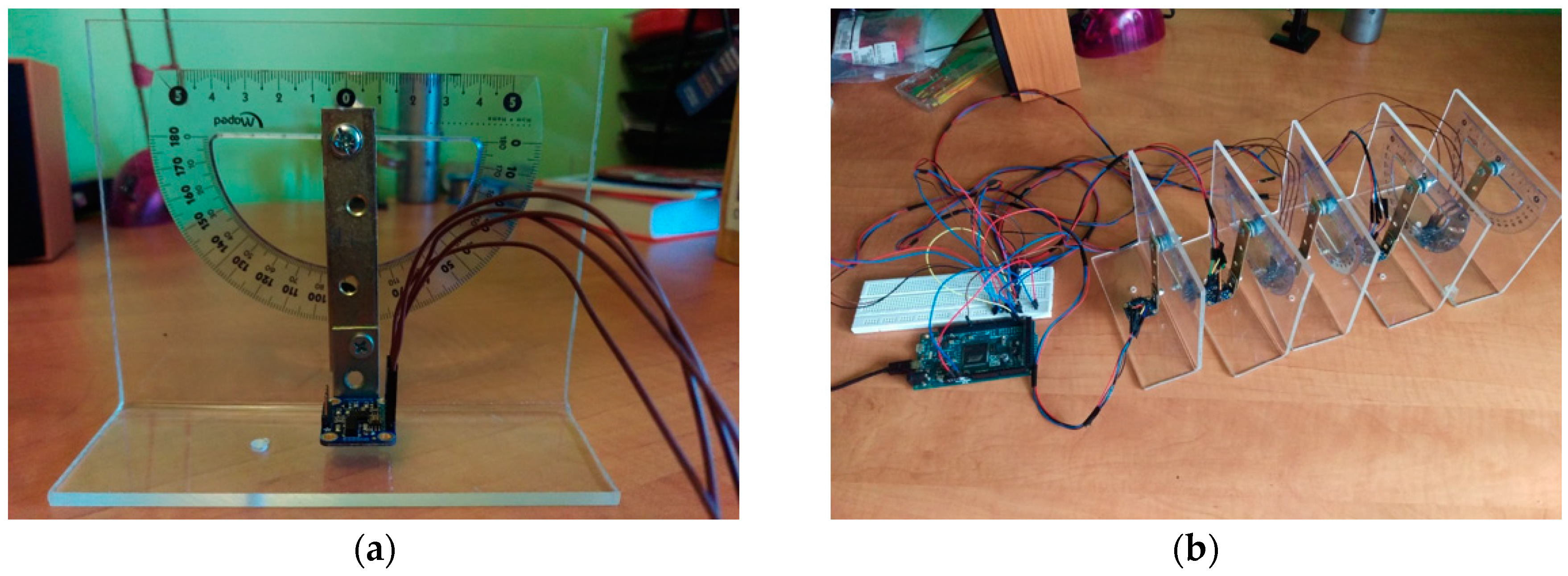
2.1. Measurement System
2.2. Mathematical Model of the Spine
- A mathematical model based on polynomial functions: a 7th grade polynomial is required that is not time and computational efficient.
- A mathematical model based on spline functions: cubic functions for each segment. In this case, we ended with a nonlinear sistem of equations that we found to be difficult to use.
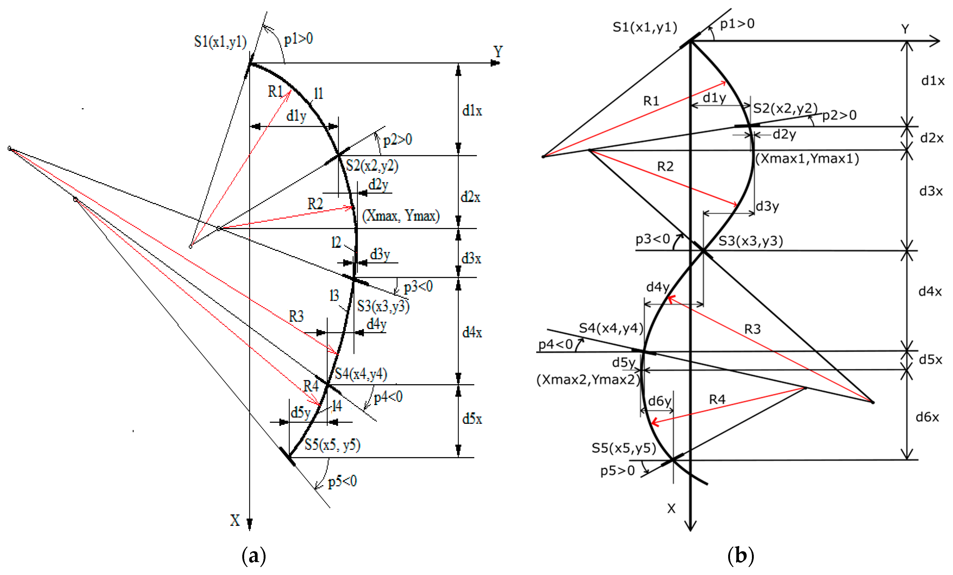
- A mathematical model based on circle arcs (Figure 4): the equations needed to calculate the radius and the coordinates of the imu sensors are only first grade relations. Thus, we get to a linear system of equations that is easier and faster to resolve.
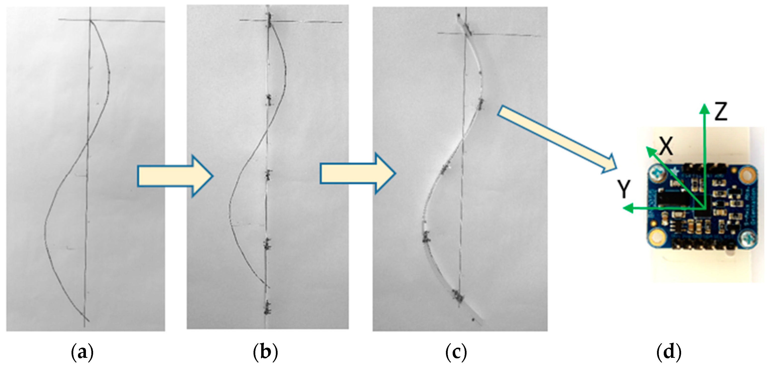
- The wearable monitoring system provides orientation in 3-axis, but we are only using one axis (using all the axes is the subject of another research article).
- The proposed mathematical model is based on the approximation of the real curves with circle arcs and geometrical functions.
- The inputs of the model are the distances measured between the sensors on the flexible frame. The orientation angles are provided by the inertial sensors.
- The segments formed between two sensors are approximated with arcs of length l1, l2, l3, l4 and radius R1, R2, R3, R4. The circle arcs can have different radius, which in the common point have the same tangent to the slope that is equal with the measured value from the inertial sensors.
- The circle arcs will be tangent to each other and a smooth curve will be obtained.
- Determine the length of the circle arcs generated between two successive sensors: l1, l2, l3 and l4 based on radius (R1, R2, R3, R4) and measured angles (p1, p2, p3, p4, p5);
- Calculate the distances on X and Y axis for each sensor, except for the first, which is considered a reference: (d1x, d1y), (d2x, d2y), (d3x, d3y), (d4x, d4y), (d5x, d5y);
- Solve the linear system of 14 equations (Equations (1)–(7) from Table 1) with 14 unknowns (R1, R2, R3, R4, d1x, d1y, d2x, d2y, d3x, d3y, d4x, d4y, d5x, d5y);
- Calculate the (X, Y) coordinates for each sensor (x2, y2), (x3, y3), (x4, y4) and (x5, y5) and for maximum point (Xmax, Ymax);
- Calculate the coordinates of the circle center corresponding to the four arcs (see Table 1).
- The distance between the inertial sensors must be equal (and known), depending on the length of the spine;
- The position of the first sensor to be at the C7 vertebrae, which in general can be easily palpated;
- The prototype must be in contact with the skin. In the lumbar area of the spine, where there is a more pronounced curve, a flexible strap with a soft material can be used to push the sensing array closer to the spine.
2.3. Simulation of Mathematical Model
2.4. Hardware Equipment Analysis
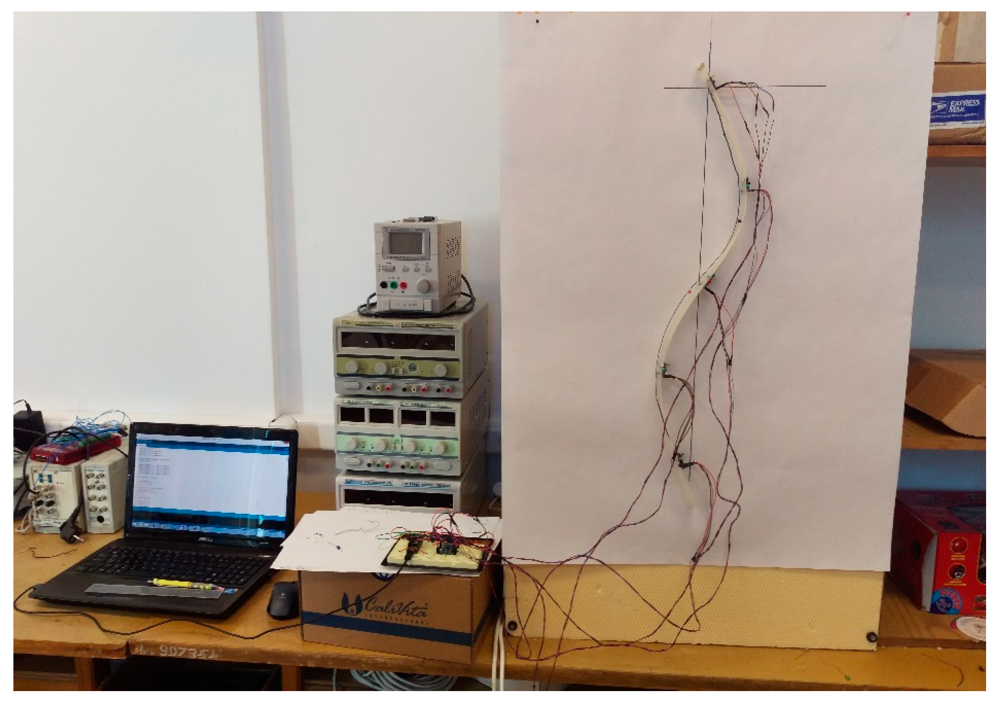
2.4.1. Testing the Acquisition Board
2.4.2. Testing the Sensors
2.4.3. Testing the Wireless Communication
2.4.4. Testing the Local Data Storage
2.5. Measurement Protocol
2.6. Testing Methodology and Results
2.6.1. C2 Posture
2.6.2. A4 Posture
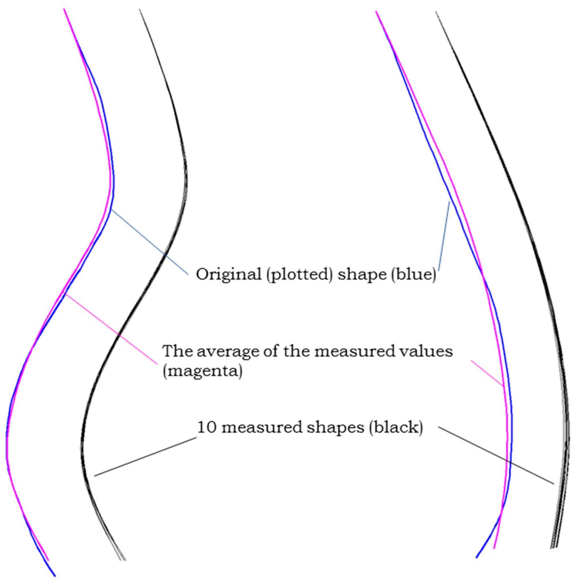
2.7. Visual Representation of Obtained Measurements
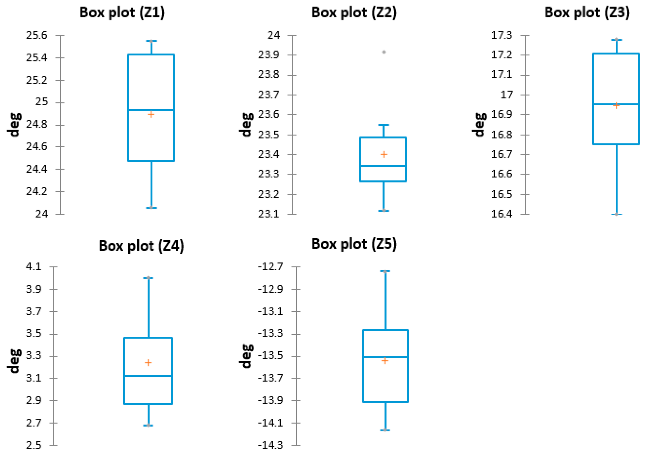
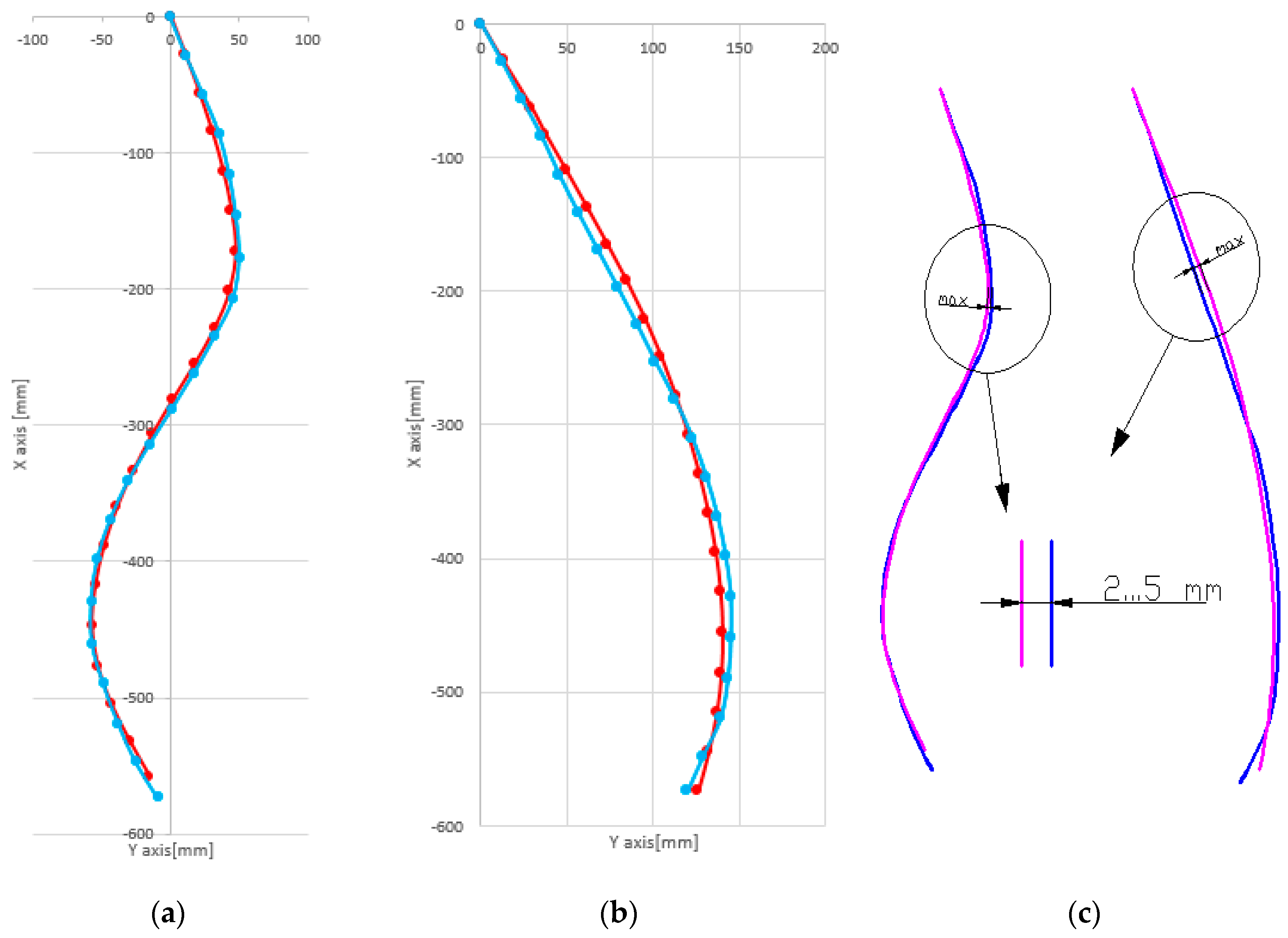
Error assessment
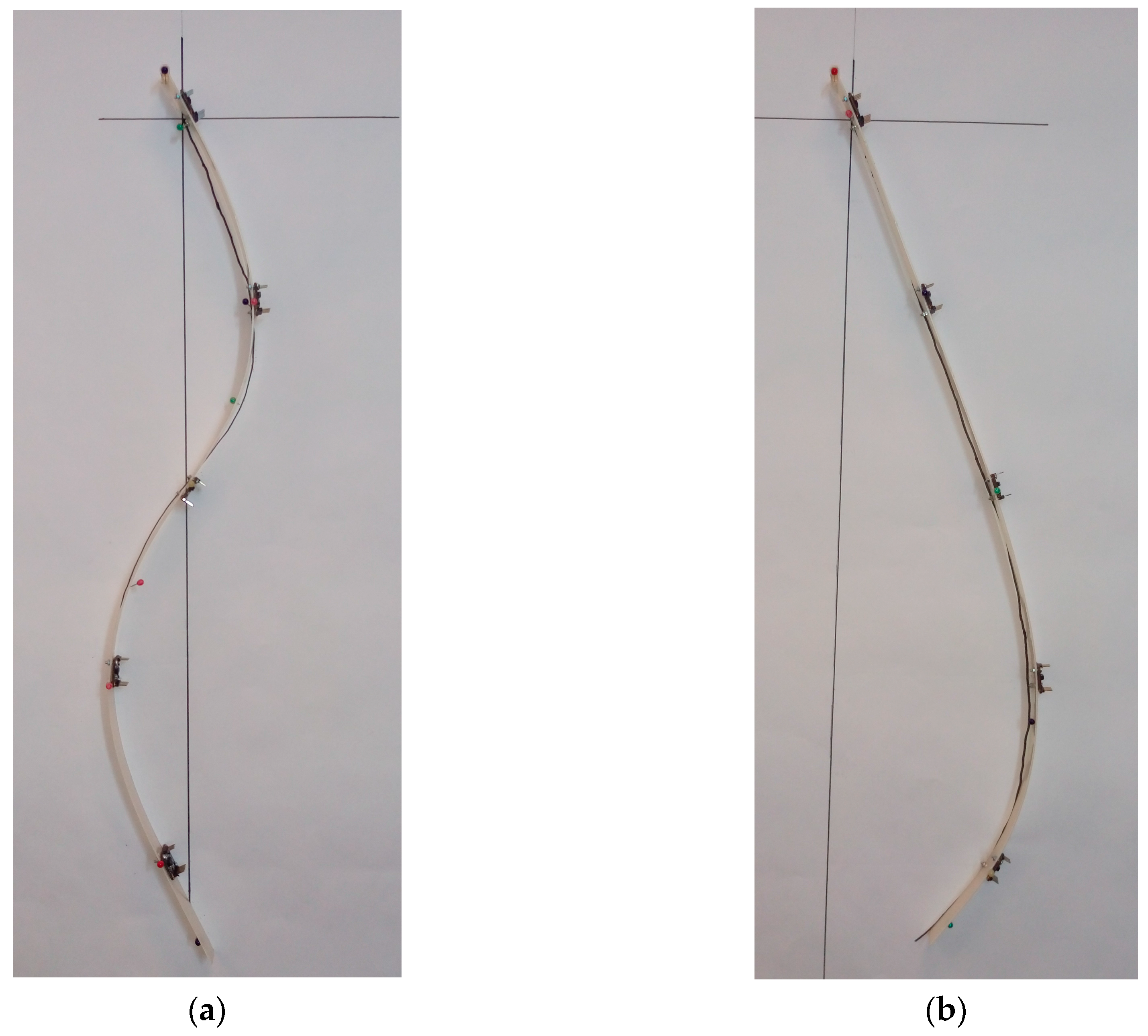
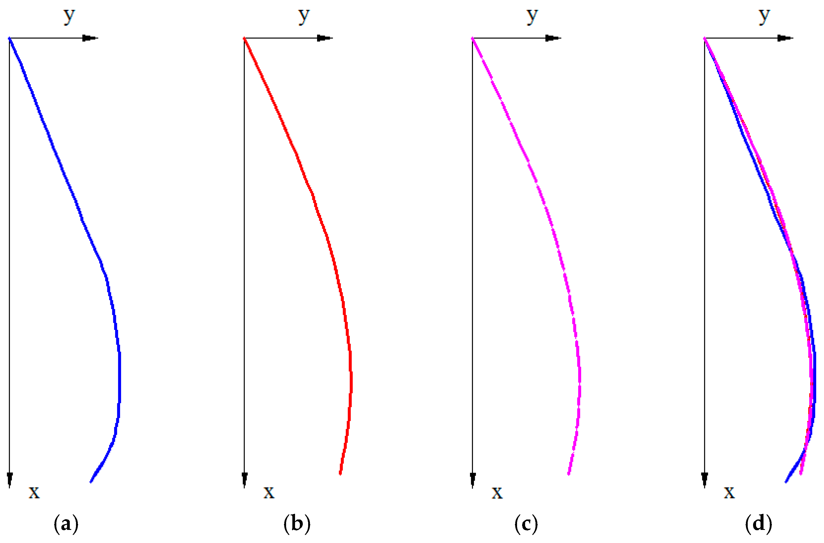
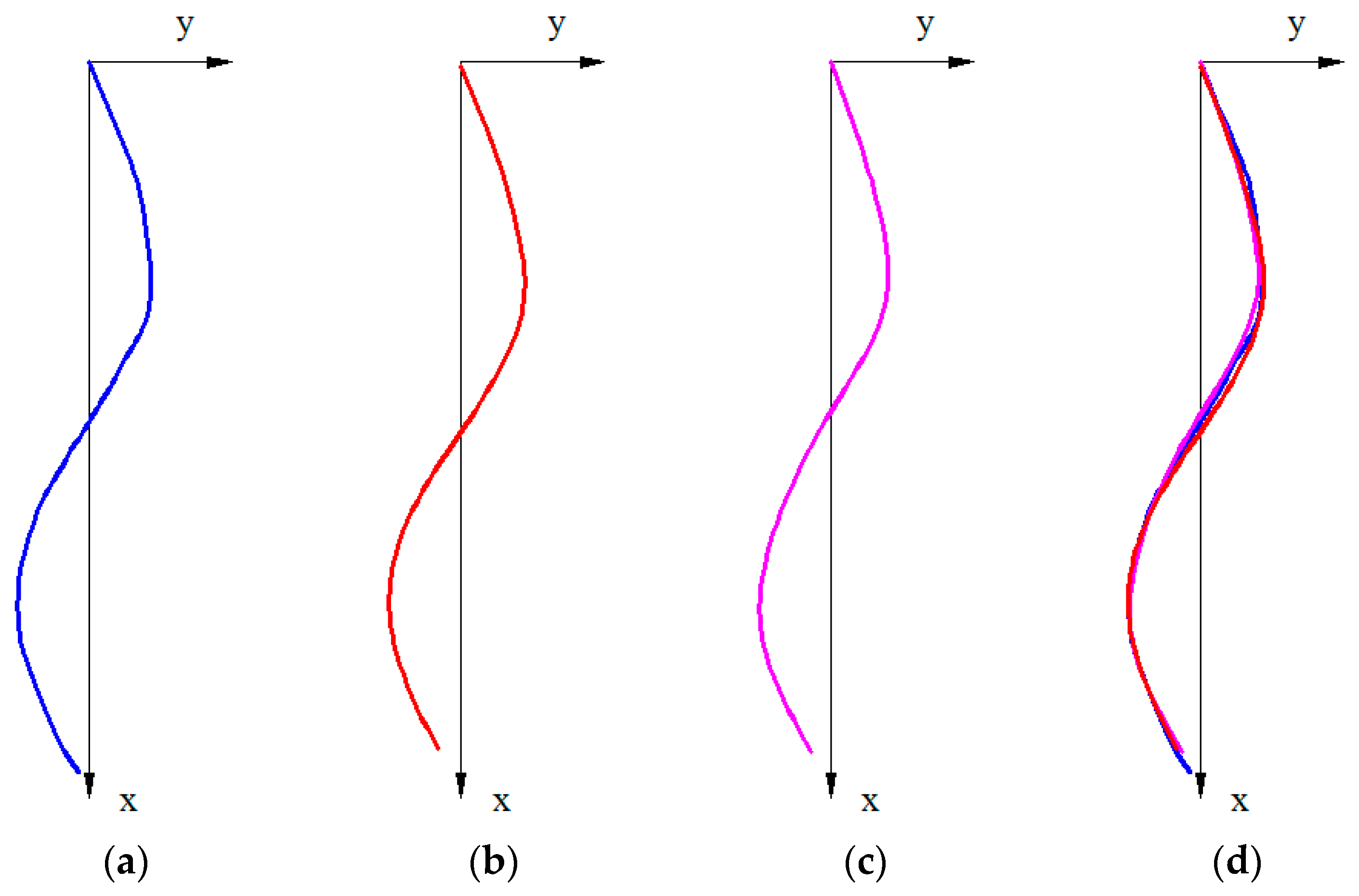
- The spine monitoring system is positioned in a C and S-shape corresponding to models A4 and C2;
- The orientation angles from the inertial sensors are given to the simulation software in which the mathematical model is implemented;
- The mathematical model calculates the coordinates of the sensors;
- The real coordinates of the sensors are manually measured on the testing table;
- We analyze the results from the simulation software with the manually measured distances.
3. Conclusions
Acknowledgments
Author Contributions
Conflicts of Interest
Appendix A

| Name | Criteria | Results |
|---|---|---|
| A1 | Max point between P2 and P3; p1 > p2, p2 < p3, p3 < p4, p4 < p5. |  |
| A2 | Max point between P3 and P4; p1 > p2, p2 > p3, p3 < p4, p4 < p5. |  |
| A3 | Max point between P1 and P2; p1 > p2, p2 < p3, p3 < p4, p4 < p5. |  |
| A4 | Max point between P4 and P5; p1 > p2, p2 > p3, p3 > p4, p4 < p5. |  |
| B1 | Max point between P2 and P3; p1 > p2, p2 < p3, p3 < p4, p4 < p5. |  |
| B2 | Max point between P3 and P4; p1 > p2, p2 > p3, p3 < p4, p4 < p5. |  |
| B3 | Max point between P1 and P2; p1 > p2, p2 < p3, p3 < p4, p4 < p5. |  |
| B4 | Max point between P4 and P5; p1 > p2, p2 > p3, p3 > p4, p4 < p5. |  |
| C1 | Max point between P1-P2 and P3-P4; p1 > p2, p2 < p3, p3 > p4, p4 < p5. |  |
| C2 | Max point between P2-P3 and P4-P5; p1 > p2, p2 < p3, p3 > p4, p4 < p5. |  |
| C3 | Max point between P1-P2 and P3-P4; p1 > p2, p2 < p3, p3 > p4, p4 < p5. |  |
| D1 | Max point between P1-P2 and P3-P4; p1 > p2, p2 < p3, p3 > p4, p4 < p5. |  |
| D2 | Max point between P2-P3 and P4-P5; p1 > p2, p2 < p3, p3 > p4, p4 < p5. |  |
| D3 | Max point between P1-P2 and P3-P4; p1 > p2, p2 < p3, p3 > p4, p4 < p5. |  |
References
- Devedžić, G.; Ćuković, S.; Luković, V.; Milošević, D.; Subburaj, K.; Luković, T. ScolioMedIS: Web-oriented information system for idiopathic scoliosis visualization and monitoring. Comput. Meth. Program. Biomed. 2012, 108, 736–749. [Google Scholar] [CrossRef] [PubMed]
- Humbert, L.; De Guise, J.A.; Aubert, B.; Godbout, B.; Parent, S.; Mitton, D.; Skalli, W. 3D Reconstruction of the Spine from Biplanar X-rays Using Longitudinal and Transversal Inferences. J. Biomech. 2007, 40, S160. [Google Scholar] [CrossRef]
- Lecron, F.; Benjelloun, M.; Mahmoudi, S. Cervical spine mobility analysis on radiographs: A fully automatic approach. Comput. Med. Imaging Grap. 2012, 36, 634–642. [Google Scholar] [CrossRef] [PubMed]
- Milenkovic, S.M.; Kocijancic, R.I.; Belojevic, G.A. Left handedness and spine deformities in early adolescence. Eur. J. Epidemiol. 2004, 19, 969–972. [Google Scholar] [CrossRef] [PubMed]
- Vrtovec, T.; Likar, B.; Pernus, F. Quantitative analysis of spinal curvature in 3D: Application to CT images of normal spine. Phys. Med. Biol. 2008, 53, 1895–1908. [Google Scholar] [CrossRef] [PubMed]
- Salem, W.; Lenders, C.; Mathieu, J.; Hermanus, N.; Klein, P. In vivo three-dimensional kinematics of the cervical spine during maximal axial rotation. Man. Ther. 2013, 18, 339–344. [Google Scholar] [CrossRef] [PubMed]
- Mannion, A.F.; Knecht, K.; Balaban, G.; Dvorak, J.; Grob, D. A new skin-surface device for measuring the curvature and global and segmental ranges of motion of the spine: Reliability of measurements and comparison with data reviewed from the literature. Eur. Spine J. 2004, 13, 122–136. [Google Scholar] [CrossRef] [PubMed]
- Plamondon, A.; Delisle, A.; Larue, C.; Brouillette, D.; Mcfadden, D.; Desjardins, P.; Larivière, C. Evaluation of a hybrid system for three-dimensional measurement of trunk posture in motion. Appl. Ergon. 2007, 38, 697–712. [Google Scholar] [CrossRef] [PubMed]
- Kadoury, S.; Labelle, H.; Paragios, N. Automatic inference of articulated spine models in CT images using high-order Markov Random Fields. Med. Image Anal. 2011, 15, 426–437. [Google Scholar] [CrossRef] [PubMed]
- Laurent, C.P.; Jolivet, E.; Hodel, J.; Decq, P.; Skalli, W. New method for 3D reconstruction of the human cranial vault from CT-scan data. Med. Eng. Phys. 2011, 33, 1270–1275. [Google Scholar] [CrossRef] [PubMed]
- Reutlinger, C.; Gedet, P.; Buchler, P.; Kowal, J.; Rudolph, T.; Burger, J.; Scheffler, K.; Hasler, C. Combining 3D tracking and surgical instrumentation to determine the stiffness of spinal motion segments: A validation study. Med. Eng. Phys. 2011, 33, 340–346. [Google Scholar] [CrossRef] [PubMed]
- Yamauchi, T.; Yamazaki, M.; Okawa, A.; Furuya, T.; Hayashi, K.; Sakuma, T.; Takahashi, H.; Yanagawa, N.; Koda, M. Efficacy and reliability of highly functional open source DICOM software (OsiriX) in spine surgery. J. Clin. Neurosci. 2010, 17, 756–759. [Google Scholar] [CrossRef] [PubMed]
- Ranavolo, A.; Don, R.; Draicchio, F.; Bartolo, M.; Serrao, M.; Padua, L.; Cipolla, G.; Pierelli, F.; Iavicoli, S.; Sandrini, G. Modelling the spine as a deformable body: Feasibility of reconstruction using an optoelectronic system. Appl. Ergon. 2013, 44, 192–199. [Google Scholar] [CrossRef] [PubMed]
- Schmid, S.; Studer, D.; Hasler, C.C.; Romkes, J.; Taylor, W.R.; Lorenzetti, S.; Brunner, R. Quantifying spinal gait kinematics using an enhanced optical motion capture approach in adolescent idiopathic scoliosis. Gait Posture 2016, 44, 231–237. [Google Scholar] [CrossRef] [PubMed]
- Berthonnaud, E.; Dimnet, J.; Roussouly, P.; Labelle, H. Analysis of the sagittal balance of the spine and pelvis using shape and orientation parameters. J. Spinal Disord. Tech. 2005, 18, 40–47. [Google Scholar] [CrossRef] [PubMed]
- Meakin, J.R.; Gregory, J.S.; Smith, F.W.; Gilbert, F.J.; Aspden, R.M. Characterizing the shape of the lumbar spine using an active shape model: Reliability and precision of the method. Spine 2008, 33, 807–813. [Google Scholar] [CrossRef] [PubMed]
- Tillotson, K.M.; Burton, A.K. Noninvasive measurement of lumbar sagittal mobility. An assessment of the flexicurve technique. Spine 1991, 16, 29–33. [Google Scholar] [CrossRef] [PubMed]
- Remondino, F. 3-D reconstruction of static human body shape from image sequence. Comput. Vis. Image Underst. 2004, 93, 65–85. [Google Scholar] [CrossRef]
- Jia, W.; Yi, W.J.; Saniie, J.; Oruklu, E. 3D image reconstruction and human body tracking using stereo vision and Kinect technology. In Proceedings of the 2012 IEEE International Conference on Electro/Information Technology (EIT), Indianapolis, IN, USA, 6–8 May 2012; pp. 1–4.
- Li, Z.; Jia, W.; Mao, Z.H.; Li, J.; Chen, H.C.; Zuo, W.; Wang, K.; Sun, M. Anthropometric body measurements based on multi-view stereo image reconstruction. In Proceedings of the 2013 35th Annual International Conference of the IEEE Engineering in Medicine and Biology Society (EMBC), Osaka, Japan, 3–7 July 2013; pp. 366–369.
- Yang, H.D.; Lee, S.W. Reconstruction of 3D human body pose from stereo image sequences based on top-down learning. Pattern Recognit. 2007, 40, 3120–3131. [Google Scholar] [CrossRef]
- Consmüller, T.; Rohlmann, A.; Weinland, D.; Druschel, C.; Duda, G.N. Comparative evaluation of a novel measurement tool to assess lumbar spine posture and range of motion. Eur. Spine J. 2012, 21, 2170–2180. [Google Scholar] [CrossRef] [PubMed]
- Dreischarf, M.; Pries, E.; Bashkuev, M.; Putzier, M.; Schmidt, H. Differences between clinical “snap-shot” and “real-life” assessments of lumbar spine alignment and motion – What is the “real” lumbar lordosis of a human being? J. Biomech. 2016, 49, 638–644. [Google Scholar] [CrossRef] [PubMed]
- Taylor, W.R.; Consmüller, T.; Rohlmann, A. A novel system for the dynamic assessment of back shape. Med. Eng. Phys. 2010, 32, 1080–1083. [Google Scholar] [CrossRef] [PubMed]
- Motion Capture Systems Vicon. Available online: http://www.vicon.com/ (accessed on 18 August 2016).
- O’Sullivan, K.; O’Sullivan, L.; Campbell, A.; O’Sullivan, P.; Dankaerts, W. Towards monitoring lumbo-pelvic posture in real-life situations: Concurrent validity of a novel posture monitor and a traditional laboratory-based motion analysis system. Man. Ther. 2012, 17, 77–83. [Google Scholar] [CrossRef] [PubMed]
- Mieritz, R.M.; Bronfort, G.; Jakobsen, M.D.; Aagaard, P.; Hartvigsen, J. Reliability and measurement error of sagittal spinal motion parameters in 220 chronic low back pain patients using a 3D measurement device. Spine J. 2014, 14, 1835–1843. [Google Scholar] [CrossRef] [PubMed]
- Petersen, C.M.; Schuit, D.; Johnson, R.D.; Knecht, H.; Levine, P. Agreement of measures obtained radiographically and by the OSI CA-6000 Spine Motion Analyzer for cervical spinal motion. Man. Ther. 2008, 13, 200–205. [Google Scholar] [CrossRef] [PubMed]
- Verhaert, V.; Druyts, H.; Van Deun, D.; Exadaktylos, V.; Verbraecken, J. Estimating spine shape in lateral sleep positions using silhouette-derived body shape models. Int. J. Ind. Ergon. 2012, 42, 489–498. [Google Scholar] [CrossRef]
- Goodvin, C.; Park, E.J.; Huang, K.; Sakaki, K. Development of a real-time three-dimensional spinal motion measurement system for clinical practice. Med. Biol. Eng. Comput. 2006, 44, 1061–1075. [Google Scholar] [CrossRef] [PubMed]
- Lee, J.K.; Desmoulin, G.T.; Khan, A.H.; Park, E.J. Comparison of 3D spinal motions during stair-climbing between individuals with and without low back pain. Gait Posture 2011, 34, 222–226. [Google Scholar] [CrossRef] [PubMed]
- Theobald, P.S.; Jones, M.D.; Williams, J.M. Do inertial sensors represent a viable method to reliably measure cervical spine range of motion? Man. Ther. 2011, 17, 92–96. [Google Scholar] [CrossRef] [PubMed]
- Williams, J.M.; Haq, I.; Lee, R.Y. Dynamic measurement of lumbar curvature using fibre-optic sensors. Med. Eng. Phys. 2010, 32, 1043–1049. [Google Scholar] [CrossRef] [PubMed]
- Wunderlich, M.; Rüther, T.; Essfeld, D.; Erren, T.C.; Piekarski, C.; Leyk, D. A new approach to assess movements and isometric postures of spine and trunk at the workplace. Eur. Spine J. 2011, 20, 1393–1402. [Google Scholar] [CrossRef] [PubMed]
- Roussouly, P.; Nnadi, C. Sagittal Plane Deformity: An Overview of Interpretation and Management. Eur. Spine J. 2010, 19, 1824–1836. [Google Scholar] [CrossRef] [PubMed]
- Devedžić, G.; Stojanović, R.; Luković, V.; Ćuković, S.; Milošević, D. Identification of anatomical landmarks for intelligent postural sensing. In Proceedings of the 2012 Mediterranean Conference on Embedded Computing (MECO), Bar, Montenegro, 19–21 June 2012; pp. 70–73.
- Maplesoft Technical Computing Software. Available online: http://www.maplesoft.com/ (accessed on 18 June 2016).
- SparkFun Bluetooth Mate Silver. Available online: https://www.sparkfun.com/products/12576 (accessed on 10 April 2016).
- Arduino & Rasberry PI GSM/GPRS/SMS/DTMF Shield. Available online: http://itbrainpower.net/a-gsm (accessed on 5 April 2016).
- Statistical Software for Excel. Available online: https://www.xlstat.com/en/ (accessed on 23 June 2016).


| Single Max Point Curve (“C” Shape) | Double Max Point Curve (“S” Shape) | Equation Number |
|---|---|---|
| (1) | ||
| (2) | ||
| (3) | ||
| (4) | ||
| (5) | ||
| (6) | ||
| (7) | ||
| (8) | ||
| (9) | ||
| (10) | ||
| (11) | ||
| (12) | ||
| (13) | ||
| (14) | ||
| (15) | ||
| (16) | ||
| (17) |
| Name | Criteria | Results |
|---|---|---|
| A4 | Max point between P4 and P5; p1 > p2, p2 > p3, p3 > p4, p4 < p5. |  |
| C2 | Max point between P2-P3 and P4-P5; p1 > p2, p2 < p3, p3 > p4, p4 < p5. |  |
| Characteristic | Bosch BNO055 | MPU 9150 | Flora LSM9DS0 | AltIMU 10 v.4 | MinIMU 9 V3 |
|---|---|---|---|---|---|
| Accelerometer | |||||
| Measurement range | ±2 g to ±16 g | ±2 g to ±16 g | ±2 g to ±16 g | ±2 g to ±16 g | ±2 g to ±16 g |
| Sensitivity | 1 LSB/g | 2 LSB/g | 0.732 LSB/g | 0.732 LSB/g | 0.732 LSB/g |
| Gyroscope | |||||
| Measurement range | ±125°/s to ±2000°/s | ±250°/s to ±2000°/s | ±245°/s to ±2000°/s | ±245°/s to ±2000°/s | ±245°/s to ±2000°/s |
| Sensitivity | 16 LSB/°/s | 16.4 LSB/°/s | 70 LSB/°/s | 70 LSB/°/s | 70 LSB/°/s |
| Magnetometer | |||||
| Measurement range | ±1300 μT (x-, y-axis); ±2500 μT (z-axis) | ±1200 µT | 200 µT to 1200 µT | 200 µT to 1200 µT | 200 µT to 1200 µT |
| Resolution | 0.3 μT | 0.3 μT | 0.48 μT | 0.47 μT | 0.47 μT |
| Temperature sensor | Yes | Yes | Yes | No, includes a 24 bits barometer | No |
| Size (mm) | 20 × 27 × 4 | 15.5 × 29 × 4 | Diameter of 16 mm, Width 0.8 mm | 25.4 × 12.7 × 2.54 | 20 × 13 × 3 |
| Communication | HID-I2C/I2C/UART | I2C | SPI/I2C | I2C | I2C |
| Supply voltage | 2.4 V to 3.6 V | 2.4 V to 3.46 V | 2.4 V to 3.6 V | 2.5 V to 5.5 V | 2.5 V to 5.5 V |
| Power management | Yes, with three modes | No | Yes | No | No |
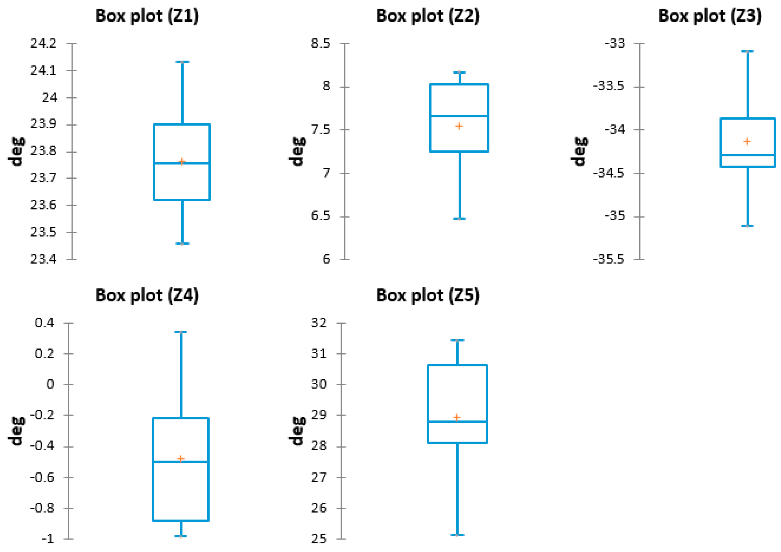
| Statistic | Z1 | Z2 | Z3 | Z4 | Z5 |
|---|---|---|---|---|---|
| Nbr. of observations | 10 | 10 | 10 | 10 | 10 |
| Minimum | 23.460 | 6.470 | −35.110 | −0.980 | 25.140 |
| Maximum | 24.130 | 8.170 | −33.090 | 0.340 | 31.440 |
| 1st Quartile | 23.620 | 7.253 | −34.423 | −0.878 | 28.123 |
| Median | 23.755 | 7.660 | −34.285 | −0.500 | 28.790 |
| 3rd Quartile | 23.900 | 8.028 | −33.865 | −0.215 | 30.638 |
| Mean | 23.762 | 7.550 | −34.134 | −0.477 | 28.962 |
| Variance (n − 1) | 0.050 | 0.371 | 0.369 | 0.192 | 3.796 |
| Standard deviation (n − 1) | 0.223 | 0.609 | 0.607 | 0.438 | 1.948 |
| Statistic | Z1 | Z2 | Z3 | Z4 | Z5 |
|---|---|---|---|---|---|
| Nbr. of observations | 10 | 10 | 10 | 10 | 10 |
| Minimum | 24.060 | 23.120 | 16.400 | 2.680 | −14.160 |
| Maximum | 25.550 | 23.920 | 17.280 | 4.000 | −12.740 |
| 1st Quartile | 24.475 | 23.265 | 16.750 | 2.870 | −13.908 |
| Median | 24.930 | 23.345 | 16.955 | 3.130 | −13.510 |
| 3rd Quartile | 25.430 | 23.488 | 17.210 | 3.463 | −13.263 |
| Mean | 24.889 | 23.401 | 16.948 | 3.238 | −13.536 |
| Variance (n − 1) | 0.334 | 0.05 | 0.084 | 0.211 | 0.188 |
| Standard deviation (n − 1) | 0.578 | 0.223 | 0.290 | 0.460 | 0.434 |
© 2016 by the authors; licensee MDPI, Basel, Switzerland. This article is an open access article distributed under the terms and conditions of the Creative Commons Attribution (CC-BY) license (http://creativecommons.org/licenses/by/4.0/).
Share and Cite
Voinea, G.-D.; Butnariu, S.; Mogan, G. Measurement and Geometric Modelling of Human Spine Posture for Medical Rehabilitation Purposes Using a Wearable Monitoring System Based on Inertial Sensors. Sensors 2017, 17, 3. https://doi.org/10.3390/s17010003
Voinea G-D, Butnariu S, Mogan G. Measurement and Geometric Modelling of Human Spine Posture for Medical Rehabilitation Purposes Using a Wearable Monitoring System Based on Inertial Sensors. Sensors. 2017; 17(1):3. https://doi.org/10.3390/s17010003
Chicago/Turabian StyleVoinea, Gheorghe-Daniel, Silviu Butnariu, and Gheorghe Mogan. 2017. "Measurement and Geometric Modelling of Human Spine Posture for Medical Rehabilitation Purposes Using a Wearable Monitoring System Based on Inertial Sensors" Sensors 17, no. 1: 3. https://doi.org/10.3390/s17010003