Acknowledgments
This work was supported by the National Key R&D Program (2016YFD0300601), the Fundamental Research Funds for the Central Universities (KYRC201401), the National Natural Science Foundation of China (31470084, 31371535), Jiangsu Distinguished Professor Program, Jiangsu Entrepreneurship and Innovation Doctor Program, Special Program for Agriculture Science and Technology from Ministry of Agriculture in China (201303109), the Academic Program Development of Jiangsu Higher Education Institutions (PAPD) and the Innovation of Graduate Student Training Project in Jiangsu Province (KYLX_0604). K.Z. was supported by a two-year visiting student scholarship from the China Scholarship Council (CSC).
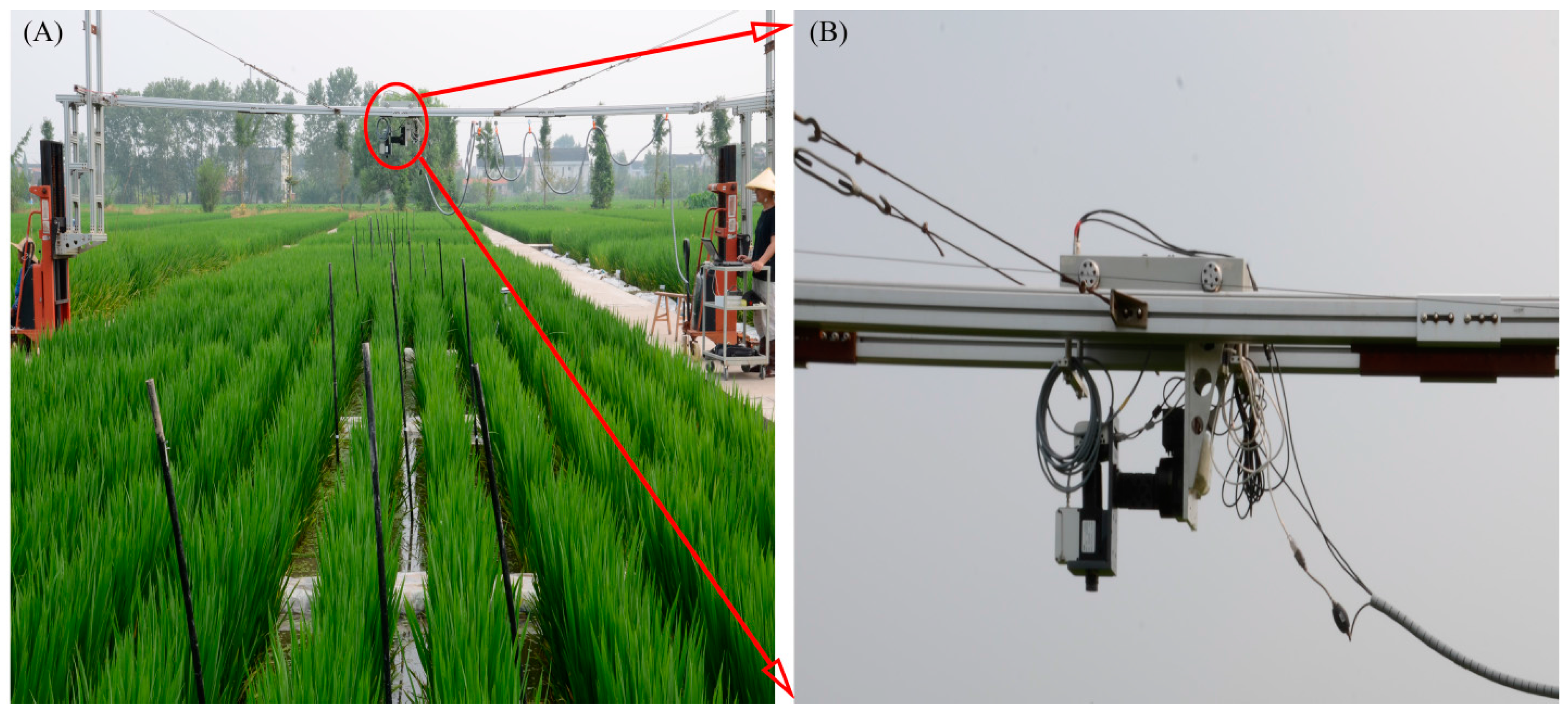
Figure 1.
(A) Setup of the near-ground hyperspectral imaging system in the rice field and (B) onset of the hyperspectral camera in the system.
Figure 1.
(A) Setup of the near-ground hyperspectral imaging system in the rice field and (B) onset of the hyperspectral camera in the system.
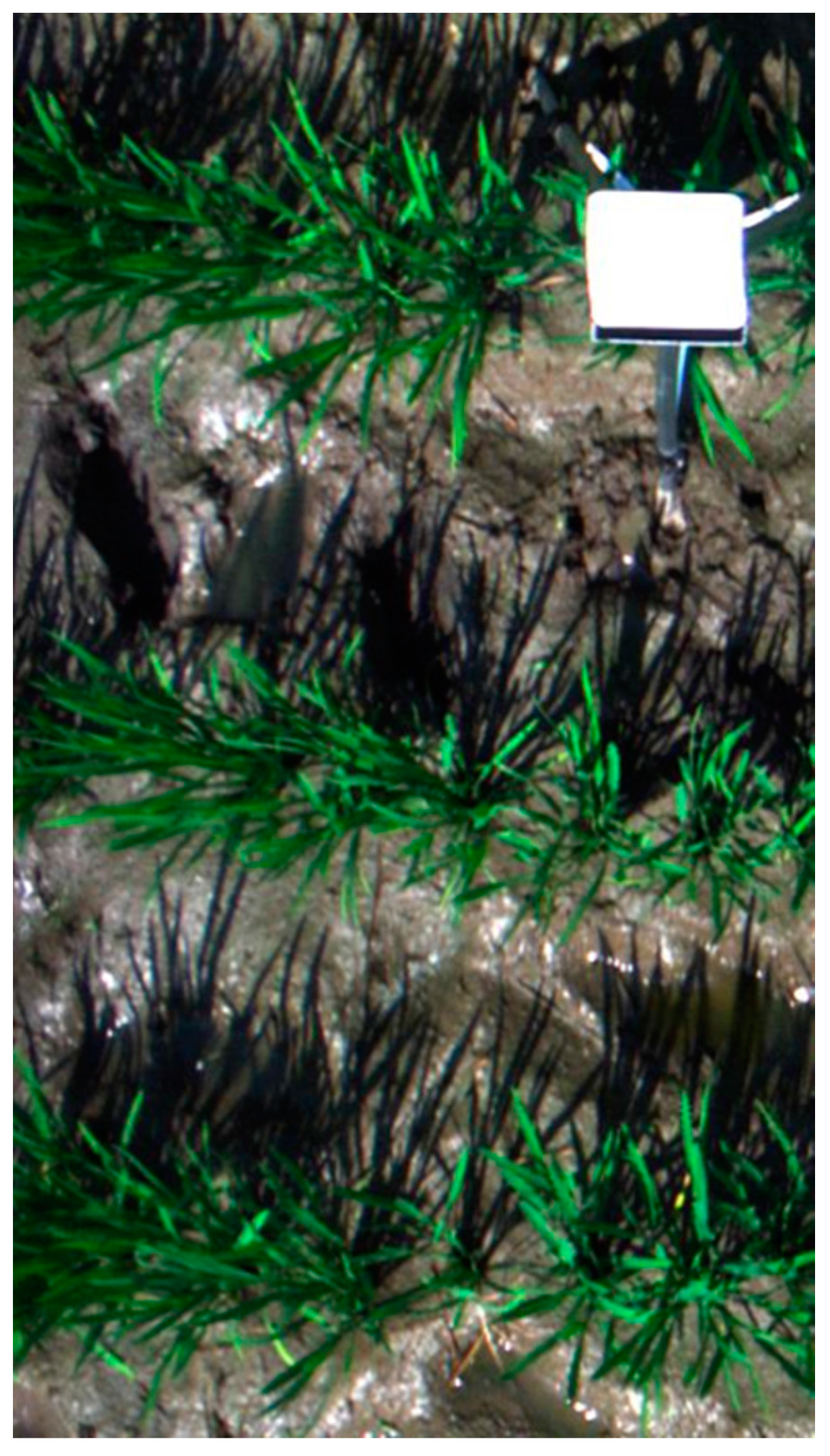
Figure 2.
An example true color image cropped from a hyperspectral scene acquired on 20 July 2014.
Figure 2.
An example true color image cropped from a hyperspectral scene acquired on 20 July 2014.
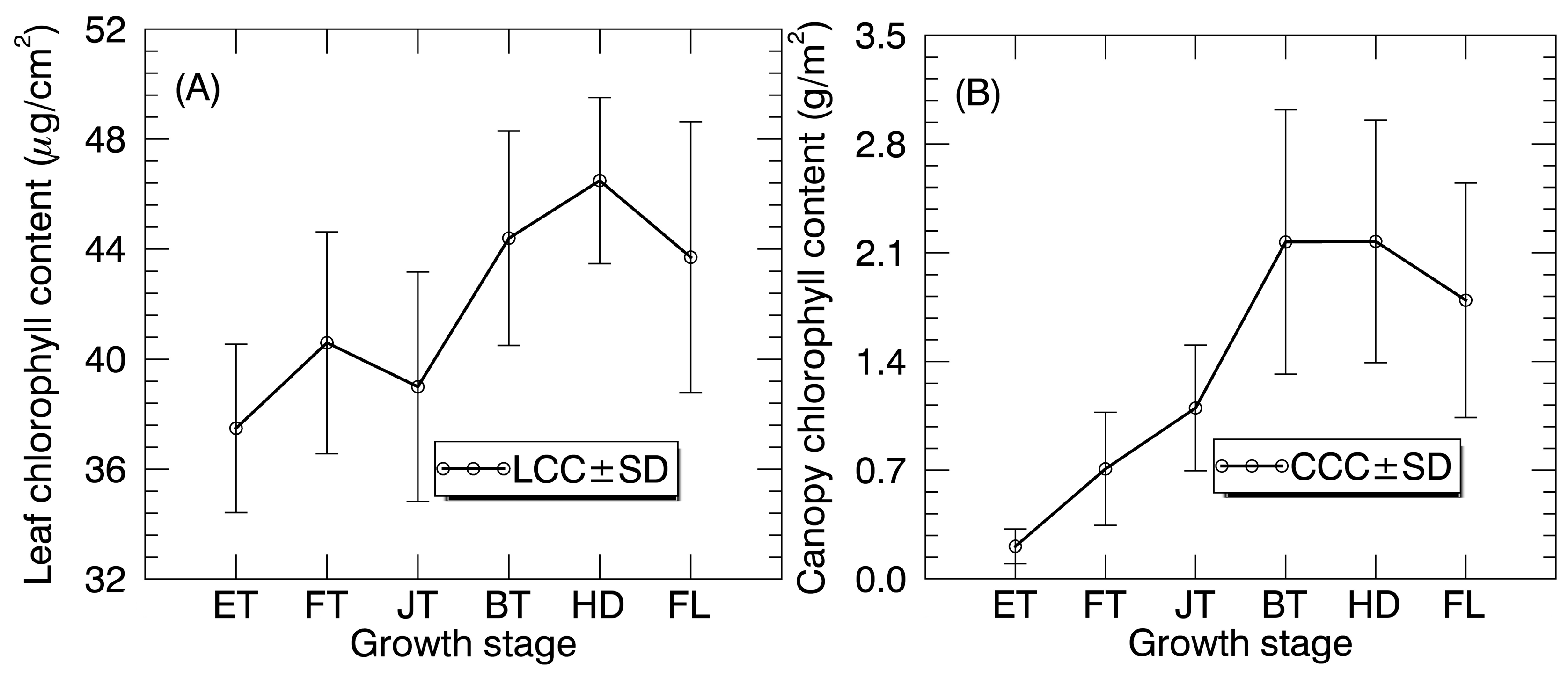
Figure 3.
The temporal profiles of (A) LCC and (B) CCC in paddy rice over the whole growing season. LCC and CCC values are shown as mean ± standard deviation (SD).
Figure 3.
The temporal profiles of (A) LCC and (B) CCC in paddy rice over the whole growing season. LCC and CCC values are shown as mean ± standard deviation (SD).
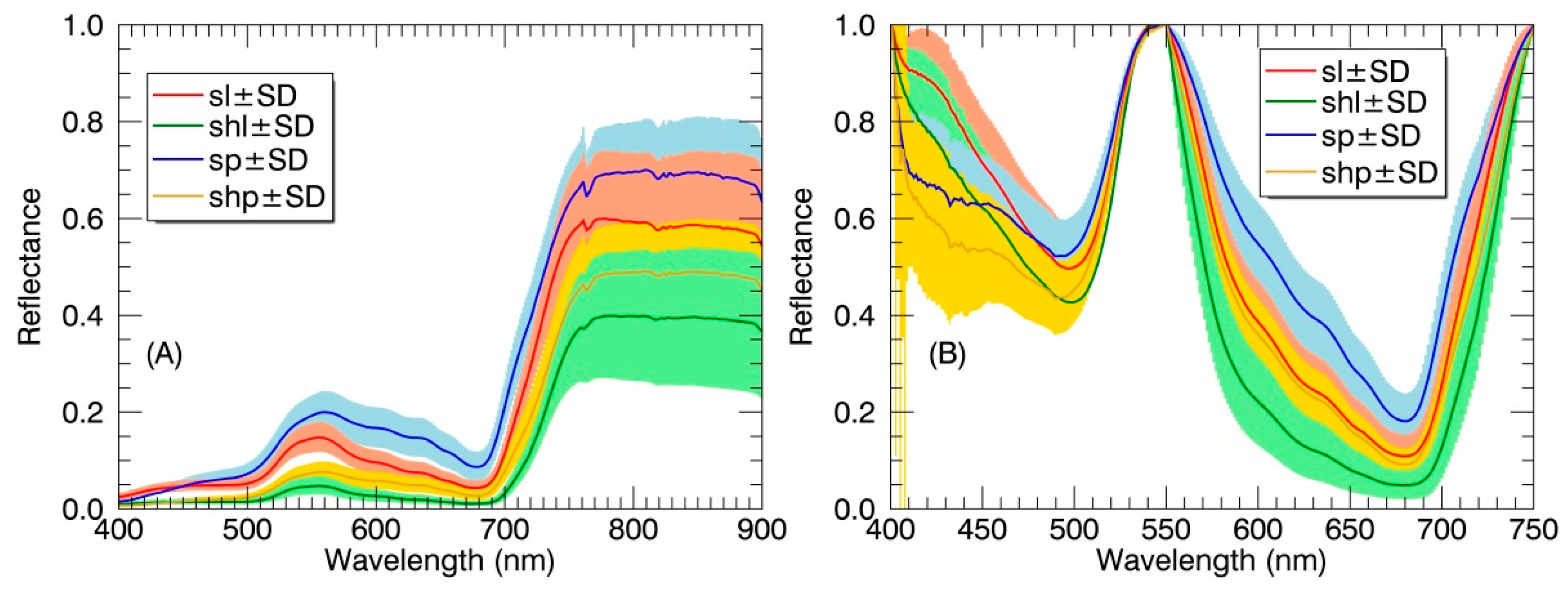
Figure 4.
(A) The reflectance spectra and (B) continuum-removed reflectance spectra of different canopy components in paddy rice over the whole growing season. Spectral values are shown as mean ± standard deviation (SD). SL: sunlit leaf; SHL: shaded leaf; SP: sunlit panicle; SHP: shaded panicle.
Figure 4.
(A) The reflectance spectra and (B) continuum-removed reflectance spectra of different canopy components in paddy rice over the whole growing season. Spectral values are shown as mean ± standard deviation (SD). SL: sunlit leaf; SHL: shaded leaf; SP: sunlit panicle; SHP: shaded panicle.
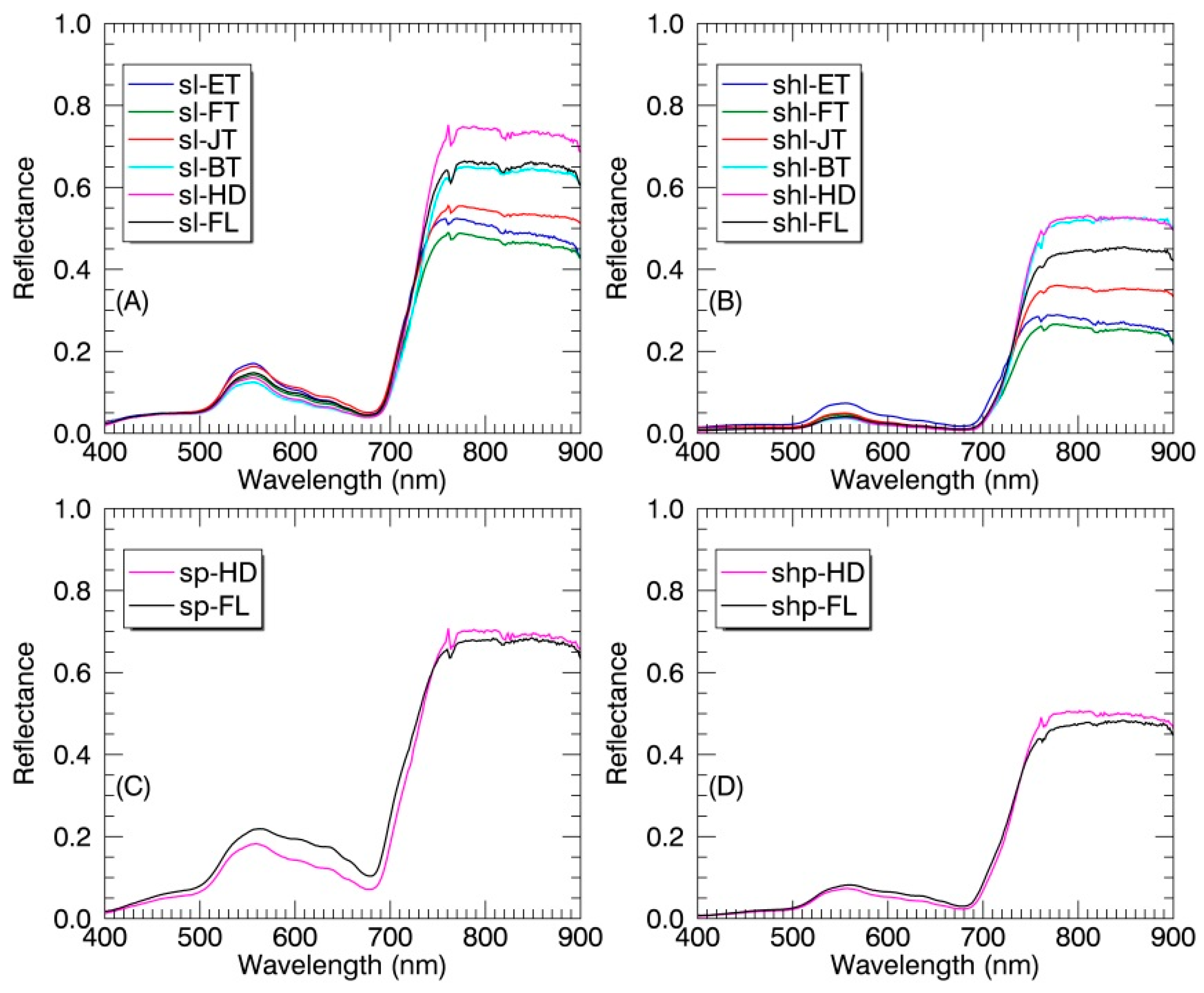
Figure 5.
The average reflectance spectra of SL (A), SHL (B), SP (C) and SHP (D) in paddy rice at individual growth stages. ET: early tillering stage; FT: fully tillering stage; JT: jointing stage; BT: booting stage; HD: heading stage; FL: filling stage.
Figure 5.
The average reflectance spectra of SL (A), SHL (B), SP (C) and SHP (D) in paddy rice at individual growth stages. ET: early tillering stage; FT: fully tillering stage; JT: jointing stage; BT: booting stage; HD: heading stage; FL: filling stage.
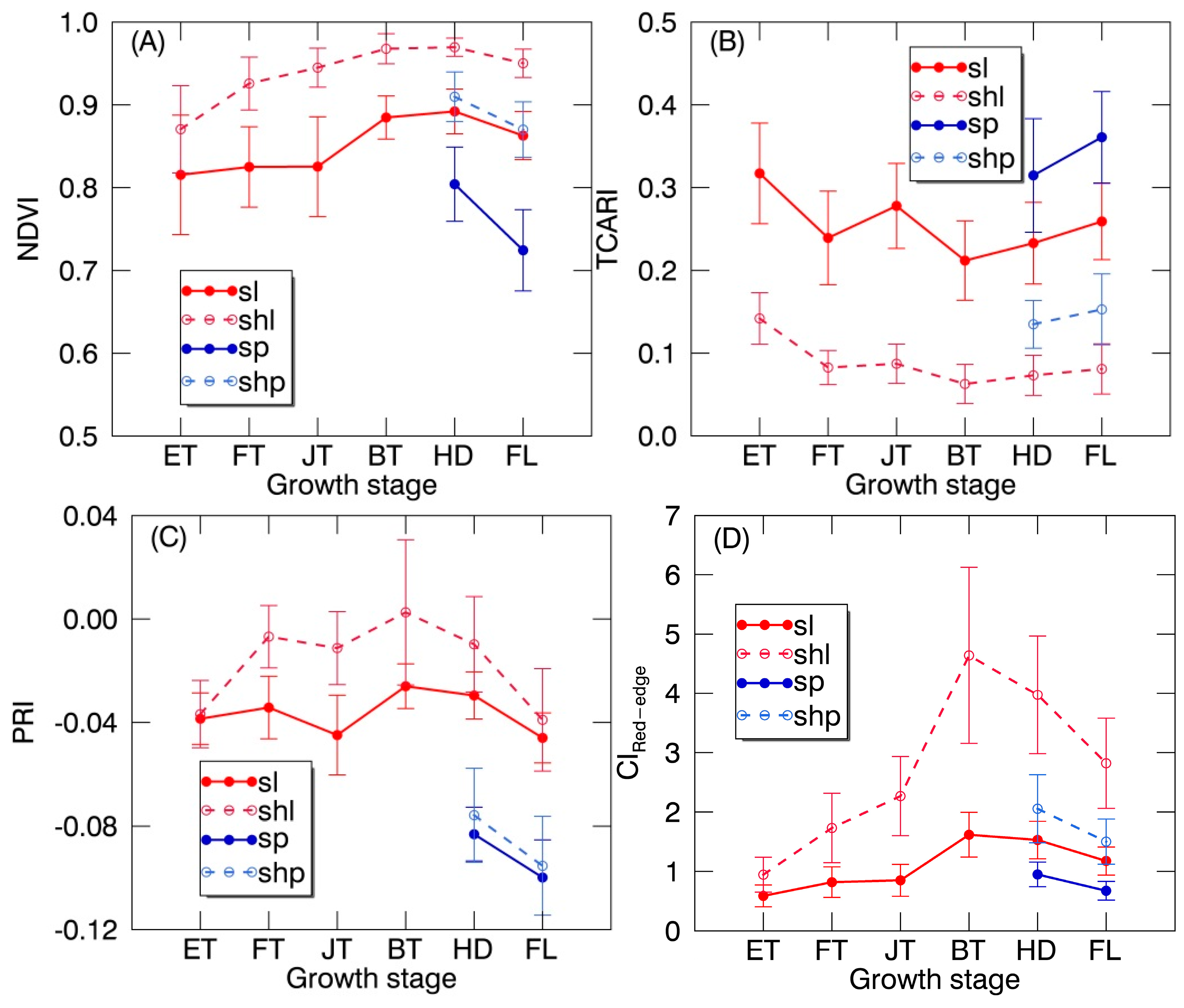
Figure 6.
The temporal profile (mean ± standard deviation) of (A) normalized difference vegetation index (NDVI), (B) transformed chlorophyll absorption reflectance index (TCARI), (C) photochemical reflectance index (PRI) and (D) red edge chlorophyll index (CIRed-edge) derived from regions of interest (ROIs) for SL, SHL, SP and SHP over the whole growing season. ET: early tillering stage; FT: fully tillering stage; JT: jointing stage; BT: booting stage; HD: heading stage; FL: filling stage.
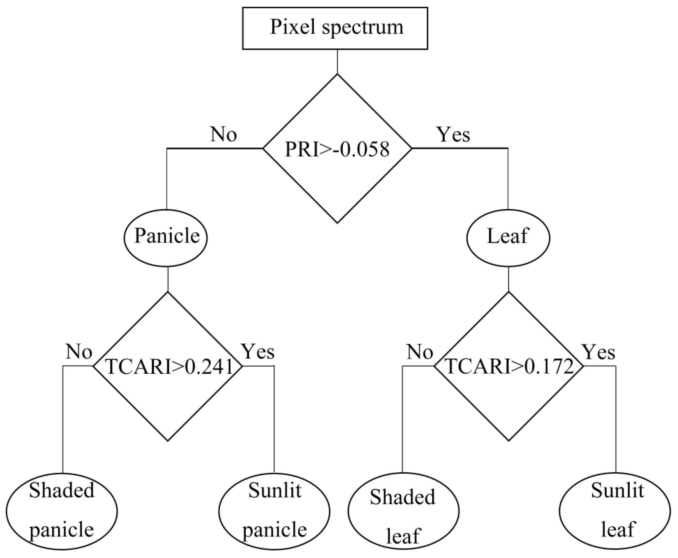
Figure 7.
Decision tree for separating four canopy components: SL; SHL; SP; SHP across all growth stages. Each option (yes or no) leads to a condition or to a classification product. The PRI threshold for separating leaves and panicles was determined as their respective mean PRI values of all the ROIs datasets averaged over the whole growing season. In the same way, the TCARI thresholds for separating SL vs. SHL and SP vs. SHP were determined by averaging their respective mean TCARI values.
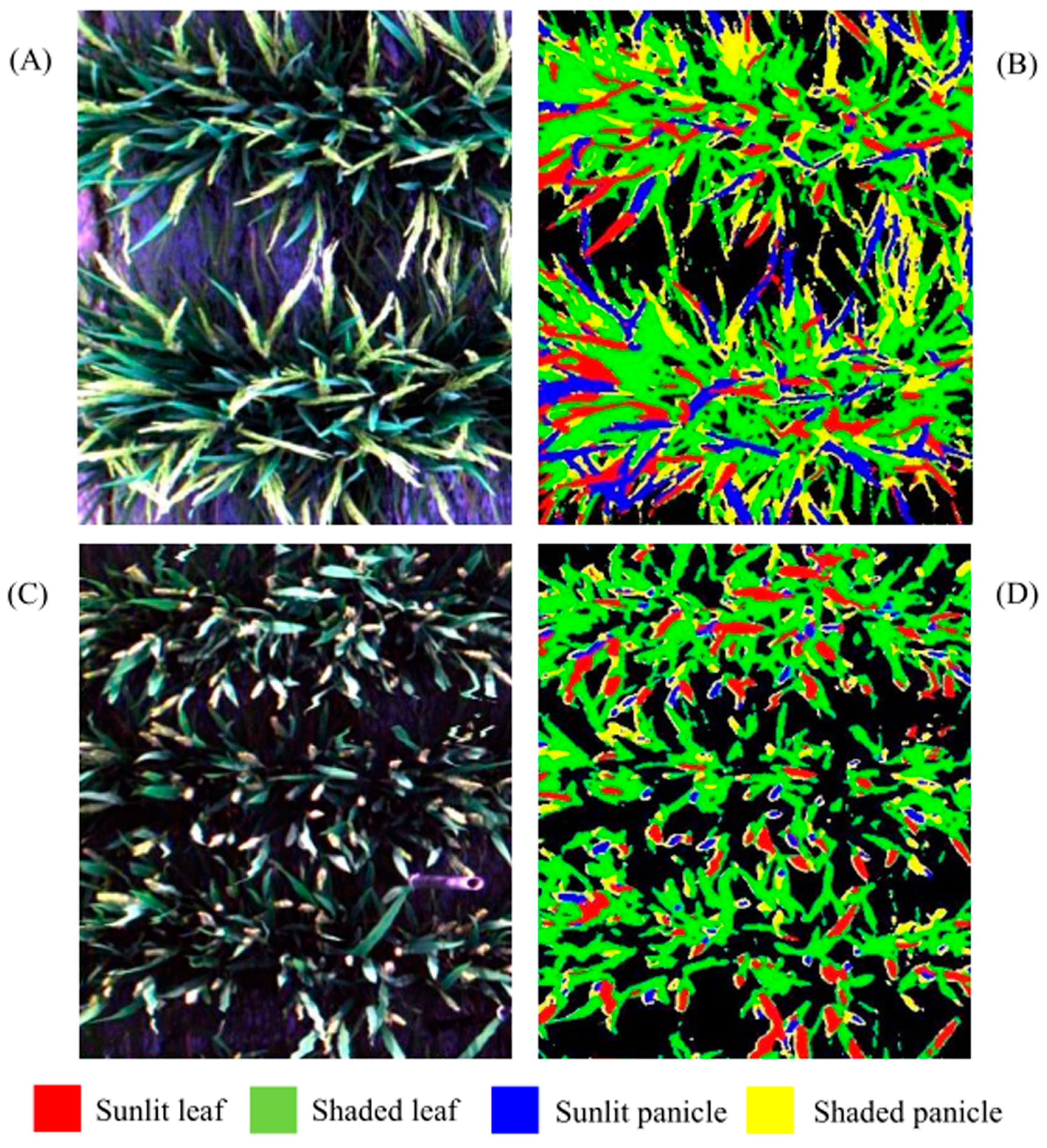
Figure 8.
Two true color composites ((A) Indica rice; (C) Japonica rice) and decision tree classification maps ((B) Indica rice; (D) Japonica rice) for the rice experiment at the heading stage. The black background in (B,D) represents non-vegetation pixels.
Figure 8.
Two true color composites ((A) Indica rice; (C) Japonica rice) and decision tree classification maps ((B) Indica rice; (D) Japonica rice) for the rice experiment at the heading stage. The black background in (B,D) represents non-vegetation pixels.
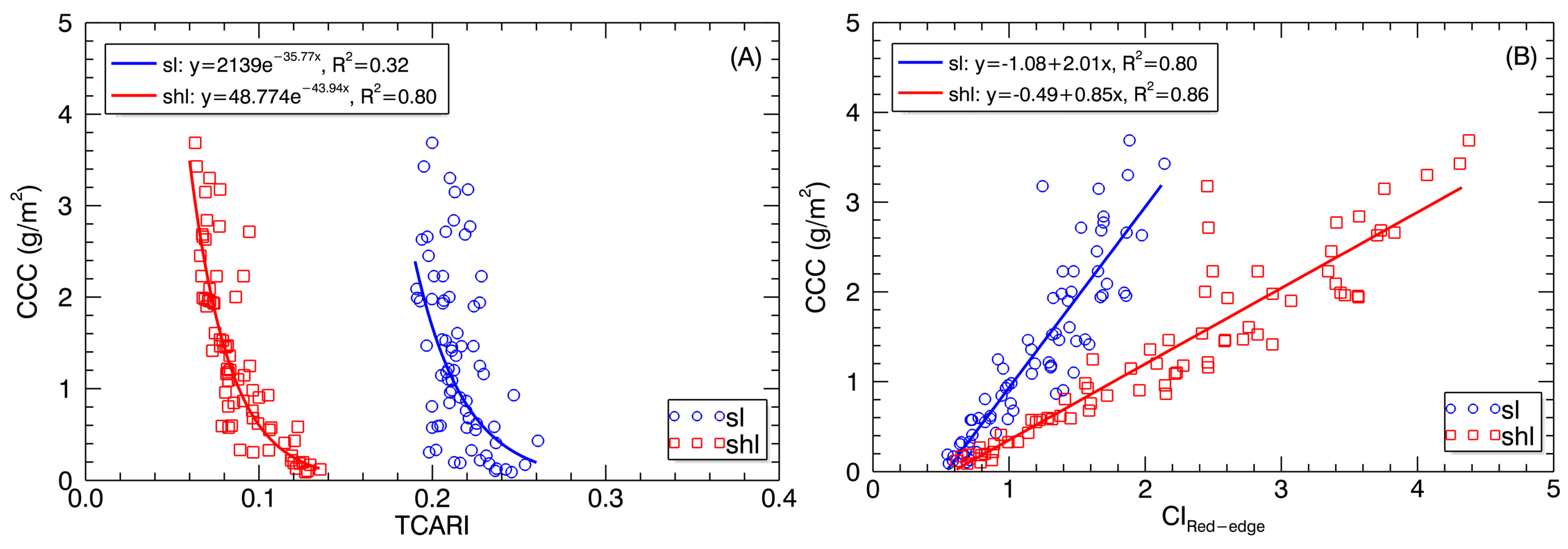
Figure 9.
Best-fit relationships of (A) TCARI and (B) CIRed-edge derived from SL and SHL pixels with CCC.
Figure 9.
Best-fit relationships of (A) TCARI and (B) CIRed-edge derived from SL and SHL pixels with CCC.
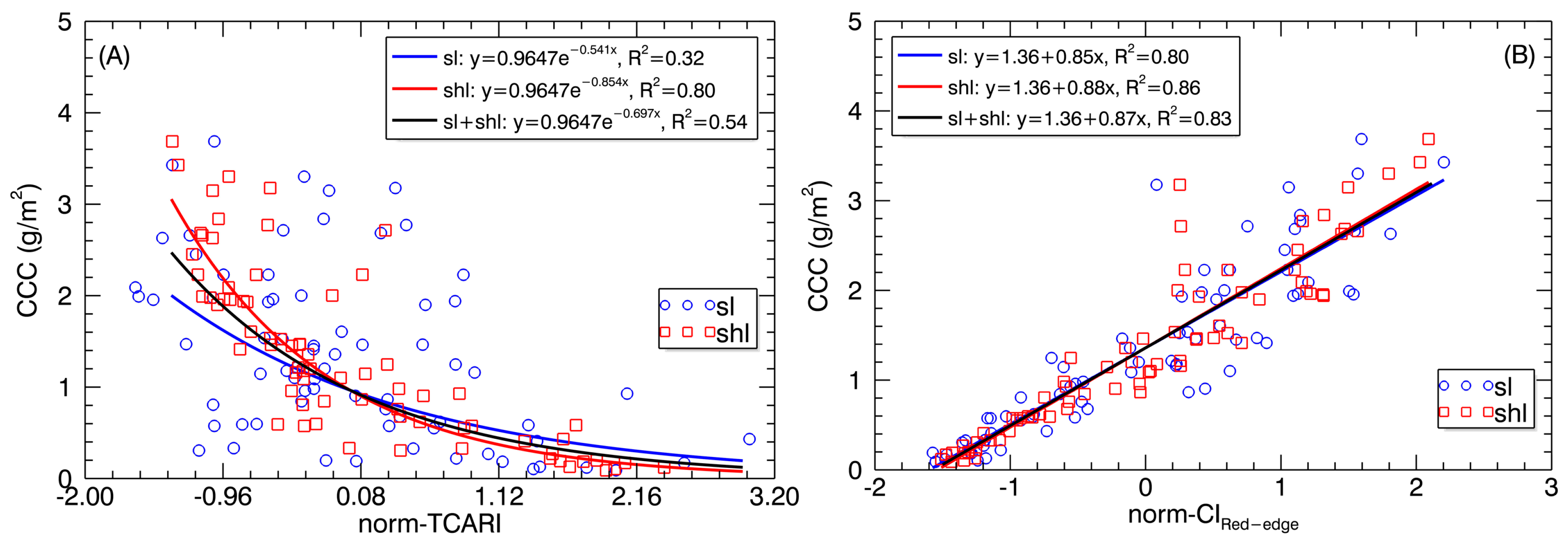
Figure 10.
Relationships of the (A) normalized TCARI (norm-TCARI) and (B) normalized CIRed-edge (norm-CIRed-edge) derived from SL and SHL pixels with canopy chlorophyll content.
Figure 10.
Relationships of the (A) normalized TCARI (norm-TCARI) and (B) normalized CIRed-edge (norm-CIRed-edge) derived from SL and SHL pixels with canopy chlorophyll content.
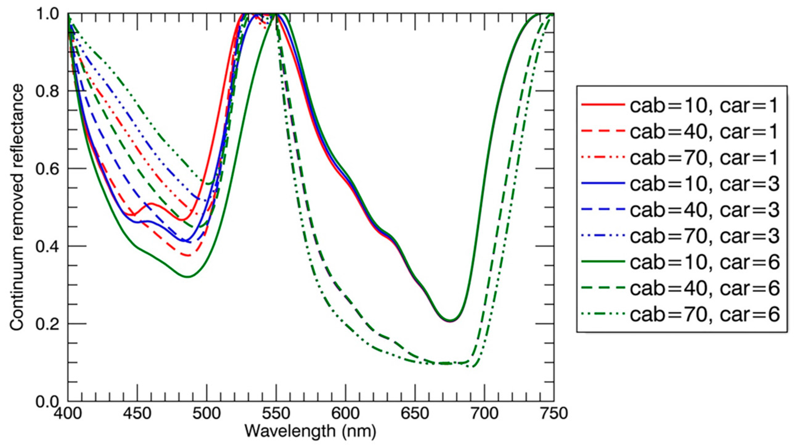
Figure 11.
The continuum removed reflectance spectra derived from the simulated reflectance spectra with the PROSAIL model. Fixed parameters for the PROSAIL model were: equivalent water thickness = 0.018 cm, dry matter content = 0.004 g/cm2, leaf structure parameter = 1.55, average leaf angle = 45°, LAI = 2.0, hot spot = 0.15, solar zenith angle = 30°, view zenith angle = 0°, relative azimuth angle = 0°, diffuse/direct radiation = 10. Varying parameters for the PROSAIL model were: chlorophyll content (Cab) = 10 μg/cm2, 40 μg/cm2, 70 μg/cm2; carotenoid content (Car, μg/cm2) = 1 μg/cm2, 3 μg/cm2, 6 μg/cm2.
Table 1.
Summary of image acquisition conditions for the rice experiment.
Table 1.
Summary of image acquisition conditions for the rice experiment.
| Date | Time (GMT+8) | Range of Solar Zenith Angle | Growth Stage |
|---|
| 8 July 2014 | 09:50–14:50 | 31.1°–37.9° | Early tillering |
| 20 July 2014 | 10:00–15:20 | 30.1°–44.7° | Fully tillering |
| 4 August 2014 | 10:05–15:20 | 30.9°–46.3° | Jointing |
| 20 August 2014 | 10:00–15:10 | 34.2°–47.1° | Booting |
| 3 September 2014 | 10:10–15:30 | 35.1°–54.8° | Heading |
| 20 September 2014 | 09:40–15:00 | 43.8°–54.0° | Filling |
Table 2.
Statistics of leaf and canopy chlorophyll content data for the experiment. Min: minimum value; Max: maximum value; Mean: mean value; SD: standard deviation; CV: coefficient of variation.
Table 2.
Statistics of leaf and canopy chlorophyll content data for the experiment. Min: minimum value; Max: maximum value; Mean: mean value; SD: standard deviation; CV: coefficient of variation.
| Chlorophyll Parameters | Min | Max | Mean | SD | CV (%) |
|---|
| Leaf chlorophyll content (LCC) (μg/cm2) | 30.51 | 48.80 | 41.94 | 4.94 | 11.77 |
| Canopy chlorophyll content (CCC) (g/m2) | 0.09 | 3.69 | 1.36 | 0.95 | 69.96 |
Table 3.
The averages of spectral angle mapper (SAM) values (unit: radians) for all spectra of each class (No. = 5760) as compared with mean reflectance spectrum/mean continuum-removed spectrum of individual classes.
Table 3.
The averages of spectral angle mapper (SAM) values (unit: radians) for all spectra of each class (No. = 5760) as compared with mean reflectance spectrum/mean continuum-removed spectrum of individual classes.
| Averages of SAM Values | Mean Spectrum of SL | Mean Spectrum of SHL | Mean Spectrum of SP | Mean Spectrum of SHP |
|---|
| SL | 0.07/0.08 | 0.15/0.15 | 0.11/0.20 | 0.11/0.16 |
| SHL | 0.14/0.18 | 0.08/0.12 | 0.20/0.31 | 0.10/0.21 |
| SP | 0.10/0.19 | 0.21/0.29 | 0.06/0.08 | 0.15/0.16 |
| SHP | 0.10/0.17 | 0.07/0.20 | 0.15/0.18 | 0.05/0.10 |
Table 4.
The averages of spectral information divergence (SID) values for all spectra of each class (No. = 5760) as compared with mean reflectance spectrum/mean continuum-removed spectrum of individual classes.
Table 4.
The averages of spectral information divergence (SID) values for all spectra of each class (No. = 5760) as compared with mean reflectance spectrum/mean continuum-removed spectrum of individual classes.
| Averages of SID Values | Mean Spectrum of SL | Mean Spectrum of SHL | Mean Spectrum of SP | Mean Spectrum of SHP |
|---|
| SL | 0.01/0.01 | 0.06/0.02 | 0.03/0.03 | 0.02/0.02 |
| SHL | 0.06/0.03 | 0.02/0.01 | 0.13/0.08 | 0.04/0.04 |
| SP | 0.03/0.03 | 0.13/0.07 | 0.00/0.01 | 0.04/0.02 |
| SHP | 0.01/0.02 | 0.03/0.04 | 0.04/0.02 | 0.01/0.01 |
Table 5.
Squared correlation coefficients (R2) from Spearman correlation for VIs derived from SL and SHL pixels in relation to LCC and CCC.
Table 5.
Squared correlation coefficients (R2) from Spearman correlation for VIs derived from SL and SHL pixels in relation to LCC and CCC.
| VIs | LCC | CCC |
|---|
| NDVI_sl | 0.45 ** | 0.63 ** |
| NDVI_shl | 0.58 ** | 0.81 ** |
| TCARI_sl | 0.26 ** | 0.25 ** |
| TCARI_shl | 0.62 ** | 0.75 ** |
| PRI_sl | 0.08 | 0.11 * |
| PRI_shl | 0.29 ** | 0.46 ** |
| CIRed-edge_sl | 0.54 ** | 0.84 ** |
| CIRed-edge_shl | 0.61 ** | 0.90 ** |
Table 6.
Coefficient of determination (R2) for the relationships between z-score normalized VIs derived from SL and SHL pixels and CCC.
Table 6.
Coefficient of determination (R2) for the relationships between z-score normalized VIs derived from SL and SHL pixels and CCC.
| VIs | SL | SHL | Combined |
|---|
| Linear Fit | Exponential Fit | Linear Fit | Exponential Fit | Linear Fit | Exponential Fit |
|---|
| NDVI | 0.55 | 0.63 | 0.62 | 0.87 | 0.58 | 0.75 |
| TCARI | 0.23 | 0.32 | 0.63 | 0.80 | 0.41 | 0.54 |
| PRI | 0.11 | 0.08 | 0.50 | 0.40 | 0.27 | 0.21 |
| CIRed-edge | 0.80 | 0.78 | 0.86 | 0.81 | 0.83 | 0.80 |


 ,
, 


