
On Multi-Hop Decode-and-Forward Cooperative Relaying for Industrial Wireless Sensor Networks

Faculty of Engineering, Norwegian University of Science and Technology (NTNU), N-2815 Gjøvik, Norway
*
Author to whom correspondence should be addressed.
Sensors 2017, 17(4), 695; https://doi.org/10.3390/s17040695
Submission received: 2 February 2017
/
Revised: 21 March 2017
/
Accepted: 26 March 2017
/
Published: 28 March 2017
(This article belongs to the Section Sensor Networks)
Abstract
:Wireless sensor networks (WSNs) will play a fundamental role in the realization of Internet of Things and Industry 4.0. Arising from the presence of spatially distributed sensor nodes in a sensor network, cooperative diversity can be achieved by using the sensor nodes between a given source-destination pair as intermediate relay stations. In this paper, we investigate the end-to-end average bit error rate (BER) and the channel capacity of a multi-hop relay network in the presence of impulsive noise modeled by the well-known Middleton’s class-A model. Specifically, we consider a multi-hop decode-and-forward (DF) relay network over Nakagami-m fading channel due to its generality, but also due to the absence of reported works in this area. Closed-form analytical expressions for the end-to-end average BER and the statistical properties of the end-to-end channel capacity are obtained. The impacts of the channel parameters on these performance quantities are evaluated and discussed.
1. Introduction
In recent years, technological concepts such as Industry 4.0, smart home, and smart grid are set to reshape the landscape of future industry and people’s lifestyle more than we ever thought possible. The common vision of such systems is generally connected to one single concept, the Internet of Things (IoT), where through the use of wireless sensor networks (WSNs), the entire physical infrastructure is closely coupled with the achievement of intelligent monitoring and management [1,2]. WSNs can provide great operating effectiveness through low installation and operating costs, installation flexibility, and scalability. They have be used in a broad range of scenarios such as smart home services [3], disaster detection and relief [4], and industrial automation [5,6].
A sensor network typically consists of a number of inexpensive low-power sensor nodes, which are distributed across a large area and can perform the tasks of data sensing, simple information processing, and communication over short distances [7]. Arising from the presence of spatially distributed sensor nodes in a sensor network, cooperative diversity can be achieved by using the sensor nodes between a given source-destination pair as intermediate relay stations. This kind of communication scheme provides significant robustness against the adverse effects of shadowing and fading in wireless communications, which leads to broader coverage, enhanced mobility, and improved system performance compared to the direct transmission [8,9,10]. Depending on the nature and complexity of the relaying technique, the relaying strategies can be generally classified into two categories, namely decode-and-forward (DF) and amplify-and-forward (AF) [11,12,13].
The performance analysis of DF and AF relaying systems under different channel conditions has been the topic of a wealth of papers. In the most recent work, the analytical expressions of the end-to-end average bit error rate (BER) for DF relaying systems over Rayleigh and Nakagami-m fading channels with additive white Gaussian noise (AWGN) have been derived in [14,15], respectively. The ergodic capacities of the DF relaying systems in Rayleigh, Rician, and Nakagami-m fading channels have been analyzed in [16,17,18], respectively. However, the analyses are made for the particular case of only two consecutive hops, which limits the use of the results. The ergodic capacity for multi-hop AF relaying systems over Rayleigh fading channels was investigated in [19]. In [20], the authors derived a tight lower bound for the error rate and the outage probability of cooperative diversity networks over independent non-identical Nakagami-m fading channels with AF relaying and maximum ratio combining (MRC) at the destination node. In [21], an upper bound for the ergodic capacity of multi-hop cooperative relaying channels over independent non-identically distributed (i.n.i.d.) Nakagami-m fading was derived assuming AF relays. From the aforementioned up-to-date reported works, it is fairly evident that the ergodic capacity for multi-hop DF relaying systems over Nakagami-m fading channels is not explored from the analytical point of view.
Meanwhile, the vast majority of the analyses on the performance of wireless communication systems in the open literature have been based on the assumption of interference amplitude following Gaussian distribution with flat power spectral density (i.e., AWGN) owing to its simplicity for analysis. However, the AWGN channel model does not cover the behavior of a large class of commonly occurring interference signals such as electromagnetic interference and man-made noises, which cannot be ignored in many scenarios ([22], pp. 84–90). For example, in harsh industrial environments where WSNs will play a vital role in the Industry 4.0 era, the effects of noise and interferences are significant due to the wide operating temperatures, strong vibrations and excessive electromagnetic noise caused by large motors and other equipment [23,24,25]. Therefore, the impulsive noise should be taken into consideration while analyzing the performance of WSNs for industrial applications. To this regard, a more practical model is the Middleton’s Class-A (MCA) model, which has shown to provide excellent fits to a variety of noise and interference measurements [26,27,28]. The advantage of this model lies in its generality to represent a number of interference signals with arbitrary impulsive effects. By varying model parameters, we can model a wide class of interferences ranging from pure AWGN to highly impulsive noise [29,30].
In light of this, we present the performance analysis of multi-hop DF relaying system over Nakagami-m fading channels in the presence of impulsive noise. The justification for the choice of Nakagami-m distribution as the small-scale fading in our analysis is threefold. Firstly, a large number of field measurements show that the small-scale fading in indoor environments follows Nakagami-m fading [31,32,33]. Secondly, Nakagami-m distribution describes via the m parameter a wide range of fading distributions. For instance, it converges to one-sided Gaussian distribution with , to Rayleigh with , and to purely Gaussian as m approaches infinity. Given appropriate bounds on the parameters, the lognormal and Weibull distributions can also be well approximated by the Nakagami-m distribution in some ranges ([34], pp. 284–288). Furthermore, it can also closely approximate the Nakagami-n (Rice) and Nakagami-q (Hoyt) distributions with appropriate parameter mappings ([35], p. 25). Thus, our results can be readily extended to other fading scenarios by simply varying the model parameters. Last but not least, to the best of our knowledge, it is still an open research question on the capacity performance of multi-hop DF relaying systems over Nakagami-m fading channels. In this paper, we intend to fill this gap.
The remainder of this paper is organized as follows. In Section 2, we introduce the cooperative transmission system under investigation as well as the fading channel and noise model. In Section 3, closed-form expressions for the end-to-end average BER of the relaying system under the considered channel condition are derived. The analytical expression for the end-to-end average capacity and the statistics of the end-to-end instantaneous capacity are derived in Section 4. Analytical and simulation results are presented and discussed in Section 5. Section 6 concludes the paper and discusses about future work.
2. System and Channel Model
2.1. Notation
A number of notations are used throughout the paper, here we highlight the following notations and their corresponding meanings: denotes the probability density function (PDF) of the random variable (RV) x; represents the cumulative distribution function (CDF) of the RV x. The symbols and are the transmitted power and the received signal power by node , respectively. The RV represents the noise of the ℓ-th link modelled by MCA model. The symobl represents the average BER of the ℓ-th hop transmission; and denotes the average BER after the ℓ-th transmission compared with the bits transmitted by source node .
2.2. System Model
In our work, we consider a multi-hop wireless relay system with L hops using DF relaying strategy. Figure 1 illustrates the investigated scenario, where the nodes and correspond to the source node and destination node, respectively; and the link between the nodes and , , is denoted as ℓ-th hop with separation distance . Full-duplex mode of communication is assumed, in which the nodes can transmit and receive at the same time employing frequency division duplexing (FDD). In FDD mode, each node use frequency bands and to transmit and receive data, respectively. Altogether, there are L such non-overlapping frequency pairs; and only a subsequent node can listen to the signal transmitted by a previous node, thus avoiding the interference in any hop owing to the transmissions occurring in the surrounding hops. The channels between adjacent nodes and , , are mutually independent and undergo Nakagami-m fading.
Data transmission is done using the M-ary phase shift keying (M-PSK) symbols with equal a priori probabilities. The node , , transmits the unit-energy M-PSK symbol (i.e., ) with power . The corresponding received signal at node and the total transmit power of the relay system can be written as
where is the received signal power by node ; and are the channel fading amplitude and the additive noise of the ℓ-th hop, respectively. The received signal power by node depends on the transmitted signal power by the previous node and the distance between the two nodes. A widely used model for the signal attenuation is the one-slope path-loss model [33]. According to the one-slope model, the relationship between and can be expressed as
where is the path-loss exponent, which reflects the rate at which the received power decreases with distance. The value of the parameter in a specific environment could be simply obtained by field measurement [36,37,38] or estimated using numerical algorithms [39,40]. The overall performance of the DF relaying network is limited by the worst link, it is thus straightforward to show that in order to obtain the best performance, the total power should be allocated among different hops in a way such that the received signal power is equal for each receiving node, i.e., , . From (3), this constraint of the received powers translates into the following relationship on the transmitted power of each node
2.3. Channel Model
The channel fading amplitudes () in (1) are modelled as independent and identically distributed (i.i.d.) Nakagami-m RVs. The PDF of the RVs () is expressed as
where represents the complete Gamma function defined as , is the expectation of ; and m is the Nakagami-m fading parameter, which determines the severity of fading channels and ranges from 0.5 to ∞.
The additive noise () in (1) are i.i.d. RVs modeled by the MCA model. The PDF of the RVs is given by [41]
where denotes a zero-mean Gaussian PDF with variance ; and the parameter is the Poisson-distributed probability expressed by
The variance in (6) and (7) is defined with the auxiliary RV as follows:
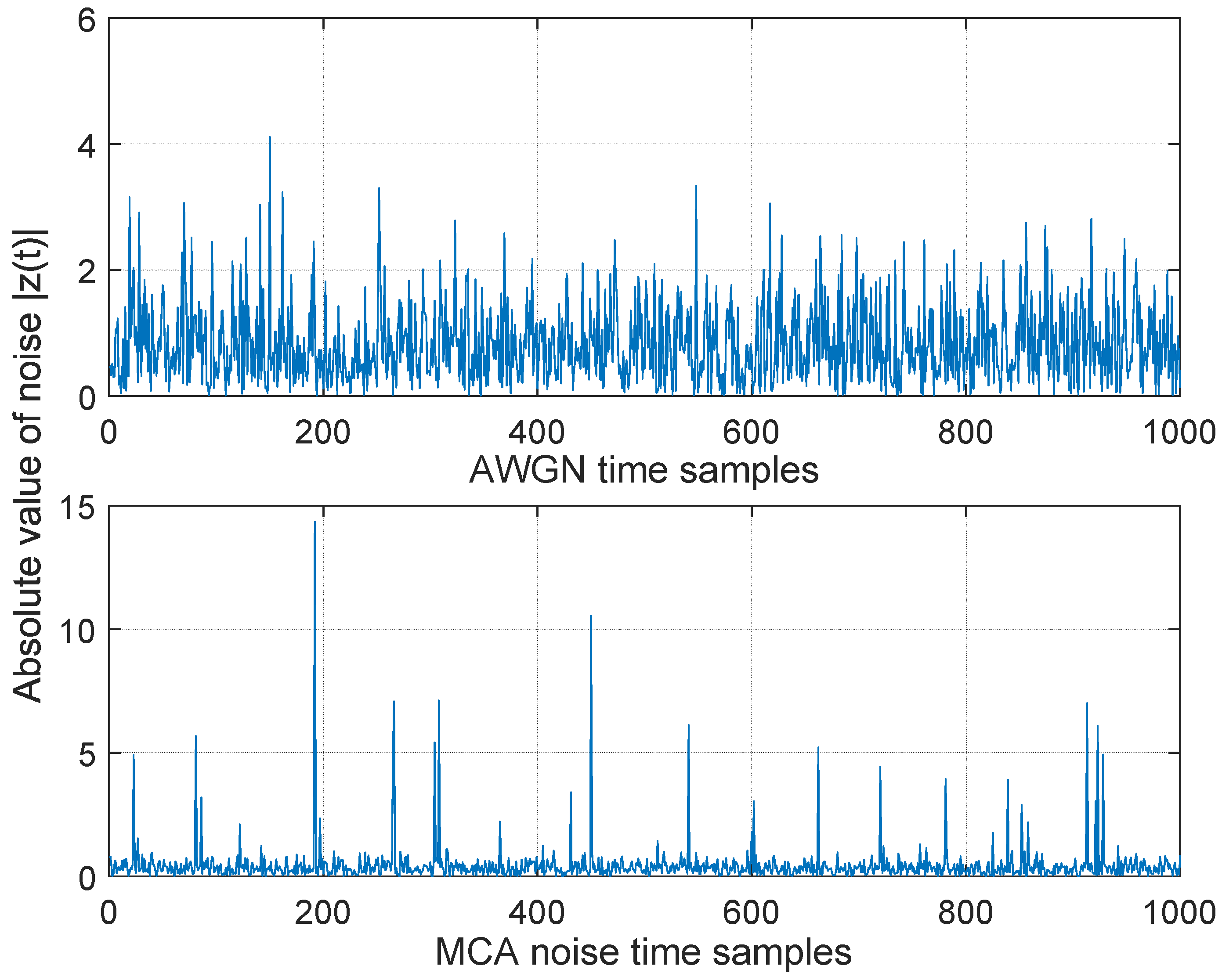
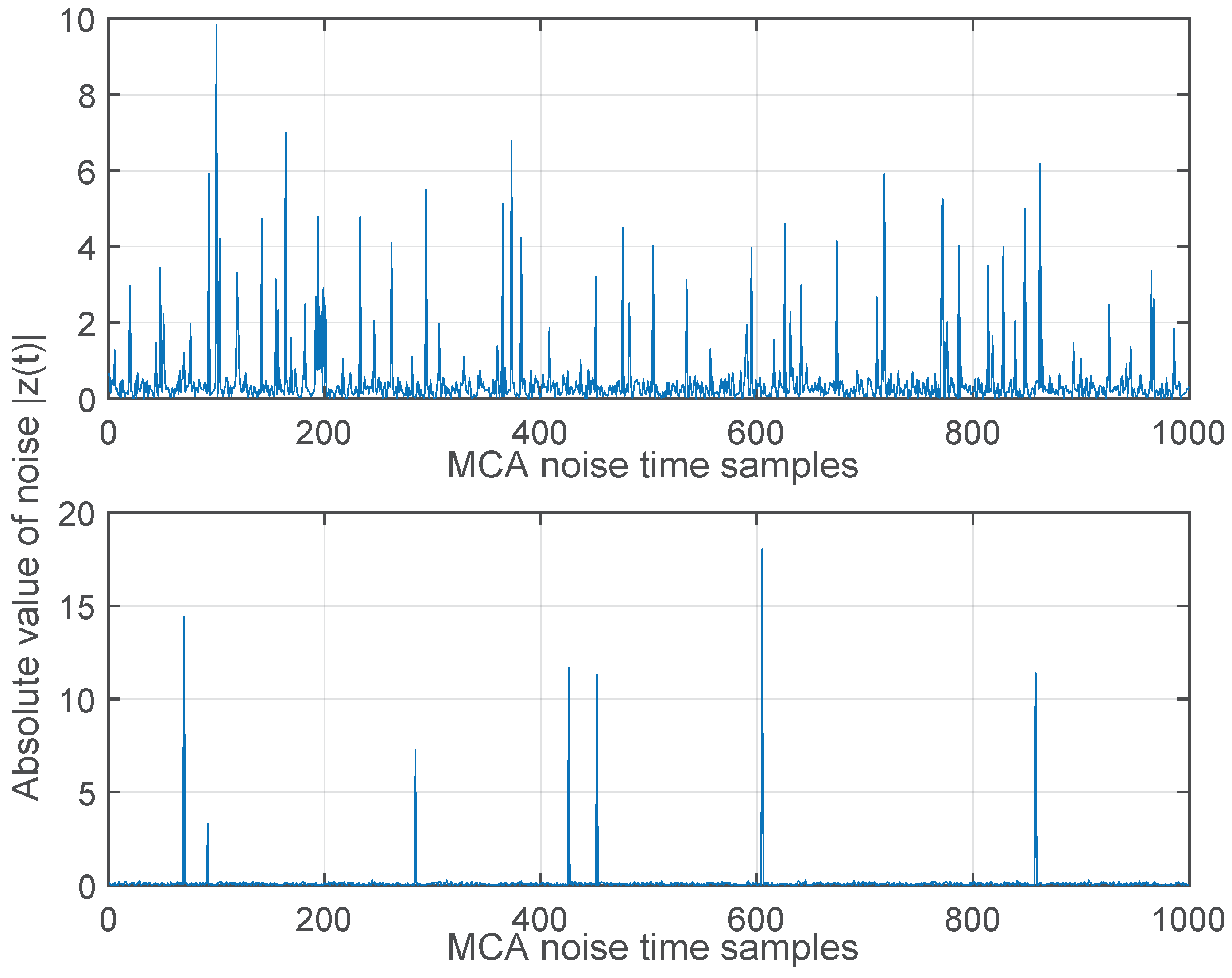
where represents the ratio of the Gaussian noise power to the impulsive noise power . The parameter A is called the impulsive index and defined as the product of average rate of impulsive noise and mean duration of the impulsive interference. The impulsive index determines impulsiveness the noise: a smaller value of the impulsive index implies a higher level of impulsive interference. It is known that as A approaches a value around 10 or larger, the MCA distribution is very close to a Gaussian PDF; while for A and lower than 1, the PDF gets very heavy tails and the interference can be seen as very impulsive [26]. The extraction of MCA model parameters from real measurements can be done with the algorithms developed in (e.g., [42,43]). It should be noted that the MCA model includes both the impact of impulsive interference as well as thermal noise in the communication systems [41]. Figure 2 shows the difference between pure AWGN and impulsive noise generated with the MCA model and Figure 3 illustrates the effects of the parameters A and used in the MCA model.
As can be seen from (7), the MCA model can be interpreted as a Gaussian-mixture model [44]. Therefore, it is straightforward to show that the mean of the noise ; and the average power of the noise, i.e., the variance of , is calculated as
Alternatively, the generation of MCA noise can be interpreted as a stationary random process: for each channel realization, the probability of experiencing an interference noise with distribution is given in (8). Despite the PDF in (7) has an infinite number of terms, we can safely restrict our analysis to the first N terms without significant loss by noticing that as n increases, the probability approaches zero and is thus negligible. The number N can be obtained from
where is an arbitrary positive number.
3. Bit Error Rate Performance Analysis
3.1. The Instantaneous SNR
To derive the BER and channel capacity of the relaying system, we first derive the statistics of the signal-to-noise ratio (SNR). Let be the instantaneous SNR pertaining to the ℓ-hop transmission, which is given by
3.2. The End-to-End Average BER
Proposition 1.
The average BER of the M-ary phase shift keying (M-PSK) for the ℓ-th hop over the Nakagami-m fading channel in the presence of impulsive noise is given by
where , and 2 represents the Gauss hypergeometric function ([46], p. 1005) defined by
with denoting the ascending factorial.
Proof.
See Appendix A.1. ☐
Remark.
The average BER of equiprobable binary phase shift keying (BPSK) modulated symbols for the ℓ-th hop over the Nakagami-m fading channel in the presence of impulsive noise can be readily obtained from (18) as follows:
Proposition 2.
If the average BER per hop is the same for all hops (namely, , ), then the end-to-end average BER of L-hop the wireless DF relaying system can be expressed as:
Proof.
See Appendix A.2. ☐
Figure 4 shows the relationship between the end-to-end average BER of the L-hop relay system and the single-hop average BER in log-log representation assuming the identical statistical behavior for all single hops. From Figure 4, we can observe a nearly linear relationship between the two BERs when the single-hop average BER is below some threshold. This linearity can be theoretically proved by noticing that the linear term will dominate for low values of after extending the power series in (21) ([46], p. 25).
4. Channel Capacity Performance Analysis
By comprehending the MCA noise channel as a Gaussian-mixture channel in (7), the instantaneous channel capacity per unit bandwidth of the ℓ-th link can be obtained according to the theorem of total probability ([45], p. 23), i.e.,
where and are given in (8) and (10), respectively.
According to the well-known max-flow min-cut theorem, the maximum achievable channel capacity of a multi-hop relay system from the source node to the destination node is bounded by the minimum of the capacities of each individual hop ([47], pp. 587–595). Therefore, the instantaneous channel capacity of the end-to-end full-duplex relay network can be written as
where is the effective SNR equivalent to one-hop transmission channel with the same capacity as the L-hop DF relay channel.
Proposition 3.
The PDF of the equivalent SNR of the L-hop relay system is expressed as
Proof.
4.1. The End-to-End Average Capacity
The end-to-end average channel capacity of the relay network can be obtained from
where is the instantaneous capacity in (23) and is the PDF of the equivalent SNR given in (24). The closed-form expression for the average capacity is given below.
Proposition 4.
The end-to-end average capacity of the L-hop relay network under the balanced power allocation scheme can be expressed as follows:
where the k-th moments of can be expressed as follows
with , , , and are computed recursively with .
Proof.
See Appendix B.1. ☐
4.2. Statistics of the End-to-End Instantaneous Capacity
The expression of the end-to-end instantaneous capacity of the multi-hop relay network is given in (23). To obtain the statistics of , we define an auxiliary variable called partial channel capacity as follows:
where N is calculated from (13). With the assumptions in Section 2, it is straightforward to show that the auxiliary variables are mutually independent.
Next, by applying the concept of transformation of random variables on (30) ([45], pp. 100–108), the PDF of the variable can be obtained from
where the function is expressed in (24), and are given in (8) and (10), respectively.
Finally, it is known that the PDF of the sum of multiple independent random variables, each of which has a PDF, is the convolution of their separate density functions ([45], pp. 182–186). Therefore, from (31), the PDF of the end-to-end instantaneous channel capacity C is expressed as
where ∗ denotes the convolution operator, and the expression of the PDFs is given in (32) and (13). There exists no closed-form solution to the convolution in (33), but it can be numerically evaluated using mathematical softwares such as Mathematica and Matlab.
The variance of the channel capacity is a measurement of the spread of the instantaneous capacity around the average capacity. The variance of the end-to-end instantaneous capacity, denoted as , is defined as
where is the end-to-end average capacity given in (A9), and is the PDF of the end-to-end instantaneous capacity expressed in (33). Closed-form analytical expression for the variance of the channel capacity given in (34) is very difficult to obtain. Nevertheless, the result can be obtained numerically, as will be presented in Section 5.2.
5. Numerical Results
In this section, we will present and discuss the analytical results obtained in the previous sections. The validity of the theoretical results is confirmed with Monte Carlo simulations.
5.1. Results on Average BER
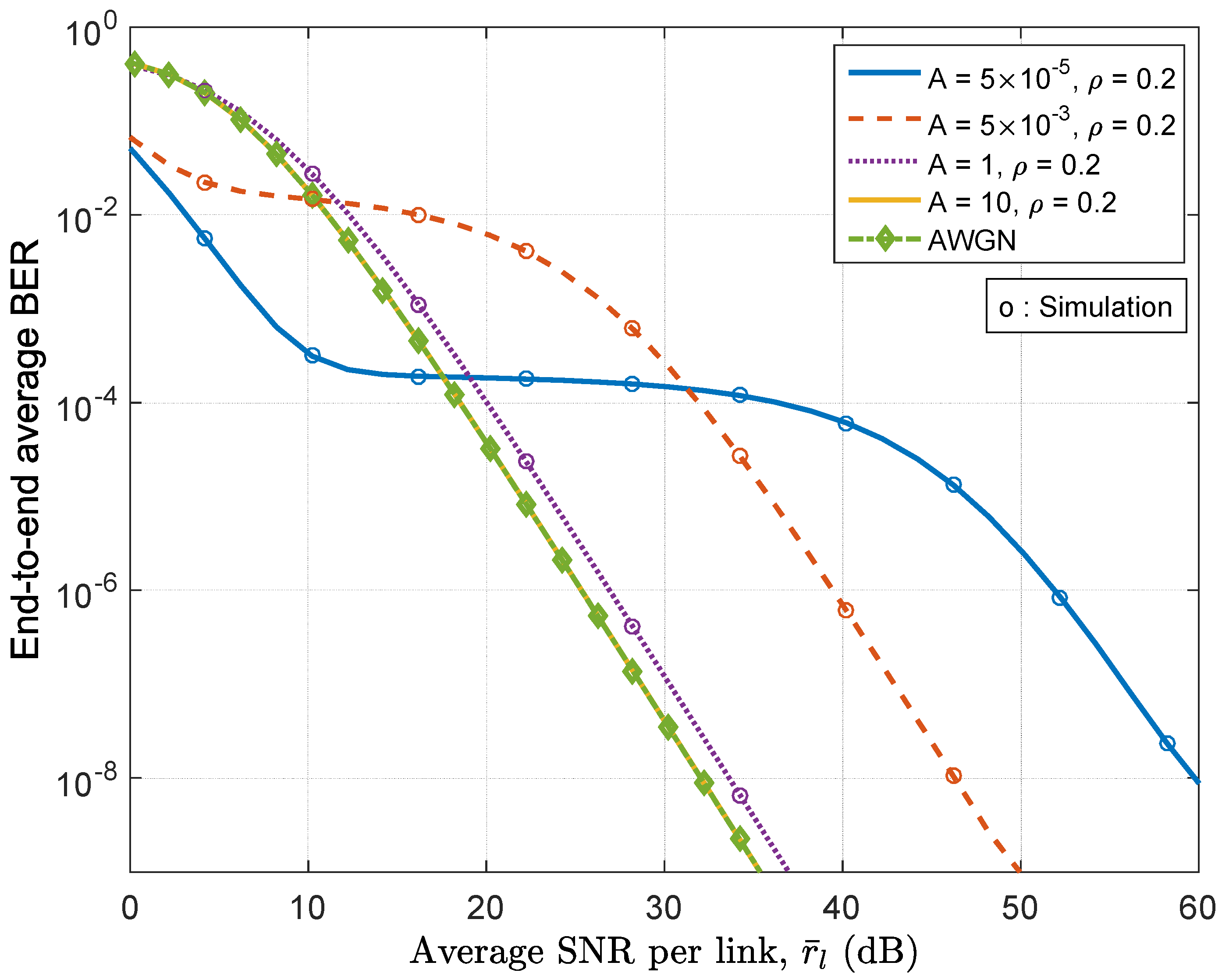
In Figure 5, we present the end-to-end average BER for BPSK modulation signals of an 8-hop relay system against the average SNR of each hop over Nakagami-m fading channels with in the presence of impulsive noise with various levels of impulsiveness (i.e., from highly impulsive with , moderately impulsive with to rarely impulsive with , the ratio is fixed as ). The theoretical curves are obtained using the closed-form expressions given by (A5) and (18) and are found to agree well with the simulation results, thus validating our analysis. It can be seen that when the parameter A is equal to 10, the corresponding curve is extremely close to the result obtained under AWGN assumption, which is in accordance with our statement that when A is equal to or greater than 10, the MCA channel degenerates to an AWGN channel. It can also be observed from Figure 5 that the performance under impulsive noise is dramatically different from that under the AWGN. Under a highly impulsive noise condition, a three-region performance behavior is observed: the BER curve first decreases almost linearly with increasing SNR, and then remains almost stagnant for some SNR region until finally decreases again after increasing the SNR to a larger value. This phenomenon can be best explained by the envelop distribution analyses of the MCA interferences in [43]. It has been observed that the distributions of the noise envelop z are divided into three parts, the first corresponds to smaller values of z, in which the Gaussian noise component dominates; the second corresponds to larger values of z, wherein the impulsive noise component dominates; and the third corresponds to intermediate values of z, for which the CDF is virtually constant for these values. The portion of the distribution corresponding to these intermediate values of z is termed the “null region” [43]. Therefore, we can conclude that the first decrease in the BER plot is mainly affected by the Gaussian noise component with small envelopes; and the second decrease is mainly determined by the impulsive noise component while the stagnant flat-region in the BER plot is due to the existence of the “null region” in the envelope distribution of the MCA noise.
An advantage of our analysis lies in its flexibility for the performance evaluation under various channel conditions. For illustration purposes, Figure 6 shows the BER results of the Rayleigh fading channels in various noise conditions and the purely AWGN channel by setting the appropriate Nakagami-m and MCA parameters.
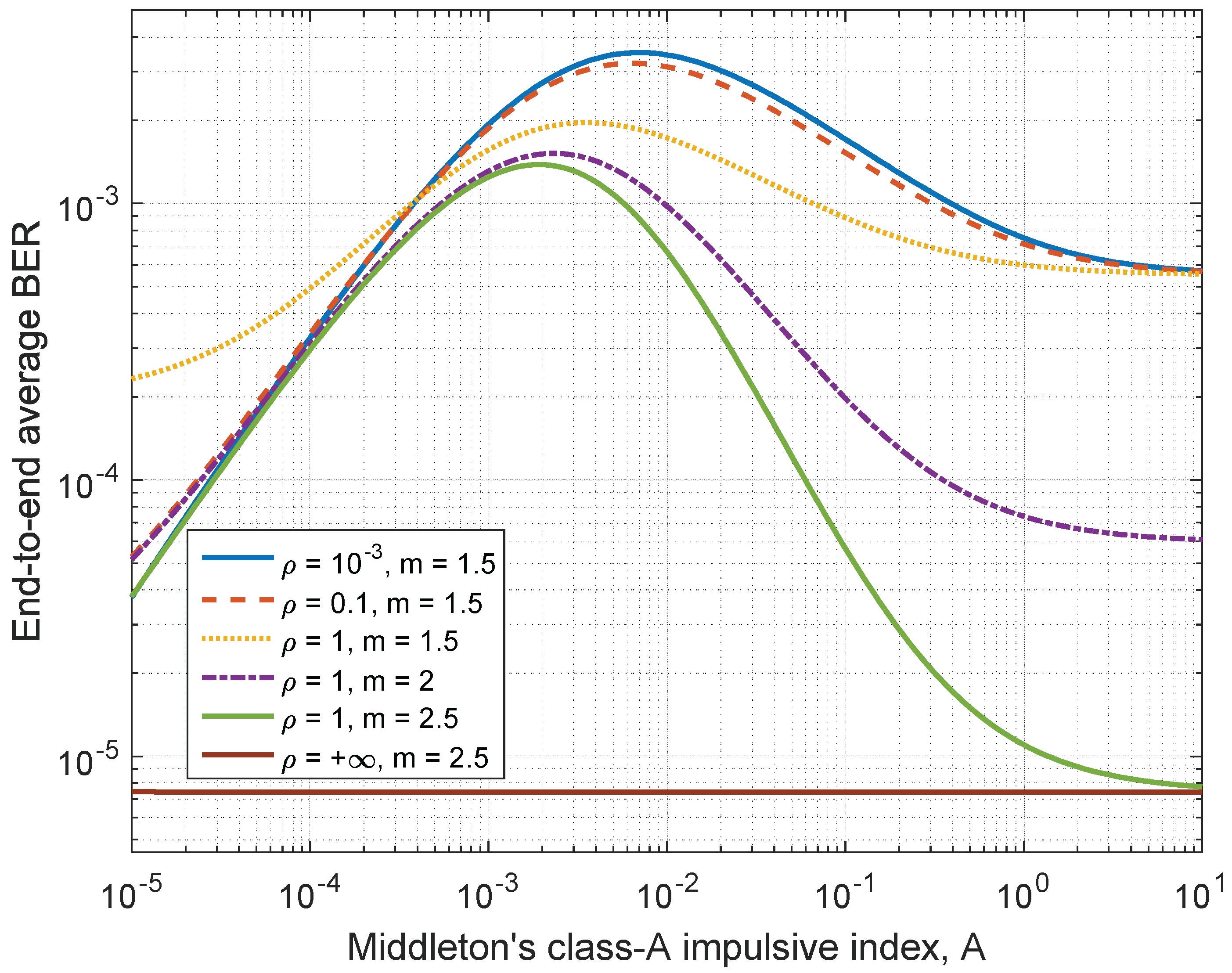
The effects of the impulsive index A and the ratio on the end-to-end BER performance of the multi-hop relay network are investigated in Figure 7. It shows the average BER under various values of A and for an 8-hop relay network with average SNR being 25 dB. It is observed that the BER is not a monotonic function of the impulsive index A with fixed values of . When the channel noise changes from highly impulsive to approximately Gaussian , the BER first increases for some range of A before reaching a peak point; then with further increase of A to around 10, the BER gradually decrease to the value under AWGN channel. The value of corresponds to the case of purely AWGN channel, thus the BER value does not depend on A in this case and is always equal to the value of AWGN case.
In Figure 8, we present the end-to-end average BER performance of a relay network against total power consumption under two different power allocation schemes, i.e., the scheme of equal power allocation among all transmitting nodes, and the scheme of balanced power allocation taken into consideration the path loss of each hop. The following parameters are used for the simulation: , , , ; and the distances of each hop is set as meters. The BER results under the equal power allocation scheme are calculated recursively using (A4). It can be seen that the performance under balanced power allocation scheme is generally better than that under the equal power allocation scheme. Also, the performance difference between the two schemes becomes larger when the path loss exponent is greater. This is because under the balanced power allocation scheme, the performances of all hops are always identical; while for the equal power allocation scheme, when the path loss exponent is larger, the variance of the performances of each hop also becomes larger. This eventually leads to poorer performance of the relaying system since the end-to-end performance of the DF relaying network is dominated by the performance of the worst hop.
5.2. Results on Channel Capacity
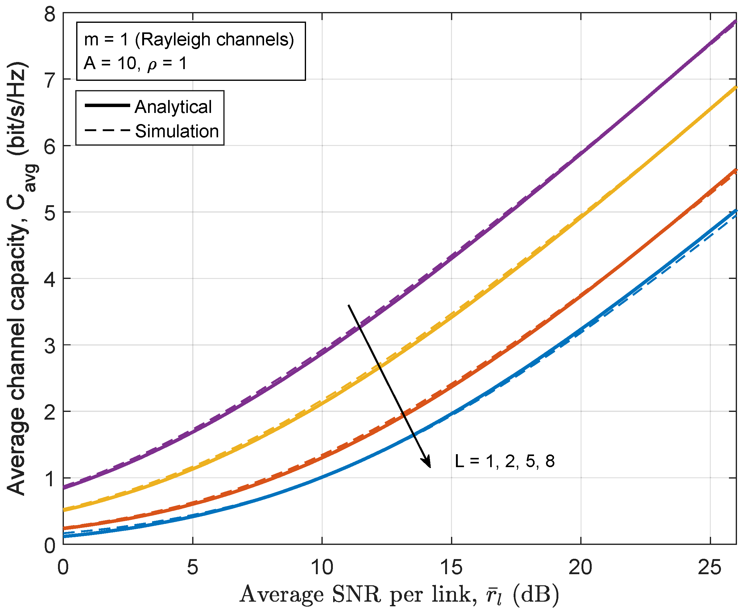
Figure 9 and Figure 10 sketch the end-to-end average capacity of the relay network employing the full-duplex communication mode and balanced power allocation scheme as a function of the average SNR for varying numbers of hops L. It can be seen that excellent fit is found between the analytical results from the proposed closed-form expression and the simulation results. Figure 9 shows the channel capacity of relay network under the Nakagami-m fading channels in the presence of mediumly impulsive noise with and . Figure 10 shows the channel capacity of the relay network under Rayleigh fading channels in the presence of nearly Gaussian noise with . As expected, the overall channel capacity degrades as L increases in exchange for broader transmission coverage. A less impulsive channel (i.e., when A or are large enough such that the MCA channel degenerates to the AWGN channel) gives a capacity approaching that of the AWGN channel. Since AWGN is known to be the worst additive interference in terms of channel capacity for both point-to-point channels and relay channels, all values of the different MCA model parameter sets provide higher capacity than the corresponding AWGN channel [48]. However, it should be noted that the AWGN channel does not necessarily underperform the corresponding MCA channel in terms of BER, as can be seen from Figure 7.
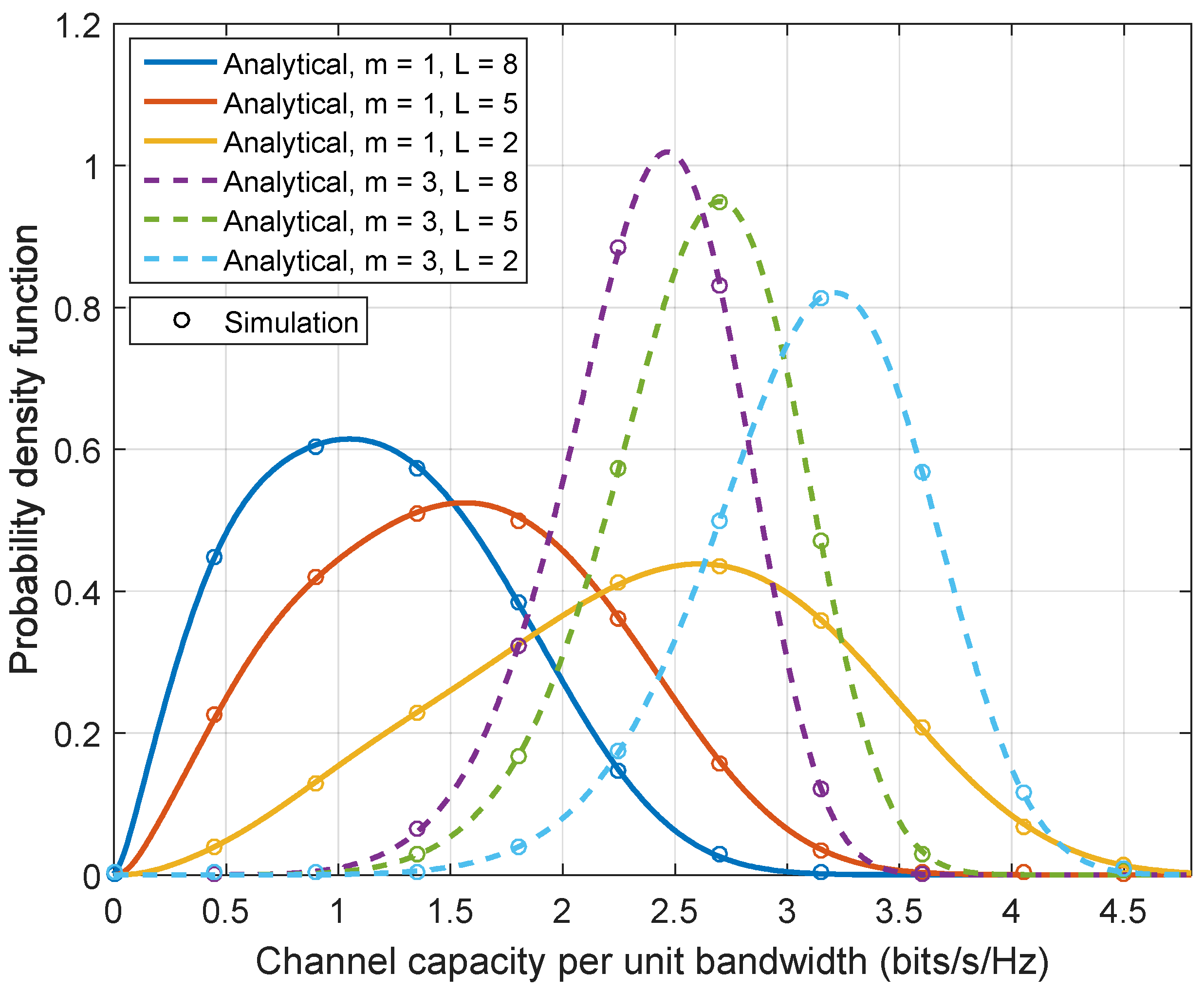
The PDFs of the end-to-end instantaneous capacity of the multi-hop relay system under Rayleigh and Nakagami-m fading channels are presented in Figure 11. The following parameters are considered: the impulsive index , the ratio , and the average SNR being 10 dB. It can be found from Figure 11 that an increase of the severity of large-scale fading (i.e., decreasing the value of the Nakagami-m parameter m) decreases the mean value of the channel capacity. Similarly, an increase of the number of hops L also degrades the mean channel capacity. These can also be evidenced by comparing Figure 9 and Figure 10. It can also be observed that a decrease in the parameter m or the number of hops L results in an increase of the variance of the channel capacity, which will be reconfirmed in Figure 12.
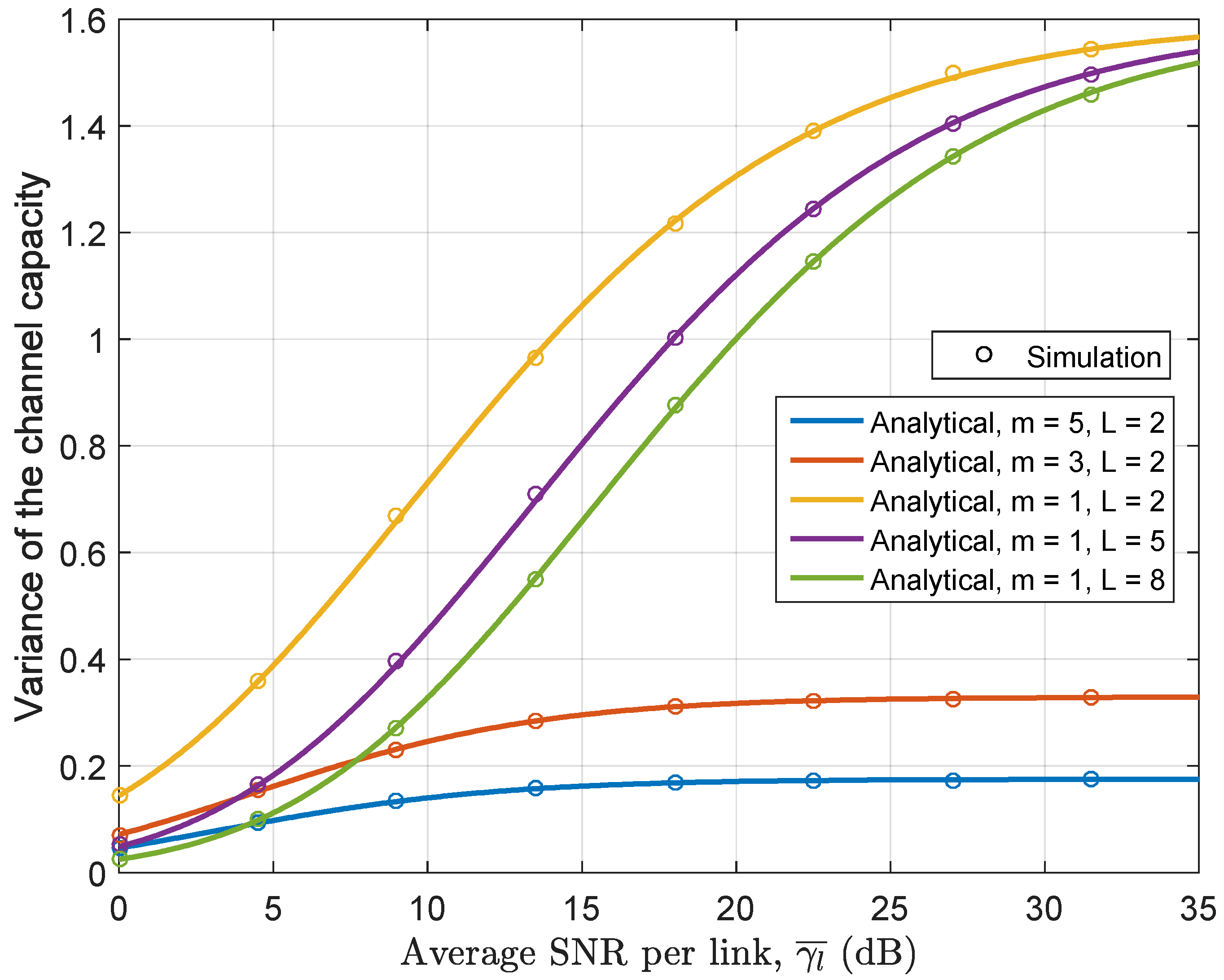
Figure 12 illustrates the behavior of the variance of the channel capacity with varying average SNR per link. We calculate the variance for different number of hops and varying values of the Nakagami m parameter. It is shown that the variance increases as the average SNR increases. More specifically, it is found that the variance increase monotonically from low SNR to high SNR region and afterward it continues to maintain approximately the same level in the high SNR region. The variation of the channel capacity is also found to increase with the reduction of the Nakagami m parameter or increase of the number of relay hops.
6. Conclusions
In this paper, we investigated the end-to-end average BER performance and the channel capacity of a multi-hop DF relay system over Nakagami-m fading in the presence of impulsive noise. The analysis were validated by showing the excellent agreement between the results obtained through the closed-form expressions and the Monte Carlo simulation results. The analysis is very general and can be easily extended to other channel conditions (e.g., the conventional Rayleigh fading over AWGN, etc.) by changing the parameters of the fading and the noise models. The impacts of the path loss exponent and the fading severity on the system performance are also investigated. It is shown that the increase of the number of hops will degrade both the BER and channel capacity but also decrease the variance of the channel capacity. In channel conditions with highly “impulsive” noise effects, the BER curve will experience a stagnant stage against the increase of the SNR due to the characteristics of the noise. As the path loss exponent of the propagation environment increases, the advantage of the balanced power allocation scheme becomes more obvious compared to the equal power allocation scheme with respect to the end-to-end BER.
Future work includes improvement of system performance under impulsive noise conditions by noticing that the existence of impulsive noise significantly degrades the performance, especially in the “null region”. This can be potentially achieved by predicting the occurrence of impulsive noise if possible and adjust the power or coding rate accordingly.
Acknowledgments
We gratefully acknowledge the Regional Research Fund of Norway (RFF) for supporting our research.
Author Contributions
Yun Ai proposed the research idea, performed the mathematical analysis and wrote the manuscript. Michael Cheffena supported and supervised the research as well as proofread the manuscript.
Conflicts of Interest
The authors declare no conflict of interest.
Appendix A. Bit Error Rate Performance Analysis
Appendix A.1. Derivation for the Average BER Pℓ in Proposition 1
Let be the conditional BER of the ℓ-th hop conditioned on SNR . By interpreting the MCA channel as a Gaussian-mixture model, the BER for M-ary PSK signals as a function of the SNR can be expressed as [49]
where , , is given in (8) and is the Gaussian Q-function.
The average BER of the ℓ-th hop over Nakagami-m fading in the presence of impulsive noise is given by
The indefinite integral in above expression is in the form of , which has the following solution [50]:
where 2 is the Gauss hypergeometric function.
Appendix A.2. Derivation for the BER Relationship in Proposition 2
In the investigated DF relay network, the transmitted information-bearing signal can be correctly decoded at the destination node if the relay performs correct detection, or if a relay makes an erroneous detection, which is rectified by further erroneous detection at subsequent relays [15]. Let denotes the BER after the ℓ-th hop transmission starting from the source node. Then, the end-to-end average BER for the wireless relay system can be written as
where is the average BER of the L-th hop transmission and can be calculated from (18).
If the channel conditions are identical for all hops and transmission power of each hop fulfils the constraint in (4), the average BER of all individual hops are equal (denoted as ). Then, we can extend the expression (A4) recursively and obtain the following relationship between the end-to-end average BER and the average BER of individual hops:
where the last equality is obtained based on the properties of geometric progression ([46], p. 1).
Appendix B. Channel Capacity Performance Analysis
Appendix B.1. Derivation of the Average Capacity in Proposition 4
To derive the closed-form expression for average capacity, we first obtain the following alternative expression of the logarithm term in (23) by expanding it to Taylor series ([51], p. 68):
Substituting (A7) and (23) into (27), we can obtain the following expression for the end-to-end average capacity of the multi-hop network:
It is obvious from (A9) that to calculate the average capacity, we need to derive the moments of the ratio . By definition, the k-th moment is formulated as
where the integral is given as
To obtain the closed-form expression for integral in (A10), we follow the similar rationale in [52], namely, representing the Gamma function as a sum of terms. The normalized upper incomplete Gamma function can be rewritten as an finite sum of terms ([46], p. 899), i.e.,
Next, we define and . According to the polynomial theory, the finite series in (A12) corresponds to a polynomial in with degree and coefficient ([46], p. 17). Then, the -th power of is equivalent to another polynomial with degree as follows
where the coefficients are expressed as
and
are computed recursively with .
Using (A12) and (A13) for the integral in (A10) and applying the equality [46, Eq. 3.384.3], we can obtain the exact closed-form solution for the integral as
References
- Sun, Y.; Lanctot, P.; Fan, J. White Paper: Internet of things: Wireless sensor networks; International Electrotechnical Commission: Geneva, Switzerland, 2014. [Google Scholar]
- Eugster, P.; Sundaram, V.; Zhang, X. Debugging the Internet of Things: The case of wireless sensor networks. IEEE Softw. 2015, 32, 38–49. [Google Scholar] [CrossRef]
- Byun, J.; Jeon, B.; Noh, J.; Kim, Y.; Park, S. An intelligent self-adjusting sensor for smart home services based on ZigBee communications. IEEE Trans. Consum. Electron. 2012, 58, 794–802. [Google Scholar] [CrossRef]
- Chraim, F.; Erol, Y.; Pister, K. Wireless Gas Leak Detection and Localization. IEEE Trans. Ind. Electron. 2015, 12, 768–779. [Google Scholar] [CrossRef]
- Das, K.; Zand, P.; Havinga, P. Industrial Wireless Monitoring with Energy-Harvesting Devices. IEEE Internet Comput. 2017, 21, 12–20. [Google Scholar] [CrossRef]
- Gungor, V.C.; Hancke, G.P. Industrial wireless sensor networks: Challenges, design principles, and technical approaches. IEEE Trans. Ind. Electron. 2009, 56, 4258–4265. [Google Scholar] [CrossRef]
- Willig, A.; Matheus, K.; Wolisz, A. Wireless technology in industrial networks. Proc. IEEE 2005, 93, 1130–1151. [Google Scholar] [CrossRef]
- Laneman, J.N.; Tse, D.N.; Wornell, G.W. Cooperative diversity in wireless networks: Efficient protocols and outage behavior. IEEE Trans. Inf. Theory 2004, 50, 3062–3080. [Google Scholar] [CrossRef]
- Gungor, V.C.; Lu, B.; Hancke, G.P. Opportunities and challenges of wireless sensor networks in smart grid. IEEE Trans. Ind. Electron. 2010, 57, 3557–3564. [Google Scholar] [CrossRef]
- Mao, S.; Hou, Y.T.; Wu, M.Y. Exploiting edge capability for wireless sensor networking. IEEE Wirel. Commun. 2008, 15, 67–73. [Google Scholar]
- Nosratinia, A.; Hunter, T.E.; Hedayat, A. Cooperative communication in wireless networks. IEEE Commun. Mag. 2004, 42, 74–80. [Google Scholar] [CrossRef]
- Kramer, G.; Gastpar, M.; Gupta, P. Cooperative strategies and capacity theorems for relay networks. IEEE Trans. Inf. Theory 2005, 51, 3037–3063. [Google Scholar] [CrossRef]
- Islam, S.N.; Sadeghi, P.; Durrani, S. Error performance analysis of decode-and-forward and amplify-and-forward multi-way relay networks with binary phase shift keying modulation. IET Commun. 2013, 7, 1605–1616. [Google Scholar] [CrossRef]
- Dhaka, K.; Mallik, R.K.; Schober, R. Performance analysis of decode-and-forward multi-hop communication: A difference equation approach. IEEE Trans. Commun. 2012, 60, 339–345. [Google Scholar] [CrossRef]
- Morgado, E.; Mora-Jiménez, I.; Vinagre, J.J.; Ramos, J.; Caamaño, A.J. End-to-end average BER in multihop wireless networks over fading channels. IEEE Trans. Wirel. Commun. 2010, 9, 2478–2487. [Google Scholar] [CrossRef]
- Katiyar, H.; Bhattacharjee, R. Average capacity and signal-to-noise ratio analysis of multi-antenna regenerative cooperative relay in Rayleigh fading channel. IET Commun. 2011, 5, 1971–1977. [Google Scholar] [CrossRef]
- Bhatnagar, M.R. On the capacity of decode-and-forward relaying over Rician fading channels. IEEE Commun. Lett. 2013, 17, 1100–1103. [Google Scholar] [CrossRef]
- Soleimani-Nasab, E.; Matthaiou, M.; Ardebilipour, M. Multi-relay MIMO Systems with OSTBC over Nakagami-Fading Channels. IEEE Trans. Veh. Technol. 2013, 62, 3721–3736. [Google Scholar] [CrossRef]
- Farhadi, G.; Beaulieu, N.C. On the ergodic capacity of wireless relaying systems over Rayleigh fading channels. IEEE Trans. Wirel. Commun. 2008, 7, 4462–4467. [Google Scholar] [CrossRef]
- Ikki, S.; Ahmed, M.H. Performance analysis of cooperative diversity wireless networks over Nakagami-m fading channel. IEEE Commun. Lett. 2007, 11, 334–336. [Google Scholar] [CrossRef]
- Asghari, V.; da Costa, D.B.; Aïssa, S. Performance analysis for multihop relaying channels with Nakagami-m fading: Ergodic capacity upper-bounds and outage probability. IEEE Trans. Commun. 2012, 60, 2761–2767. [Google Scholar] [CrossRef]
- Kassam, S.A. Signal Detection in Non-Gaussian Noise; Springer: New York, NY, USA, 2012. [Google Scholar]
- Low, K.S.; Win, W.N.N.; Er, M.J. Wireless sensor networks for industrial environments. In Proceedings of the International Conference on Computational Intelligence for Modelling, Control and Automation (CIMCA), Vienna, Austria, 28–30 November 2005; Volume 2, pp. 271–276. [Google Scholar]
- Sánchez, M.G.; Cuinas, I.; Alejos, A.V. Interference and impairments in radio communication systems due to industrial shot noise. In Proceedings of the IEEE International Symposium on Industrial Electronics (ISIE), Vigo, Spain, 4–7 June 2007; pp. 1849–1854. [Google Scholar]
- Chilo, J.; Karlsson, C.; Ängskog, P.; Stenumgaard, P. Impulsive noise measurement methodologies for APD determination in M2M environments. In Proceedings of the IEEE International Symposium on Electromagnetic Compatibility (EMC), Kyoto, Japan, 17–21 August 2009; pp. 151–154. [Google Scholar]
- Middleton, D. Canonical and quasi-canonical probability models of Class A interference. IEEE Trans. Electromagn. Compat. 1983, EMC-25, 76–106. [Google Scholar] [CrossRef]
- Matsumoto, Y.; Wu, I.; Gotoh, K.; Ishigami, S. Measurement and modeling of electromagnetic noise from LED light bulbs. IEEE Electromagn. Compat. Mag. 2013, 2, 58–66. [Google Scholar] [CrossRef]
- Middleton, D. Man-made noise in urban environments and transportation systems: Models and measurements. IEEE Trans. Commun. 1973, 21, 1232–1241. [Google Scholar] [CrossRef]
- Häring, J.; Vinck, A.J.H. Performance bounds for optimum and suboptimum reception under class-A impulsive noise. IEEE Trans. Commun. 2002, 50, 1130–1136. [Google Scholar] [CrossRef]
- Middleton, D. Non-Gaussian noise models in signal processing for telecommunications: New methods an results for class A and class B noise models. IEEE Trans. Inf. Theory 1999, 45, 1129–1149. [Google Scholar] [CrossRef]
- Cassioli, D.; Win, M.Z.; Molisch, A.F. The ultra-wide bandwidth indoor channel: from statistical model to simulations. IEEE J. Sel. Areas Commun. 2002, 20, 1247–1257. [Google Scholar] [CrossRef]
- Sheikh, A.U.; Abdi, M.; Handforth, M. Indoor mobile radio channel at 946 MHz: Measurements and modeling. In Proceedings of the 43rd IEEE Vehicular Technology Conference (VTC), Secaucus, NJ, USA, 18–20 May 1993; pp. 73–76. [Google Scholar]
- Karedal, J.; Wyne, S.; Almers, P.; Tufvesson, F.; Molisch, A.F. A measurement-based statistical model for industrial ultra-wideband channels. IEEE Trans. Wirel. Commun. 2007, 6, 3028–3037. [Google Scholar] [CrossRef]
- Sarkar, T.K.; Wicks, M.C.; Salazar-Palma, M.; Bonneau, R.J. Smart Antennas; John Wiley & Sons: Hoboken, NJ, USA, 2003. [Google Scholar]
- Simon, M.K.; Alouini, M.S. Digital Communication over Fading Channels; John Wiley & Sons: Hoboken, NJ, USA, 2005. [Google Scholar]
- Erceg, V.; Greenstein, L.J.; Tjandra, S.Y.; Parkoff, S.R.; Gupta, A.; Kulic, B.; Julius, A.A.; Bianchi, R. An empirically based path loss model for wireless channels in suburban environments. IEEE J. Sel. Areas Commun. 1999, 17, 1205–1211. [Google Scholar] [CrossRef]
- Tanghe, E.; Joseph, W.; Verloock, L.; Martens, L.; Capoen, H.; Herwegen, K.V.; Vantomme, W. The industrial indoor channel: Large-scale and temporal fading at 900, 2400, and 5200 MHz. IEEE Trans. Wirel. Commun. 2008, 7, 2740–2751. [Google Scholar] [CrossRef]
- Ai, Y.; Cheffena, M.; Li, Q. Radio frequency measurements and capacity analysis for industrial indoor environments. In Proceedings of the European Conference on Antennas and Propagation (EuCAP), Lisbon, Portugal, 13–17 April 2015; pp. 1–5. [Google Scholar]
- Salman, N.; Kemp, A.; Ghogho, M. Low complexity joint estimation of location and path-loss exponent. IEEE Wirel. Commun. Lett. 2012, 1, 364–367. [Google Scholar] [CrossRef]
- Zhao, X.; Razouniov, L.; Greenstein, L.J. Path loss estimation algorithms and results for RF sensor networks. In Proceedings of the 60th IEEE Vehicular Technology Conference (VTC-Fall), Los Angeles, CA, USA, 26–29 September 2004; Volume 7, pp. 4593–4596. [Google Scholar]
- Spaulding, A.D.; Middleton, D. Optimum reception in an impulsive interference environment–part I: coherent detection. IEEE Trans. Commun. 1977, 25, 910–923. [Google Scholar] [CrossRef]
- Middleton, D. Procedures for Determining the Parameters of the First-Order Canonical Models of Class A and Class B Electromagnetic Interference [10]. IEEE Trans. Electromagn. Compat. 1979, EMC-21, 190–208. [Google Scholar] [CrossRef]
- Zabin, S.M.; Poor, H.V. Parameter estimation for Middleton Class A interference processes. IEEE Trans. Commun. 1989, 37, 1042–1051. [Google Scholar] [CrossRef]
- Banelli, P. Bayesian Estimation of a Gaussian Source in Middleton’s Class-A Impulsive Noise. IEEE Signal Proc. Lett. 2013, 20, 956–959. [Google Scholar] [CrossRef]
- Miller, S.; Childers, D. Probability and Random Processes: With Applications to Signal Processing and Communications; Elsevier: Amsterdam, The Netherlands, 2004. [Google Scholar]
- Jeffrey, A.; Zwillinger, D. Table of Integrals, Series, and Products, 7th ed.; Elsevier: Amsterdam, The Netherlands, 2007. [Google Scholar]
- Thomas, J.A.; Cover, T. Elements of Information Theory, 2nd ed.; Wiley: Hoboken, NJ, USA, 2006. [Google Scholar]
- Shomorony, I.; Avestimehr, A.S. Worst-case additive noise in wireless networks. IEEE Trans. Inf. Theory 2013, 59, 3833–3847. [Google Scholar] [CrossRef]
- Lu, J.; Letaief, K.B.; Chuang, J.I.; Liou, M.L. M-PSK and M-QAM BER computation using signal-space concepts. IEEE Trans. Commun. 1999, 47, 181–184. [Google Scholar]
- Aniba, G.; Aïssa, S. BER evaluation for general QAM in Nakagami-m fading channels. Electron. Lett. 2009, 45, 319–321. [Google Scholar] [CrossRef]
- Abramowitz, M.; Stegun, I.A. Handbook of Mathematical Functions: With Formulas, Graphs, and Mathematical Tables; Number 55; Courier Corporation: New York, NY, USA, 1964. [Google Scholar]
- Costa, D.B.D.; Aïssa, S. Capacity analysis of cooperative systems with relay selection in Nakagami-m fading. IEEE Commun. Lett. 2009, 13, 637–639. [Google Scholar] [CrossRef]
Figure 1.
Illustration of a multi-hop relay system with L hops.
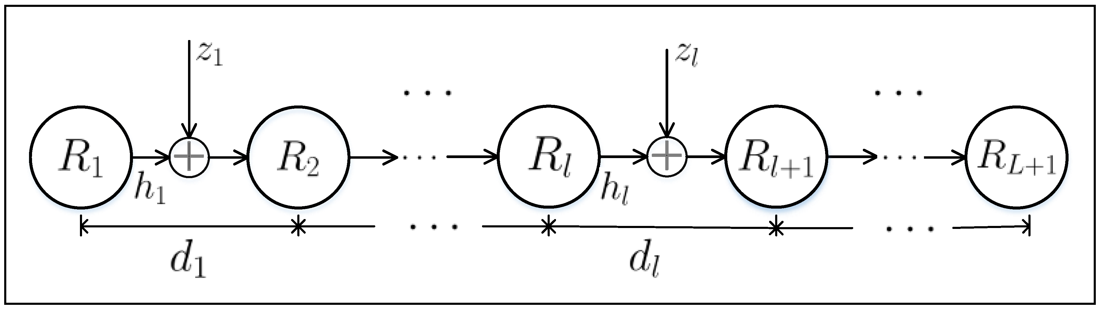
Figure 2.
Absolute values of AWGN samples with (top figure) and Middleton’s Class-A noise samples with , , (bottom figure).
Figure 2.
Absolute values of AWGN samples with (top figure) and Middleton’s Class-A noise samples with , , (bottom figure).

Figure 3.
Absolute values of Middleton’s Class-A noise samples with , , (top figure) and with , , (bottom figure).
Figure 3.
Absolute values of Middleton’s Class-A noise samples with , , (top figure) and with , , (bottom figure).

Figure 4.
End-to-end average BER of the L-hop relay network versus individual-hop average BER.
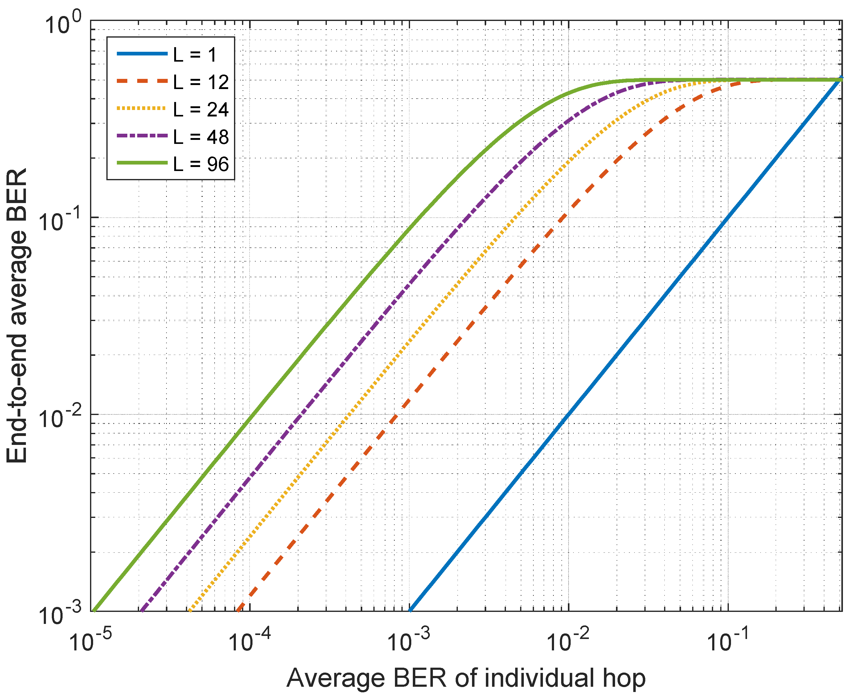
Figure 5.
End-to-end average BER vs. average SNR per link over Nakagami-m () channels with various noise conditions.
Figure 5.
End-to-end average BER vs. average SNR per link over Nakagami-m () channels with various noise conditions.

Figure 6.
End-to-end average BER v.s. average SNR per channel in the scenarios of Rayleigh fading () and no fading ().
Figure 6.
End-to-end average BER v.s. average SNR per channel in the scenarios of Rayleigh fading () and no fading ().
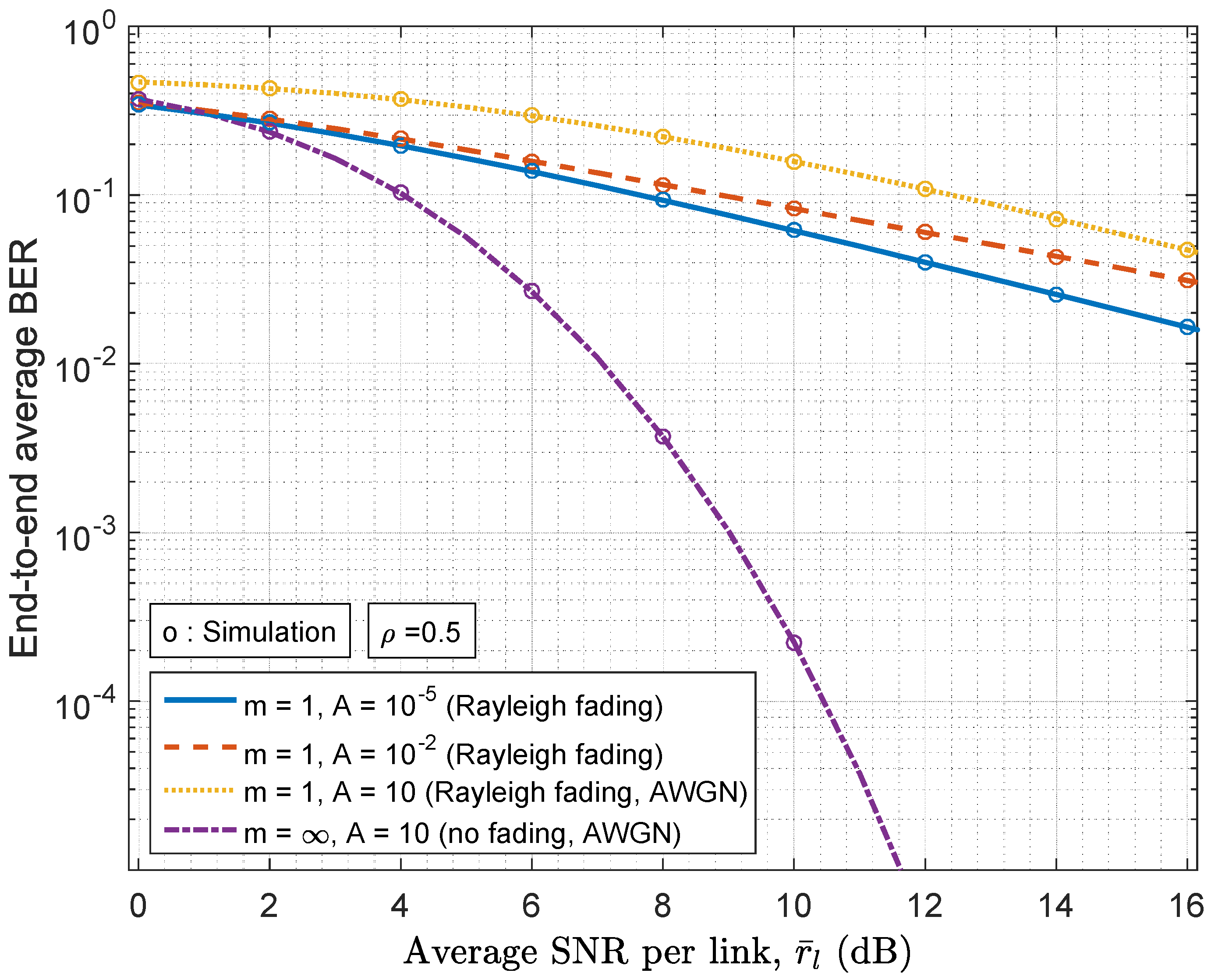
Figure 7.
End-to-end average BER vs. MCA impulsive index A for various values of and the Nakagami m parameter.
Figure 7.
End-to-end average BER vs. MCA impulsive index A for various values of and the Nakagami m parameter.

Figure 8.
End-to-end average BER vs. total transmission power for different values of MCA impulsive index A and path-loss exponent with (a) equal power allocation; (b) allocation scheme under (4).
Figure 8.
End-to-end average BER vs. total transmission power for different values of MCA impulsive index A and path-loss exponent with (a) equal power allocation; (b) allocation scheme under (4).
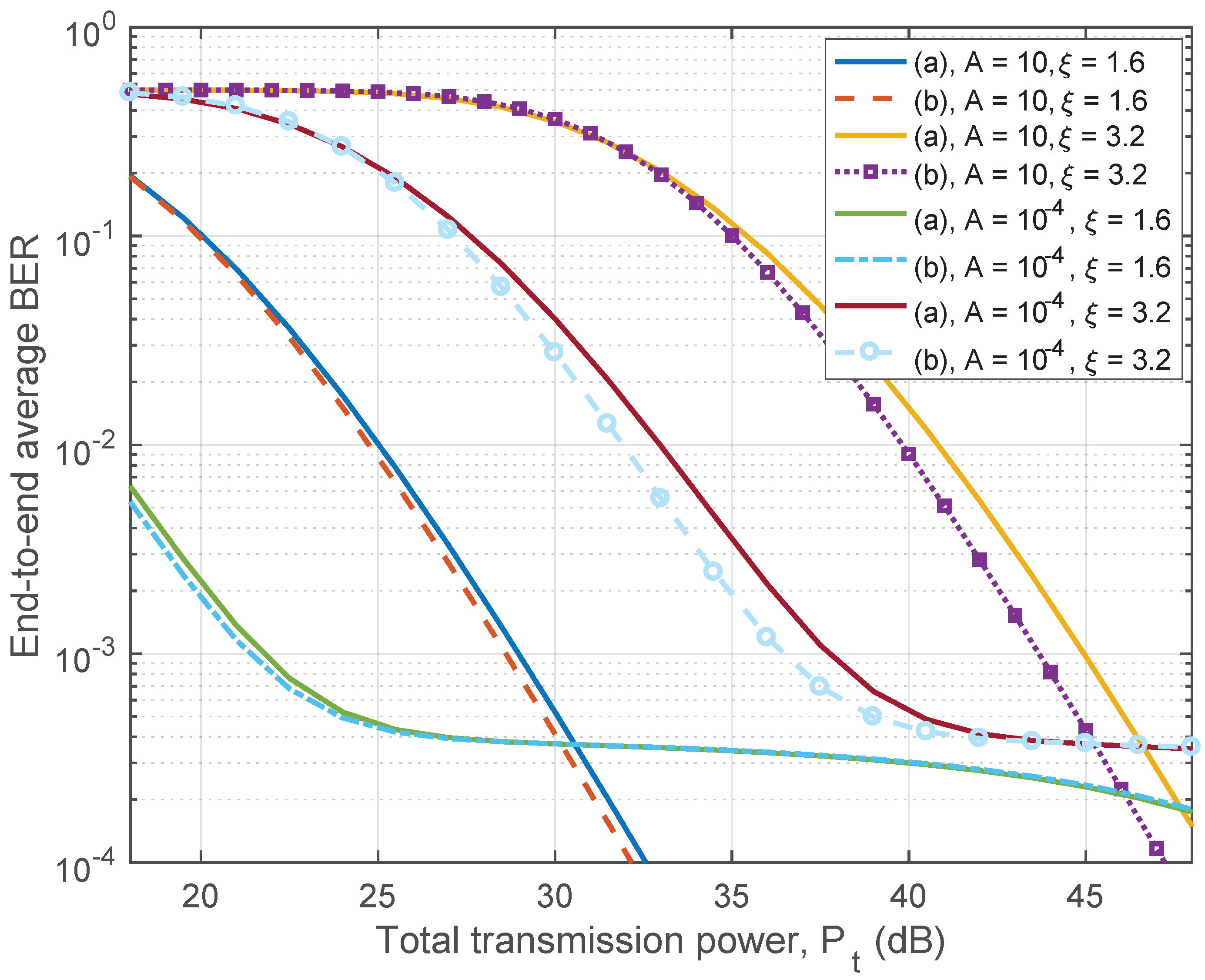
Figure 9.
The channel capacity of Nakagami-m channels () with relay hops.
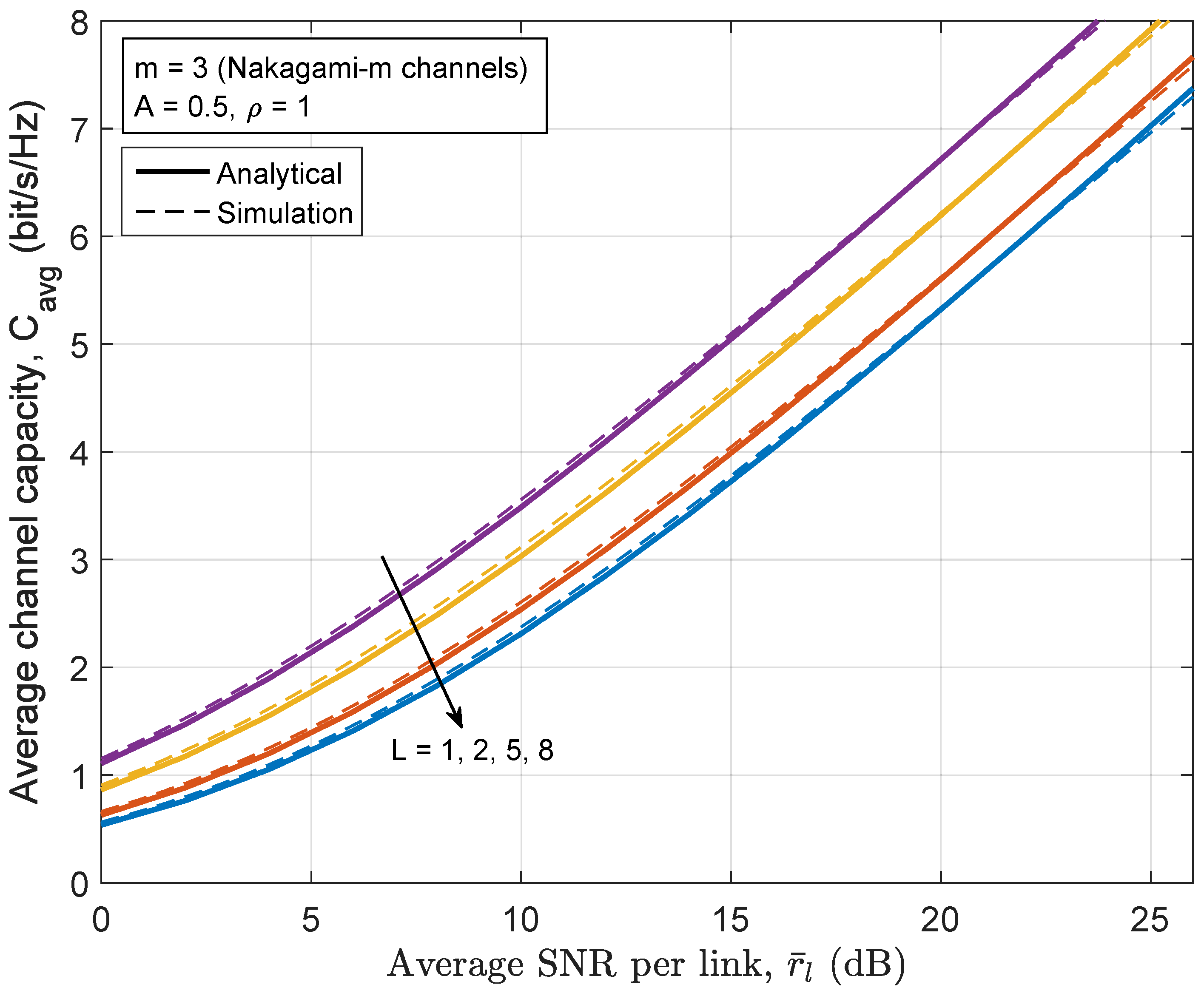
Figure 10.
The channel capacity of Rayleigh channels () and nearly AWGN () with relay hops.

Figure 11.
The PDF of channel capacity of Rayleigh channels () and Nakagami-m channels () with relay hops.
Figure 11.
The PDF of channel capacity of Rayleigh channels () and Nakagami-m channels () with relay hops.

Figure 12.
The variance of channel capacity for the relay fading channels with different values of m and L, .
Figure 12.
The variance of channel capacity for the relay fading channels with different values of m and L, .

© 2017 by the authors. Licensee MDPI, Basel, Switzerland. This article is an open access article distributed under the terms and conditions of the Creative Commons Attribution (CC BY) license (http://creativecommons.org/licenses/by/4.0/).
Share and Cite
MDPI and ACS Style
Ai, Y.; Cheffena, M. On Multi-Hop Decode-and-Forward Cooperative Relaying for Industrial Wireless Sensor Networks. Sensors 2017, 17, 695. https://doi.org/10.3390/s17040695
AMA Style
Ai Y, Cheffena M. On Multi-Hop Decode-and-Forward Cooperative Relaying for Industrial Wireless Sensor Networks. Sensors. 2017; 17(4):695. https://doi.org/10.3390/s17040695
Chicago/Turabian StyleAi, Yun, and Michael Cheffena. 2017. "On Multi-Hop Decode-and-Forward Cooperative Relaying for Industrial Wireless Sensor Networks" Sensors 17, no. 4: 695. https://doi.org/10.3390/s17040695
Note that from the first issue of 2016, this journal uses article numbers instead of page numbers. See further details here.