Article

Measuring Dynamic Signals with Direct Sensor-to-Microcontroller Interfaces Applied to a Magnetoresistive Sensor

1
Department of Computer and Electrical Engineering, Universidad Autónoma de Ciudad Juárez (UACJ), 32310 Ciudad Juárez, Mexico
2
e-CAT Research Group, Department of Electronic Engineering, Universitat Politècnica de Catalunya (UPC)—BarcelonaTech, C/Esteve Terradas 7, C4, 08860 Castelldefels, Spain
*
Author to whom correspondence should be addressed.
Sensors 2017, 17(5), 1150; https://doi.org/10.3390/s17051150
Submission received: 6 April 2017 / Revised: 9 May 2017 / Accepted: 15 May 2017 / Published: 18 May 2017
(This article belongs to the Special Issue Autonomous Sensors)

Abstract

:
This paper evaluates the performance of direct interface circuits (DIC), where the sensor is directly connected to a microcontroller, when a resistive sensor subjected to dynamic changes is measured. The theoretical analysis provides guidelines for the selection of the components taking into account both the desired resolution and the bandwidth of the input signal. Such an analysis reveals that there is a trade-off between the sampling frequency and the resolution of the measurement, and this depends on the selected value of the capacitor that forms the RC circuit together with the sensor resistance. This performance is then experimentally proved with a DIC measuring a magnetoresistive sensor exposed to a magnetic field of different frequencies, amplitudes, and waveforms. A sinusoidal magnetic field up to 1 kHz can be monitored with a resolution of eight bits and a sampling frequency of around 10 kSa/s. If a higher resolution is desired, the sampling frequency has to be lower, thus limiting the bandwidth of the dynamic signal under measurement. The DIC is also applied to measure an electrocardiogram-type signal and its QRS complex is well identified, which enables the estimation, for instance, of the heart rate.

1. Introduction

In the society of the 21st century, almost everything (e.g., home appliances, mobile phones, cars, buildings, and cities) is becoming “smart” thanks to the proliferation of information and communication technology and the deployment of technologies, such as wireless sensor networks and the Internet of things. To become smart, it is essential, in the first place, to monitor through sensors what is happening in and/or around the smart thing. The data collected is processed and then a smart decision is taken with the aim of improving the safety, efficiency, sustainability, mobility, etc. of the smart thing and, hence, the people’s quality of life.
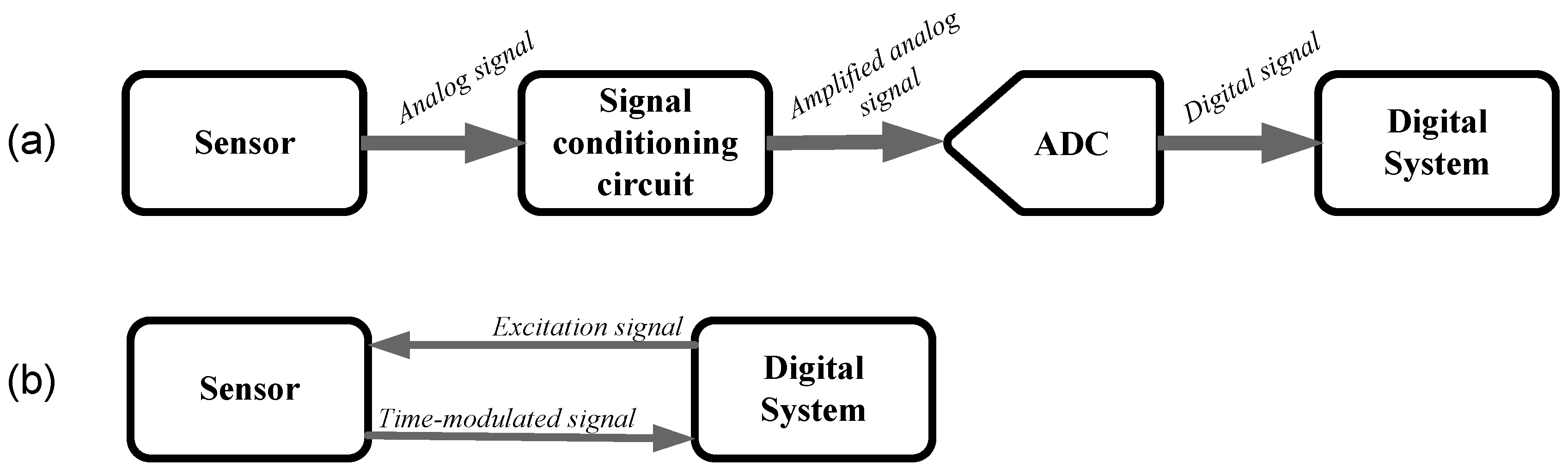
Sensors are electronic devices that provide an output signal in the electrical domain (e.g., resistance, capacitance, voltage, or current) with information about the measurand. However, such an electrical signal is generally of low amplitude and carries some noise and, therefore, an electronic interface is required between the sensor and the processing digital system so as to correctly extract the information of interest. A classical block diagram of an electronic sensor interface is shown in Figure 1a. The sensor output signal is first processed in the analog domain by a signal conditioning circuit that generally relies on operational amplifiers. The main functions of this block are level shifting and amplification so as to match the sensor output span to the input span of the ensuing analog-to-digital converter (ADC) and, hence, to make good use of the ADC dynamic range. Other common tasks of the signal conditioning circuit are: sensor output-to-voltage conversion, filtering, linearization, and/or demodulation. The resulting analog signal is then digitized via the ADC. Finally, a digital system acquires, stores, processes, controls, communicates (to other devices or systems) and/or displays the digital value with information about the measurand. Nowadays, the most popular digital systems are microcontrollers (μC) and field-programmable gate arrays (FPGA).
An alternative approach to reading some sensors (e.g., resistive [1,2,3,4], capacitive [5,6,7,8], inductive [9,10], and voltage-output [11,12] sensors) is shown in Figure 1b. This circuit topology is known as a direct interface circuit (DIC) since the sensor is directly connected to the digital system without using either the signal conditioning circuit or the ADC, thus resulting in a direct sensor-to-μC [13] or to-FPGA interface circuit [14,15]. In this topology, the digital system excites the sensor to obtain a time-modulated signal that is directly measured in the digital domain through a digital timer embedded into the digital system. In comparison with the sensor electronic interface shown in Figure 1a, a DIC is simpler and needs fewer components. Actually, it can be implemented with a common general-purpose 8-bit μC which is a low-cost (say, $1) and low-power (say, about 1 mA in active mode and less than 1 μA in power-down mode [16]) device. Modern μCs may also incorporate into the same chip an ADC that facilitates the design of the topology shown in Figure 1a, but an ADC demands more power than a digital timer. Therefore, a DIC based on a time-to-digital conversion [17,18] offers advantages in terms of cost, physical space, and power consumption, which is of major interest, for example, in autonomous sensors powered by either batteries or energy harvesters. Furthermore, the performance of such circuits, in terms of accuracy and resolution, is quite remarkable taking into account their simplicity, for instance: a non-linearity error of 0.01% full-scale span (FSS) and a resolution of 13 bits when measuring resistive sensors in the kilo-Ohm range [1], and 0.1% FSS and nine bits when measuring capacitive sensors in the picofarad range [5].
Although the performance and feasibility of DICs have been extensively analyzed and proved in the literature, these have been evaluated and then applied to measure static or quasi-static signals, i.e., slowly-varying magnitudes, such as temperature [1], relative humidity [5], or respiratory rate [19]. The analysis of the limitations and trade-offs of DICs when measuring sensors subjected to dynamic changes (e.g., vibrations, pulse rate, or alternating magnetic fields) have not been assessed so far. It has been widely thought that DICs were not able to measure such dynamic signals since they rely on measuring the charging or discharging time of an RC circuit, which can be quite long (say, units or tens of millisecond) if a high or medium resolution is required. This paper goes beyond these approaches and explores the feasibility of DICs to measure a resistive sensor with dynamic changes of resistance.
The paper is organized as follows. Section 2 qualitatively describes the operating principle of the DIC when measuring a resistive sensor. Section 3 theoretically analyzes the limitations and trade-offs of DICs in dynamic measurements. Section 4 describes the setup and the measurement method. Section 5 shows the experimental results and discusses them. Finally, Section 6 draws the main conclusions.

2. Operating Principle

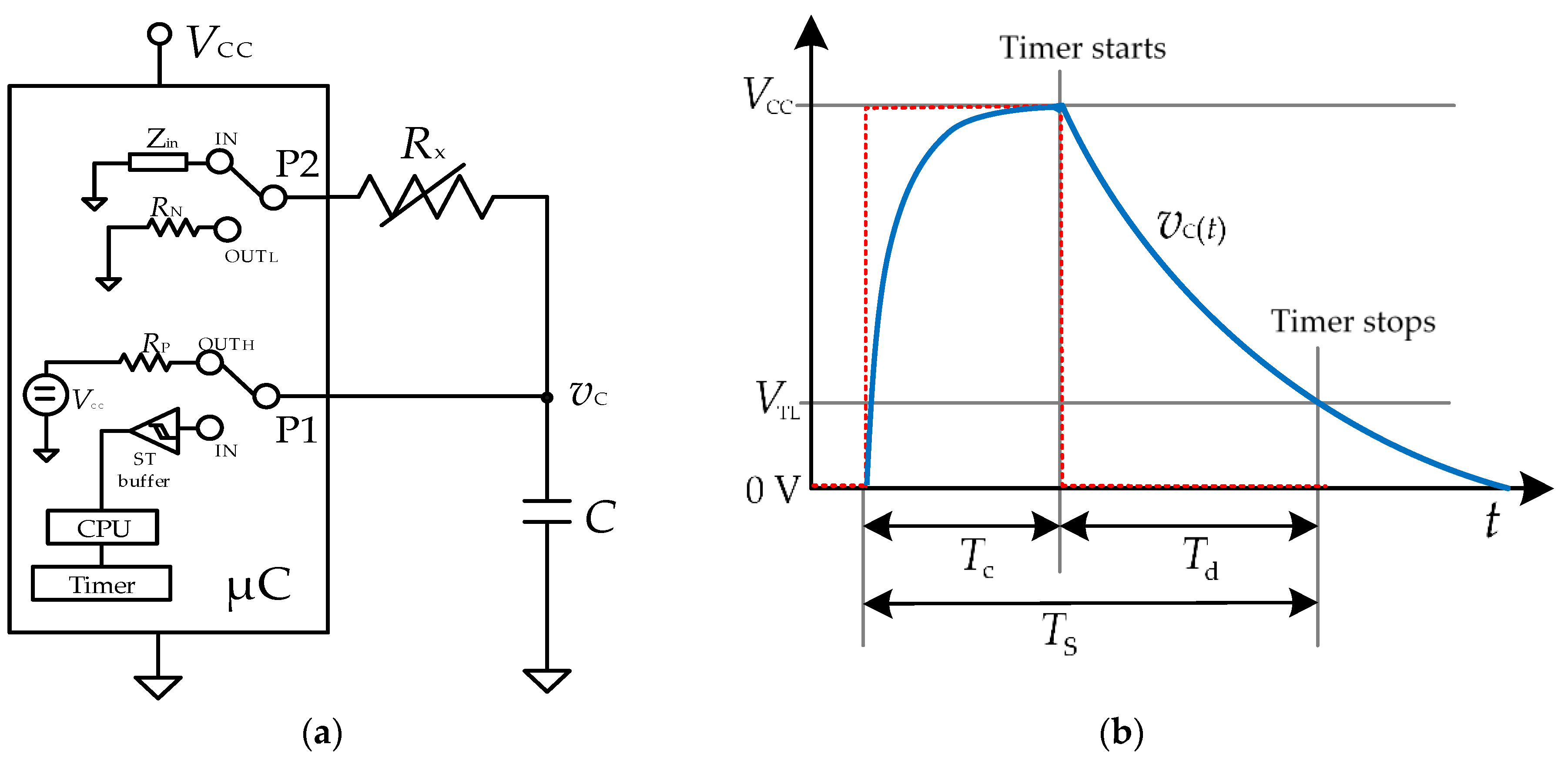
The basic topology of a μC-based DIC for the measurement of a resistive sensor (Rx) is shown in Figure 2a [13], where C is a capacitor to build an RC circuit, P1 and P2 are two input/output digital ports, and VCC is the supply voltage of the μC. The DIC estimates the value of Rx by measuring, through an embedded digital timer, the time interval needed to discharge C through Rx from VCC to a certain threshold voltage. In order to reduce the uncertainty of the time-interval measurement, it is advisable to employ a port P1 associated to a capture module (or an external interrupt) having a Schmitt trigger (ST) buffer with a low (VTL) and a high threshold voltage (VTH). The measurement of the discharging time of the RC circuit to extract the value of Rx is preferable than that of the charging time since the former uses VTL as a threshold voltage, which is less noisy than VTH [13].
The algorithm carried out by the µC to obtain a digital value proportional to Rx involves two operating stages: (a) charging, and (b) discharging and time measurement, as shown in Figure 2b. In the first stage, P1 is set as an output providing a digital “1”, while P2 is set as an input offering high impedance (HZ). Consequently, P1 generates a step pulse from 0 to VCC (i.e., from “0” to “1” in the digital domain) and, therefore, C is charged towards VCC through RP with a time constant τc = RPC, where RP represents the equivalent internal resistance of P1; RP is about tens of ohms [1], which is small enough to have a fast charge. This charging stage must last at least 5τc so as to ensure that the voltage across C (vc(t) in Figure 2b) has reached VCC. In the second stage, P2 is set as an output providing a digital “0”, while P1 is set in HZ waiting for the threshold-voltage crossing. In such conditions, C is discharged towards ground through Rx + RN with a time constant τd = (Rx + RN) C, where RN represents the equivalent internal resistance of P2. In the meantime, the embedded timer measures the time interval required to do so. When vc(t) reaches VTL, the ST buffer is triggered and the timer stops. The charging and discharging times are, respectively, equal to:
T c = 5 R P C
T d = ln ( V CC V TL ) ( R x + R N ) C
From Equation (1b), if C, VCC, VTL, and RN are assumed constant, then Td is proportional to Rx. The effects of the tolerance and low-frequency variability of these parameters can be compensated by adding reference components in the DIC and then applying auto-calibration techniques, as explained elsewhere [1,13]. In summary, the DIC first performs a resistance-to-time conversion and, then, a time-to-digital conversion, thus resulting in a digital number proportional to Td and, hence, to Rx.

3. Analysis of the Dynamic Performance

Let us assume that the sensor resistance is subjected to sinusoidal changes, as shown in Figure 3, and so it can be expressed as:
R x ( t ) = R x , 0 + Δ R x 2 sin 2 π f t
where Rx,0 is the nominal resistance at a reference value of the measurand, ΔRx is the peak-to-peak change of resistance (which is considered to be much smaller than Rx,0, say less than ±10%), and f is the frequency of the sinusoidal change.

3.1. Sampling Frequency

The DIC shown in Figure 2a takes a sample of Rx every Ts, as represented in Figure 3. This sampling period can be calculated as Tc + Td and, consequently, the sampling frequency is:
f s = 1 T s = 1 C [ 5 R P + ln ( V CC V TL ) ( R x , 0 + R N ) ]
Again, it is assumed that ΔRx << Rx,0 and, hence, fs can be considered almost independent of the measurand. If fs is high enough, which involves a low value of C, then the samples taken of Rx will enable the reconstruction of the dynamic signal affecting the sensor. Of course, the Nyquist criterion, which states that the signal must be sampled at least at twice the value of f, has to be satisfied. For a given application requiring a minimum value of fs, the maximum value of C can be calculated, from Equation (3), as:
C 1 f s [ 5 R P   +   ln ( V CC V TL ) ( R x , 0 + R N ) ]
which decreases with increasing fs.

3.2. Frequency Response

The RC circuit in Figure 2a behaves as a passive integrating circuit, so that the dynamic changes of resistance are expected to be filtered. As a consequence of the integration process during the discharging time, we propose to define a “filtered” value of Rx that can be expressed as:
R x , f = 1 T d t 0 t 0 + T d R x ( t ) d t
where t0 is the instant at which the discharging stage starts. Inserting Equation (2) into Equation (5) yields:
R x , f = R x , 0 + Δ R x 2 sin π f T d π f T d sin [ 2 π f t 0 + π f T d ] Term 1
Each measurement of the discharging time involves a different value of t0 and, hence, Term1 in Equation (6) can have any value between −1 and 1. Therefore, Rx,f in Equation (6) undergoes a resistance change whose amplitude can be normalized as follows:
Δ R x , f Δ R x = | sin π f T d | π f T d
According to Equation (7), the measurement is subjected to a sinc-based low-pass filter (LPF) response, which involves zeros at specific values of frequency. This is similar to the performance obtained in integrating ADCs when rejecting interference superimposed on the input signal to be digitized [20], or in quasi-digital sensors when rejecting interference superimposed on the supply voltage [21,22]. Assuming common values of Rx, RN, and RP, we have Td >> Tc, and then TsTd and, consequently, Equation (7) can be rewritten as:
Δ R x , f Δ R x | sin π f / f s | π f / f s
which is represented in Figure 4 showing a maximum attenuation when f is a multiple of fs. The principal lobe of the response shown in Figure 4 determines the bandwidth of the DIC. At the Nyquist frequency (i.e., f = 0.5fs), the attenuation factor is 3.9 dB. If fs = 10f, which will be under test in Section 5, then the attenuation factor is 0.1 dB.

3.3. Resolution

A DIC for a resistive sensor with n bits is expected to provide a resolution in ohms equal to:
Δ r = Δ R x , max 2 n
where ΔRx,max is the maximum value of ΔRx for a given application. On the other hand, the digital timer that measures the discharging time has a timing resolution equal to the period (T0) of its reference oscillator; this is assuming that the uncertainty in the timing process is mainly due to quantization effects, which is valid if the value of C is not very high (say, smaller than 1 μF) [23]. Accordingly, the change in the discharging time caused by Δr must be at least longer than T0. Consequently, from Equations (1b) and (9), we can find the minimum value of C to achieve n bits:
C     T 0 2 n ln ( V CC V TL ) Δ R x , max
which increases with increasing n.

3.4. Trade-Offs

According to the previous subsections, there is a trade-off between the sampling frequency and the resolution of the measurement. The higher the value of fs, which involves a low value of C, the lower the resolution. On the contrary, the higher the resolution, which implicates a high value of C, the lower the value of fs. For instance, Table 1 shows the effects of different values of C on both the sampling frequency and the resolution, considering Rx,0 = 743 Ω, ΔRx,max = 120 Ω (i.e., ±8%), VCC = 5.20 V, VTL = 1.76 V, RP = 24 Ω, RN = 28 Ω, and T0 = 62.5 ns, which are the experimental values employed later in Section 4 and Section 5. For a given application requiring n bits of resolution and a sampling frequency of fs, the value of C should be, combining Equations (4) and (10), within the following range:
T 0 2 n ln ( V CC V TL ) Δ R x , max C 1 f s [ 5 R P + ln ( V CC V TL ) ( R x , 0 + R N ) ]
On the other hand, we also have the attenuation factor affecting the dynamic change of resistance that depends on the ratio f/fs. As C decreases, so does the ratio f/fs and, hence, the attenuation factor caused by the inherent LPF shown in Figure 4. Therefore, from the range of potential values of C resulting from Equation (11), it is advisable to select the smallest one so as to minimize such attenuation.
Another trade-off is present with regard to the effects of T0 on the performance of the DIC. The lower the value of T0, the lower the minimum value of C to achieve n bits and, hence, the higher the maximum sampling frequency. This also has benefits in terms of cost since low-value capacitors are generally less expensive. However, a low value of T0 requires a high-frequency reference oscillator, which involves a higher power consumption and can generate more trigger noise, affecting the threshold-voltage crossing.

4. Materials and Method

The DIC shown in Figure 2a has been implemented using a commercial 8-bit μC (ATmega328, Atmel, San Jose, CA, USA) running at 16 MHz and powered at +5 V. This supply voltage was provided by an independent voltage regulator (LM2940) to reduce the power supply noise/interference that may generate trigger noise affecting the discharging-time measurement [1]. The tasks of P1 and P2 in Figure 2a were carried out by PD2 and PB3, respectively. An embedded 16-bit digital timer was employed to measure the discharging time with T0 = 62.5 ns. The central processing unit (CPU) of the μC was placed in sleep mode (but the timer and the interrupt system kept working) during the discharging-time measurement to decrease the internal trigger noise generated by the CPU itself. The μC was programmed to acquire and save (in RAM) 250 samples of Td corresponding to 250 samples of Rx. These samples were then sent via USB to a personal computer controlled by a LabVIEW program. The values of Td were then converted into Rx through Equation (1b), and assuming the values of VCC, VTL, RP, and RN as indicated before in
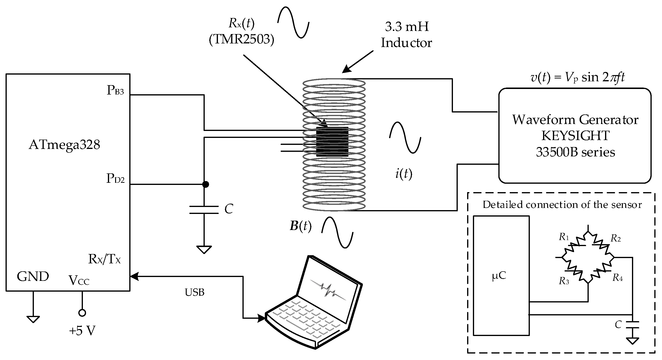
 Section 3.4
The sensor under test was a magnetoresistive sensor (TMR2503, MDT, Jiangsu, China) exposed to an alternating magnetic field, B(t), that was generated by an inductor of 3.3 mH excited by a waveform generator (33500B, Keysight Technologies, Santa Rosa, CA, USA), as shown in Figure 5. The sensor was placed near the inductor with its surface perpendicular to the generated magnetic field. The TMR2503 has four magnetoresistances connected in a Wheatstone bridge topology, but only a single equivalent resistance of the sensor was measured. To be precise, the equivalent resistance was one of the magnetoresistances (R4) in parallel with the series combination of the other three (R1, R2, and R3), as shown in Figure 5 in the dashed-line box. This equivalent resistance can be considered proportional to the magnetic field if the relative variation of resistance is much smaller than one [3].
Two preliminary tests on the TMR2503 were initially conducted. The first test was intended to obtain the transfer curve (i.e., Rx versus B) of the sensor. To do so, the inductor was excited by a DC voltage source (2230G-30-1, Keithley Instruments, Cleveland, OH, USA) to generate a DC magnetic field that was measured by a magnetometer (Mag-01H, Bartington Instruments, Witney, UK), and the sensor equivalent resistance was measured by a digital multimeter (2110, Keithley Instruments, Cleveland, OH, USA). The second test was intended to monitor the sensor output signal through a classical read-out circuit when a sinusoidal magnetic field of 1 kHz was applied. In such a case, the sensor was supplied at 5 V and its differential output voltage was amplified by an instrumentation amplifier (AD620, Analog Devices, Norwood, MA, USA) with a gain of 100. The output signal of the amplifier was acquired by a digital oscilloscope (DSOX2014A, Keysight Technologies, Santa Rosa, CA, USA).
The dynamic performance of the DIC was then tested using the measurement set-up shown in Figure 5, which enables to change the frequency, amplitude, and waveform of B(t) and that of Rx(t). Three different experiments were carried out:
(a)
Experiment A, which was intended to observe the effects of frequency. The frequency of B(t) was varied from 10 Hz to the Nyquist frequency, the amplitude was the maximum (corresponding to a peak-to-peak amplitude of 20 V from the generator), and the waveform was sinusoidal. Three different values of C were tested: 100 nF, 330 nF, and 680 nF.
(b)
Experiment B, which was intended to observe the effects of amplitude. The frequency of B(
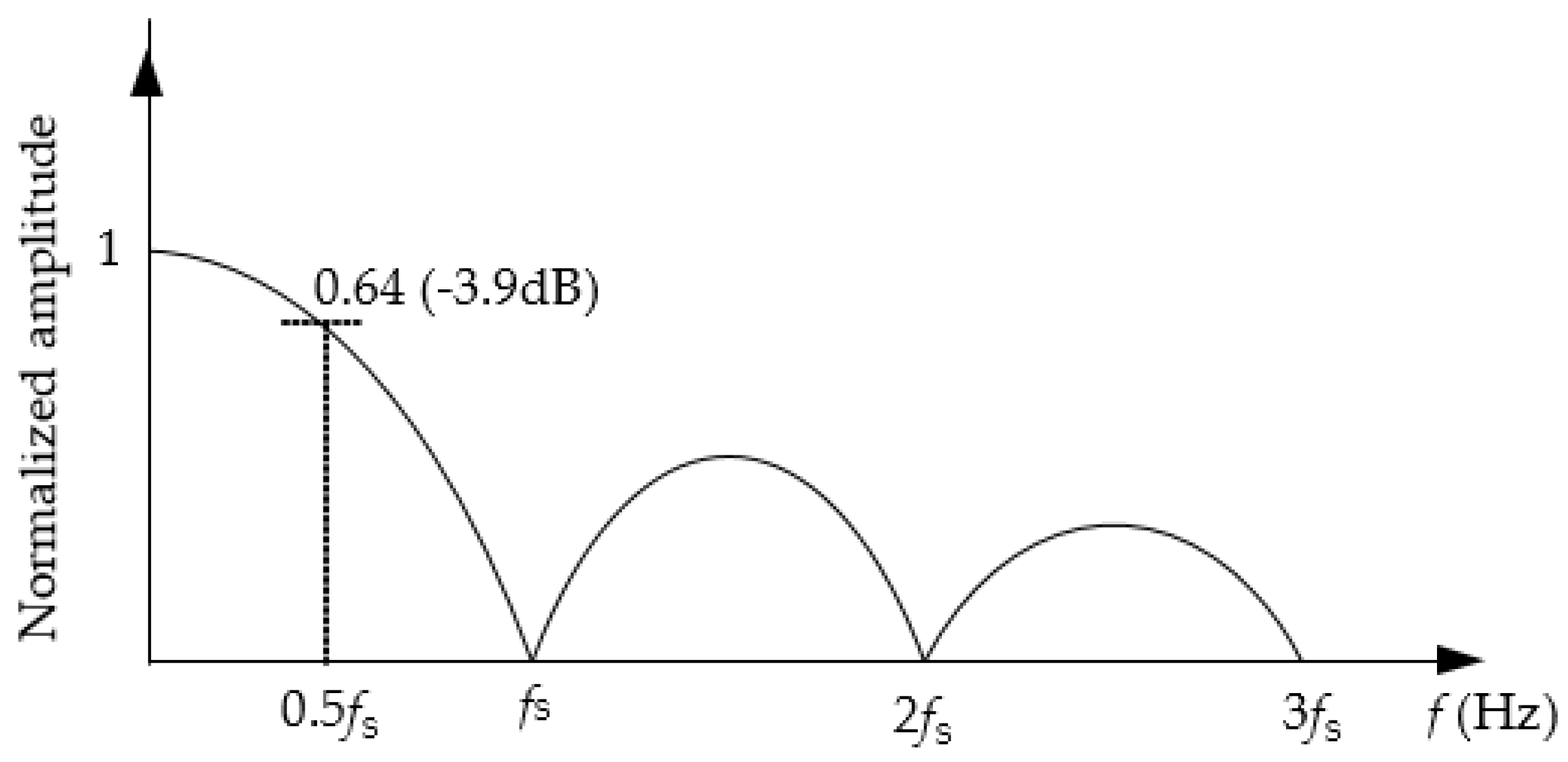
t) was constant, the amplitude had three different levels (corresponding to a peak-to-peak amplitude of 5, 10, and 20 V from the generator), and the waveform was sinusoidal. A frequency of 1 kHz and a capacitor of 100 nF were selected. As shown later after presenting the results of Experiment A, this is the highest frequency that can be tested without the effects of the inherent LPF; note, from Table 1, that fs ≈ 10f when C = 100 nF and, hence, the attenuation factor is 0.1 dB. A higher frequency value could be tested using a smaller value of C, but then the resolution would be smaller than eight bits, which is usually considered as the minimum value in electronic instrumentation.
(c)
Experiment C, which was intended to observe the effects of the waveform. The inductor was excited with a narrowband signal with different amplitudes and frequency components. To be precise, the excitation signal emulated an electrocardiogram (ECG) signal with a fundamental frequency of 1.5 Hz that corresponds to a heart rate of 90 beats per minute. ECG monitoring requires a read-out circuit whose bandwidth should be no less than 40 Hz [24]. In order to have such a bandwidth and also optimize the performance of the DIC in terms of resolution, a capacitor of 4.7 μF was selected. This capacitor provides, from Equation (3), a sampling frequency of around 200 Sa/s and, from Equation (8), a 3-dB cut-off frequency of 90 Hz. The ECG signal applied to the inductor was also monitored by the digital oscilloscope.

5. Experimental Results and Discussion

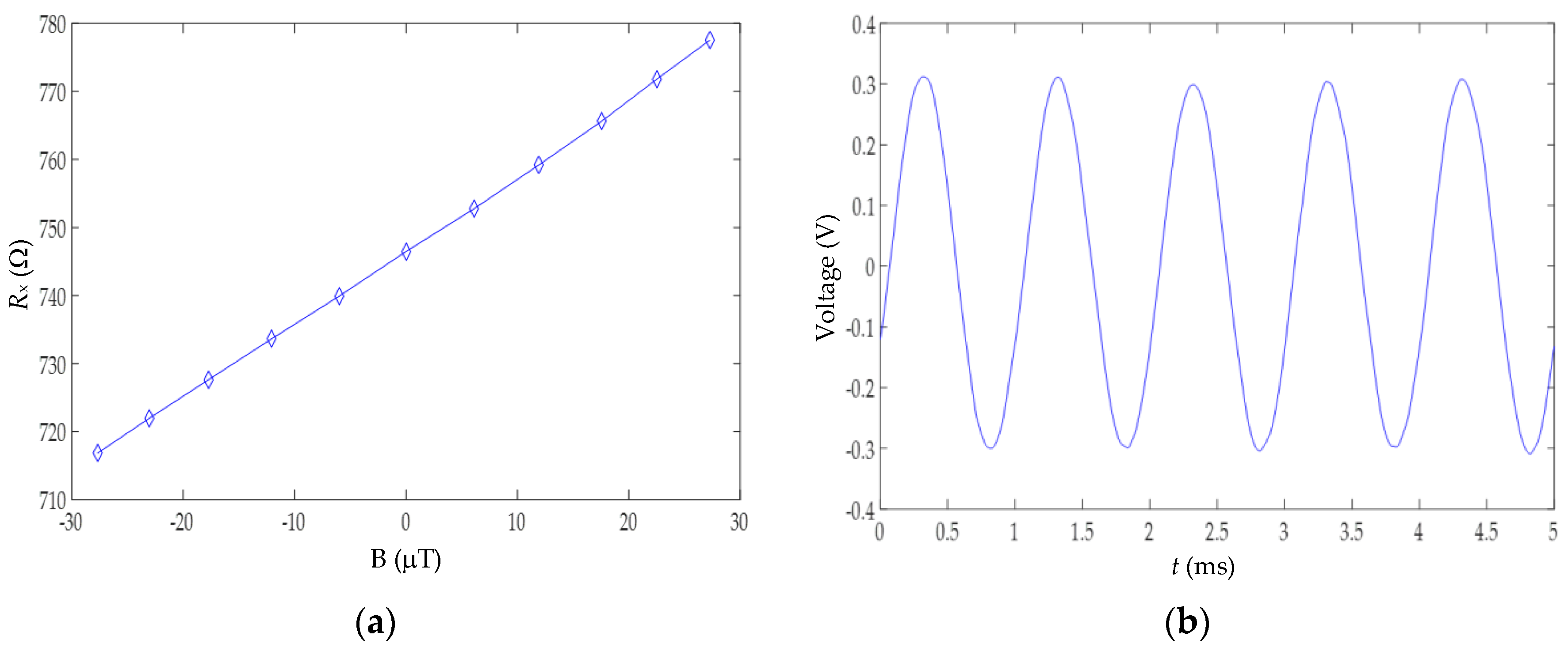
Figure 6 shows the results obtained in the preliminary tests of the magnetoresistive sensor. On the one hand, Figure 6a shows the transfer curve of the sensor for a DC magnetic field ranging from −30 μT to +30 μT. According to these experimental results, we can confirm that the sensor equivalent resistance linearly changes with the magnetic field applied. On the other hand, Figure 6b shows the output signal in the time domain when the sensor (subjected to a sinusoidal magnetic field of 1 kHz) was measured by a classical read-out circuit. The resulting signal was also sinusoidal with the same frequency as that of the magnetic field applied, as expected, and without experiencing any kind of saturation problems.
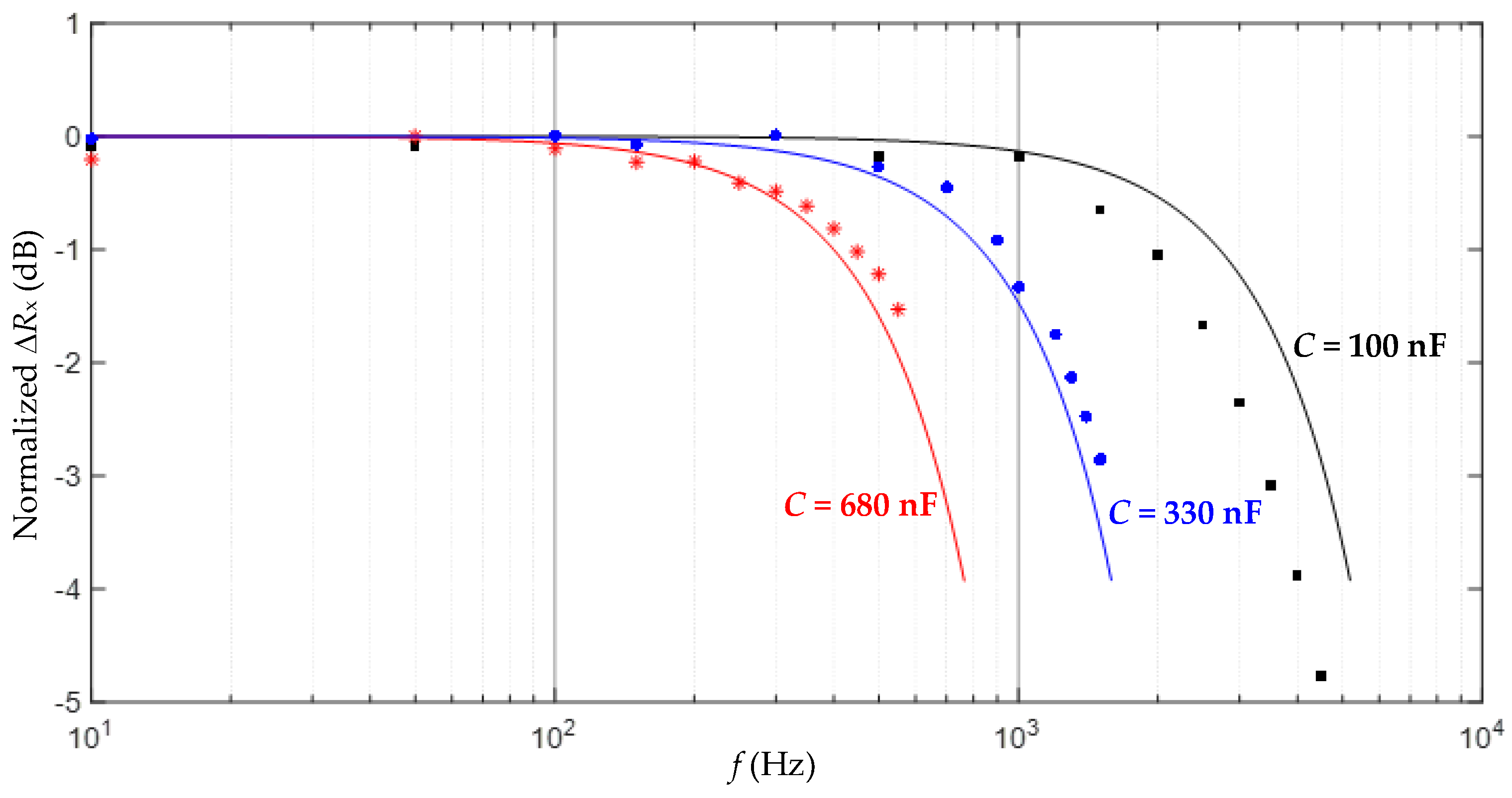
The results obtained in the experiment A are represented in Figure 7, where the y-axis shows the value of ΔRx normalized to that obtained at 10 Hz and expressed in dB. The results in Figure 7 show that the measurement suffers from a LPF behavior that limits the bandwidth of the dynamic signal to be sensed, as suggested before in Section 3.2. The theoretical frequency response predicted by Equation (8) is also represented (as a solid line) in Figure 7, which shows good agreement with the experimental data. As C increased, both fs and the bandwidth decreased, as predicted before by Equation (3) and Figure 4, respectively. According to Figure 7, if the DIC has to measure, for instance, resistance variations at 1 kHz, it is advisable to employ a capacitor of 100 nF, which limits the resolution to around eight bits. Resistance variations at frequencies higher than 1 kHz would require a lower value of C in order to avoid the effects of the inherent LFP, but then the resolution would be lower than eight bits.
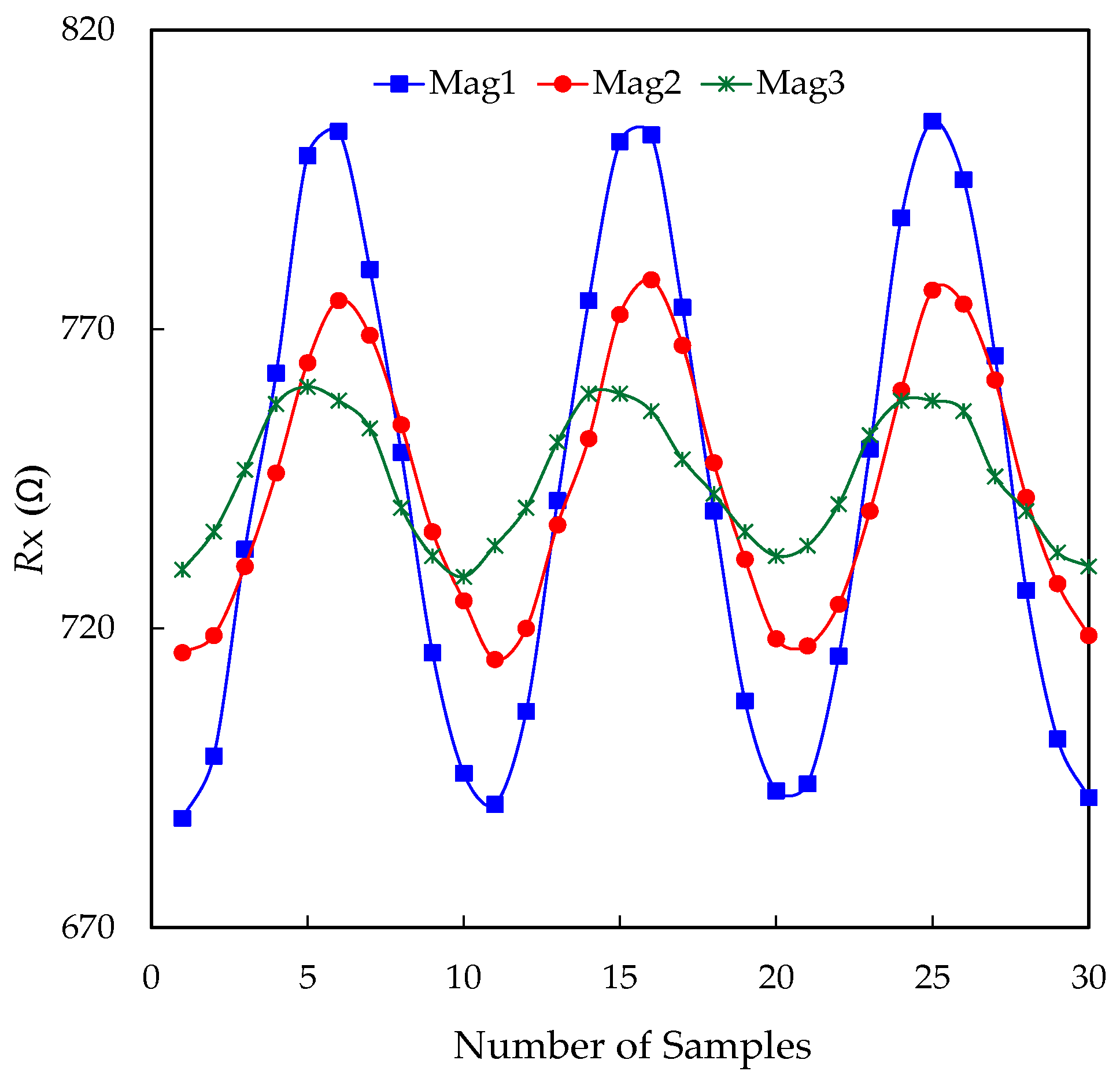
Figure 8 shows the results achieved in the experiment B. First of all, the frequency of 1 kHz under test was located in the pass band of the LPF, as shown in Figure 7 for C = 100 nF. Second of all, the experimental value of fs was 10.2 kSa/s, which was high enough to measure a signal of 1 kHz; in other words: around 10 samples per period were taken. The three levels of the magnetic field applied to the sensor (represented in Figure 8 as “Mag1”, “Mag2”, and “Mag3”, being Mag1 > Mag2 > Mag3) caused a ΔRx of 120 Ω, 66 Ω, and 36 Ω, respectively. If Mag1 is assumed to be the maximum magnetic field under measurement, then Δr = 577 mΩ, as reported before in Table 1, which generates quantization effects that are more evident when measuring low-amplitude signals. This is shown, for instance, in Figure 8 for the Mag3 case, where two consecutive samples taken close to the maximum of the sinusoidal signal have the same measurement result; in other words: the DIC was not able to detect the resistance change between these two samples. For this reason, the “sinusoidal” signal reconstructed from the samples was more distorted for Mag3 than for Mag1.
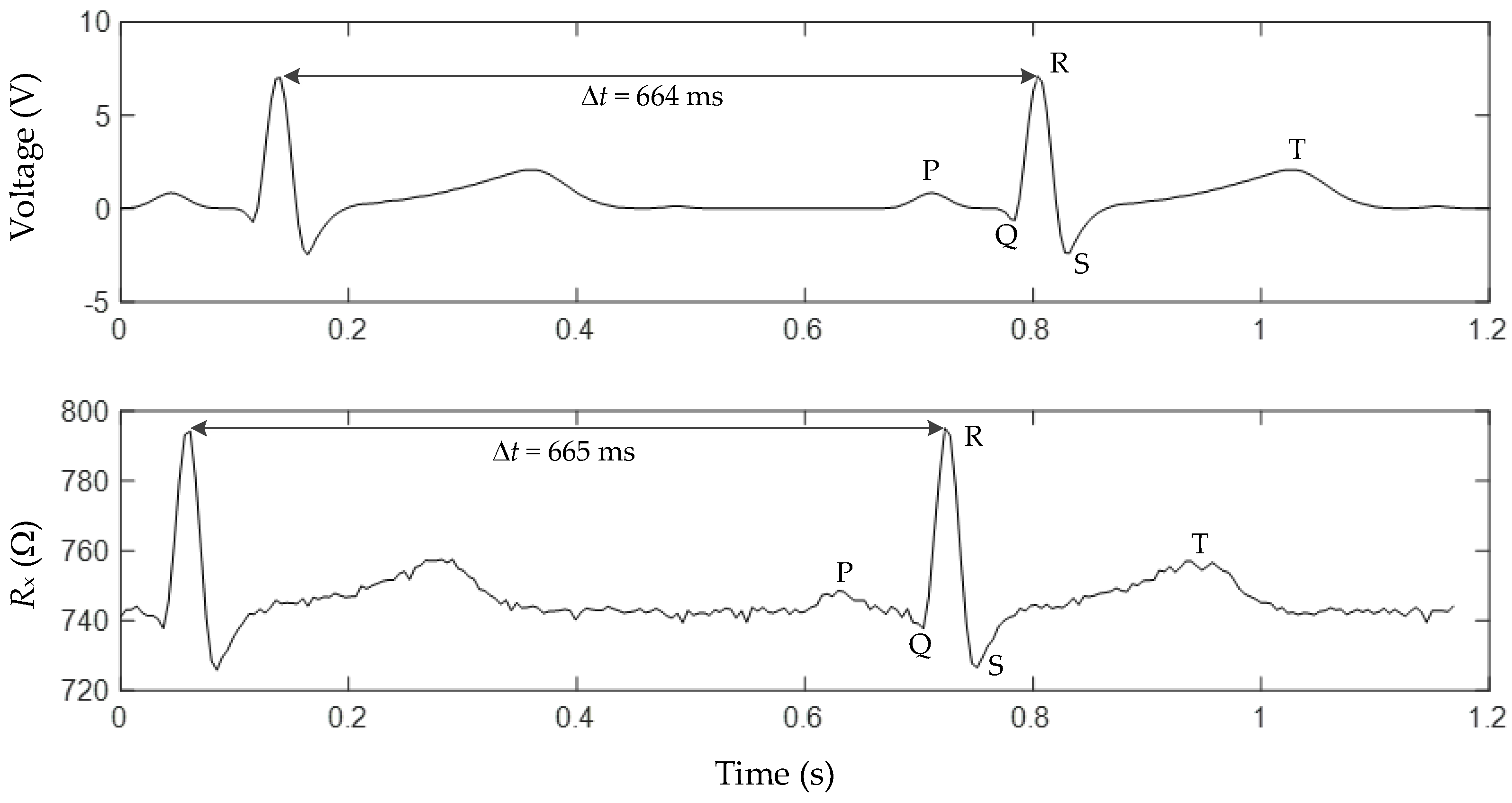
The results from the experiment C are shown in Figure 9. The ECG signal was acquired by the oscilloscope operating at 250 Sa/s (upper trace in Figure 9) and by the DIC at 200 Sa/s (bottom trace in Figure 9). The signal reconstructed from the samples acquired by the DIC was very similar to the original one monitored by the oscilloscope. For the highest amplitudes (QRS complex of the ECG [25]), the shape of the reconstructed wave was well preserved and, hence, it was possible to estimate the fundamental frequency (i.e., 1.5 Hz) of this periodic signal. However, for low amplitudes (e.g., T and P wave of the ECG), the reconstruction of the signal was slightly distorted, as also observed before in Figure 8 for the Mag3 case. The results in Figure 9 demonstrate that a DIC can not only measure dynamic signals with a sinusoidal behavior, but also more complex signals with a limited bandwidth.

6. Conclusions

This work has gone a step further in the field of DICs based on a RC circuit by applying them to measure a resistive sensor subjected to dynamic changes. The limitations and trade-offs have been identified and theoretically analyzed. It is remarkable the fact that the RC circuit not only generates a discharging time with information about the sensor resistance, but it also causes a sinc-based LPF behavior that limits the bandwidth. It has been shown that there is a trade-off between the sampling frequency and the resolution of the measurement, and this depends on the selected value of the capacitor of the RC circuit. Experimental tests have been carried out through a commercial microcontroller measuring a magnetoresistive sensor exposed to a magnetic field of different frequencies, amplitudes, and waveforms. According to these experimental results, sinusoidal variations of resistance with a frequency up to 1 kHz can be acquired with a resolution of eight bits. The capability of the DIC to monitor signals with a more complex waveform, such as an ECG signal, has also been demonstrated. The QRS complex of this ECG signal has been well identified and, therefore, the heart rate could be easily estimated.

Acknowledgments

Ernesto Sifuentes, Rafael González-Landaeta, and Juan Cota-Ruiz have been funded by PRODEP and UACJ, Mexico. The work of Ferran Reverter was supported by the Spanish Ministry of Economy and Competitiveness and the European Regional Development Fund under project TEC2016-76991-P.

Author Contributions

Ernesto Sifuentes and Rafael Gonzalez-Landaeta proposed the main idea, wrote the first version of the manuscript and, together with Juan Cota-Ruiz, built the measurement setup, performed the experiments, and analyzed the data. Ferran Reverter developed the theoretical models, interpreted the results, and revised the writing of the manuscript. All of the authors approved the final version of the manuscript.

Conflicts of Interest

The authors declare no conflict of interest.

References

  1. Reverter, F.; Jordana, J.; Gasulla, M.; Pallàs-Areny, R. Accuracy and resolution of direct resistive sensor-to-microcontroller interfaces. Sens. Actuators A Phys. 2005, 121, 78–87. [Google Scholar] [CrossRef]
  2. Reverter, F.; Casas, O. Interfacing differential resistive sensors to microcontrollers: A direct approach. IEEE Trans. Instrum. Meas. 2009, 58, 3405–3410. [Google Scholar] [CrossRef]
  3. Sifuentes, E.; Casas, O.; Reverter, F.; Pallas-Areny, R. Direct interface circuit to linearise resistive sensor bridges. Sens. Actuators A Phys. 2008, 147, 210–215. [Google Scholar] [CrossRef]
  4. Ponnalagu, R.N.; George, B.; Kumar, V.J. A microcontroller sensor interface suitable for resistive sensors with large lead resistance. In Proceedings of the 8th International Conference Sensing Technology, Liverpool, UK, 2–4 September 2014; pp. 327–331. [Google Scholar]
  5. Reverter, F.; Casas, O. Direct interface circuit for capacitive humidity sensors. Sens. Actuators A Phys. 2008, 143, 315–322. [Google Scholar] [CrossRef]
  6. Reverter, F.; Casas, O. Interfacing differential capacitive sensors to microcontrollers: A direct approach. IEEE Trans. Instrum. Meas. 2010, 59, 2763–2769. [Google Scholar] [CrossRef]
  7. Pelegrí-Sebastiá, J.; García-Breijo, E.; Ibáñez, J.; Sogorb, T.; Laguarda-Miro, N.; Garrigues, J. Low-cost capacitive humidity sensor for application within flexible RFID labels based on microcontroller systems. IEEE Trans. Instrum. Meas. 2012, 61, 545–553. [Google Scholar] [CrossRef]
  8. Chetpattananondh, K.; Tapoanoi, T.; Phukpattaranont, P.; Jindapetch, N. A self-calibration water level measurement using an interdigital capacitive sensor. Sens. Actuators A Phys. 2014, 209, 175–182. [Google Scholar] [CrossRef]
  9. Kokolanski, Z.; Jordana, J.; Gasulla, M.; Dimcev, V.; Reverter, F. Direct inductive sensor-to-microcontroller interface circuit. Sens. Actuators A Phys. 2015, 224, 185–191. [Google Scholar] [CrossRef]
  10. Ramadoss, N.; George, B. A simple microcontroller based digitizer for differential inductive sensors. In Proceedings of the IEEE International Instrumentation Measurement Technology Conference, Pisa, Italy, 11–14 May 2015. [Google Scholar]
  11. Bengtsson, L. Direct analog-to-microcontroller interfacing. Sens. Actuators A Phys. 2012, 179, 105–113. [Google Scholar] [CrossRef]
  12. Dutta, L.; Hazarika, A.; Bhuyan, M. Microcontroller based e-nose for gas classification without using ADC. Sens. Transducers 2016, 202, 38–45. [Google Scholar]
  13. Reverter, F. The art of directly interfacing sensors to microcontrollers. J. Low Power Electron. Appl. 2012, 2, 265–281. [Google Scholar] [CrossRef]
  14. Oballe-Peinado, O.; Vidal-Verdú, F.; Sánchez-Durán, J.A.; Castellanos-Ramos, J.; Hidalgo-López, J.A. Accuracy and resolution analysis of a direct resistive sensor array to FPGA interface. Sensors 2016, 16, 181. [Google Scholar] [CrossRef] [PubMed]
  15. Oballe-Peinado, O.; Vidal-Verdú, F.; Sánchez-Durán, J.A.; Castellanos-Ramos, J.; Hidalgo-López, J.A. Smart capture modules for direct sensor-to-FPGA interfaces. Sensors 2015, 15, 31762–31780. [Google Scholar] [CrossRef] [PubMed]
  16. Reverter, F. Power consumption in direct interface circuits. IEEE Trans. Instrum. Meas. 2013, 62, 503–509. [Google Scholar] [CrossRef]
  17. Henzler, S. Time-to-Digital Converters; Springer: Dordrecht, The Netherlands, 2010; ISBN 978-90-481-8627-3. [Google Scholar]
  18. Bengtsson, L. Embedded Measurement Systems. Ph.D. Thesis, Department of Physics, University of Gothenburg, Gothenburg, Sweden, 2013. [Google Scholar]
  19. Sifuentes, E.; Cota-Ruiz, J.; González-Landaeta, R. Respiratory rate detection by a time-based measurement system. Rev. Mex. Ing. Bioméd. 2016, 37, 1–9. [Google Scholar] [CrossRef]
  20. Hoeschele, D.F. Analog-To-Digital and Digital-To-Analog Conversion Techniques; John Wiley & Sons: New York, NY, USA, 1994; ISBN 978-0-471-57147-6. [Google Scholar]
  21. Westra, J.R.; Verhoeven, C.J.M.; van Roermund, A.H.M. Oscillators and Oscillator Systems. Classification, Analysis and Synthesis; Kluwer Academic Publishers: Boston, MA, USA, 1999; ISBN 978-0-7923-8652-0. [Google Scholar]
  22. Reverter, F.; Gasulla, M.; Pallàs-Areny, R. Analysis of power supply interference effects on quasi-digital sensors. Sens. Actuators A Phys. 2005, 119, 187–195. [Google Scholar] [CrossRef]
  23. Reverter, F.; Pallàs-Areny, R. Effective number of resolution bits in direct sensor-to-microcontroller interfaces. Meas. Sci. Technol. 2004, 15, 2157–2162. [Google Scholar] [CrossRef]
  24. ANSI/AAMI EC13: 2002/(R2007). Cardiac Monitors, Heart Rate Meters, and Alarms; ANSI Standard: Arlington, VA, USA, 2002. [Google Scholar]
  25. Webster, J. Medical Instrumentation: Application and Design; John Wiley & Sons: New York, NY, USA, 2009; ISBN 978-0-471-67600-3. [Google Scholar]
Figure 1. (a) Classical block diagram of a sensor electronic interface; (b) Direct interface circuit.
Sensors 17 01150 g001
Figure 2. (a) DIC measuring a resistive sensor; (b) Voltage across C in (a) during the charge-discharge process.
Sensors 17 01150 g002
Figure 3. Dynamic signal to be measured, modulating the sensor resistance as a sinusoidal wave.
Sensors 17 01150 g003
Figure 4. Normalized frequency response of the DIC when measuring a resistive sensor with sinusoidal changes at f.
Sensors 17 01150 g004
Figure 5. Measurement setup for the dynamic characterization of the DIC.
Sensors 17 01150 g005
Figure 6. (a) Transfer curve of the TMR2503; (b) Sensor output signal using a classical read-out circuit when the inductor was excited by a sinusoidal signal with a peak-to-peak amplitude of 20 V at 1 kHz.
Sensors 17 01150 g006
Figure 7. Results from Experiment A: the normalized frequency response for different values of C.
Sensors 17 01150 g007
Figure 8. Results from Experiment B: Rx varying sinusoidally at 1 kHz, measured at 10.2 kSa/s for three different levels of the magnetic field, where Mag1 > Mag2 > Mag3.
Sensors 17 01150 g008
Figure 9. Results from Experiment C: an ECG signal of 1.5 Hz was measured with the oscilloscope (upper trace) and the DIC (bottom trace); the signals were not acquired simultaneously.
Sensors 17 01150 g009
Table 1. Effect of the C value on the sampling frequency and the resolution of the DIC when measuring a resistive sensor with Rx,0 = 743 Ω and ΔRx,max = 120 Ω.
C (nF) fs (kSa/s) 1n (bits) 2Δr (mΩ) 3
10010.477.7577
3303.179.4175
6801.5410.583
1 Calculated by (3); 2 Calculated by (10); 3 Calculated by (9).

