A Gradient-Field Pulsed Eddy Current Probe for Evaluation of Hidden Material Degradation in Conductive Structures Based on Lift-Off Invariance

Abstract

Coated conductive structures are widely adopted in such engineering fields as aerospace, nuclear energy, etc. The hostile and corrosive environment leaves in-service coated conductive structures vulnerable to Hidden Material Degradation (HMD) occurring under the protection coating. It is highly demanded that HMD can be non-intrusively assessed using non-destructive evaluation techniques. In light of the advantages of Gradient-field Pulsed Eddy Current technique (GPEC) over other non-destructive evaluation methods in corrosion evaluation, in this paper the GPEC probe for quantitative evaluation of HMD is intensively investigated. Closed-form expressions of GPEC responses to HMD are formulated via analytical modeling. The Lift-off Invariance (LOI) in GPEC signals, which makes the HMD evaluation immune to the variation in thickness of the protection coating, is introduced and analyzed through simulations involving HMD with variable depths and conductivities. A fast inverse method employing magnitude and time of the LOI point in GPEC signals for simultaneously evaluating the conductivity and thickness of HMD region is proposed, and subsequently verified by finite element modeling and experiments. It has been found from the results that along with the proposed inverse method the GPEC probe is applicable to evaluation of HMD in coated conductive structures without much loss in accuracy.

1. Introduction

Coated conductive structures of nonmagnetic materials involving Aluminum, Copper and Titanium, etc. can be widely found in industrial fields including aerospace, nuclear, transportation, chemical engineering, etc., and normally serve in corrosive and hostile environment. Therefore, in-service coated conductive structures are usually found subject to structural corrosion whose initial exhibition is material degradation within a localized region in the structure [1]. Even though the nonmetallic protection coating is deployed over the conductor surface, coated conductive structures are still vulnerable to material degradation especially hidden under the coating. The Hidden Material Degradation (HMD) severely undermines the integrity of conductive structures, since it can barely be detected or even monitored without removing the protection coating. As a result, it is indispensable to non-invasively monitor the development of HMD in terms of the material property and thickness of degradation region before the structural failure occurs.

As one of the advanced eddy current techniques [2,3], Gradient-field Pulsed Eddy Current technique (GPEC) has been found to be advantageous in detection and evaluation of corrosion in metallic structures in terms of high inspection sensitivity and evaluation accuracy [4]. It could be one of the promising techniques for evaluation of HMD in coated conductive structures. Whereas, two critical inspection issues must be resolved before inspection probes based on GPEC (namely GPEC probes) are applied: (1) the coating thickness may vary, which causes the variation in the distance between the probe bottom and conductor surface (namely lift-off), and thus gives rise to the lift-off noise in testing signals; and (2) intricate calculation is needed for simultaneous evaluation of the conductivity and thickness of HMD.

Lift-off Invariance (LOI) is a phenomenon which has been discovered from previous research regarding not only harmonic eddy current testing but also transient eddy current testing. It indicates that when the lift-off varies during the inspection of a conductor, the testing signals for various lift-off scenarios intersect [5,6,7]. The intersection point (namely LOI point) parameters including the LOI amplitude (M_loi, the signal magnitude at the intersection point) and LOI time (T_loi, the time instant of the intersection point) are believed to be immune to the lift-off variation whilst they merely vary with specimen properties [8,9]. Giguere et al. adopted M_loi of the LOI point found in pulsed eddy current testing signals for imaging of cracks in the rivets [10]. Tian et al. investigated T_loi of pulsed eddy current testing signals, and utilized it for evaluation of the lift-off and metal conductivity [11]. Therefore, the first issue could be resolved by using the LOI in signals from GPEC probes. However, to the authors’ knowledge, the research of LOI regarding GPEC has been barely conducted yet. Since parallel quantification of the conductivity and thickness of HMD in coated conductive structures is a typical inverse problem of eddy current testing, inverse schemes which are mostly based on deterministic approaches and utilized for defect reconstruction could be applied to resolve the second issue. Xie et al. established a deterministic-approach-based model integrating the conjugate gradient algorithm with a finite element model for retrieving the profile of the wall-thinning defect in steam generator tubes of nuclear power plants via eddy current testing [12]. Bai et al. proposed an inverse scheme for fast crack reconstruction based on transient slices and spectral components of pulsed eddy current signals [13]. Nevertheless, few researches have been carried out for investigation and implementation of an inverse scheme based on parameters of LOI point in testing signals from GPEC probes for simultaneous evaluation of HMD parameters including the conductivity and thickness of degradation region.

In light of this, the GPEC probe for evaluation of HMD in coated planar conductors is intensively investigated in this paper. The closed-form expression of the testing signal from the GPEC probe is formulated based on the analytical modeling i.e., the Extended Truncated Region Eigenfunction Expansion [14]. The correlations of the amplitude and time instant of the LOI point (M_loi and T_loi) in GPEC signals with the conductivity and thickness of HMD region are investigated through theoretical study. Based on this, in conjunction with Levenberg–Marquardt algorithm [15] a fast inverse method based on LOI of GPEC for quantitative assessment of HMD is proposed. The proposed inverse method is subsequently verified via finite element modeling and experiments.

2. Field Formulation of GPEC and Investigation of LOI

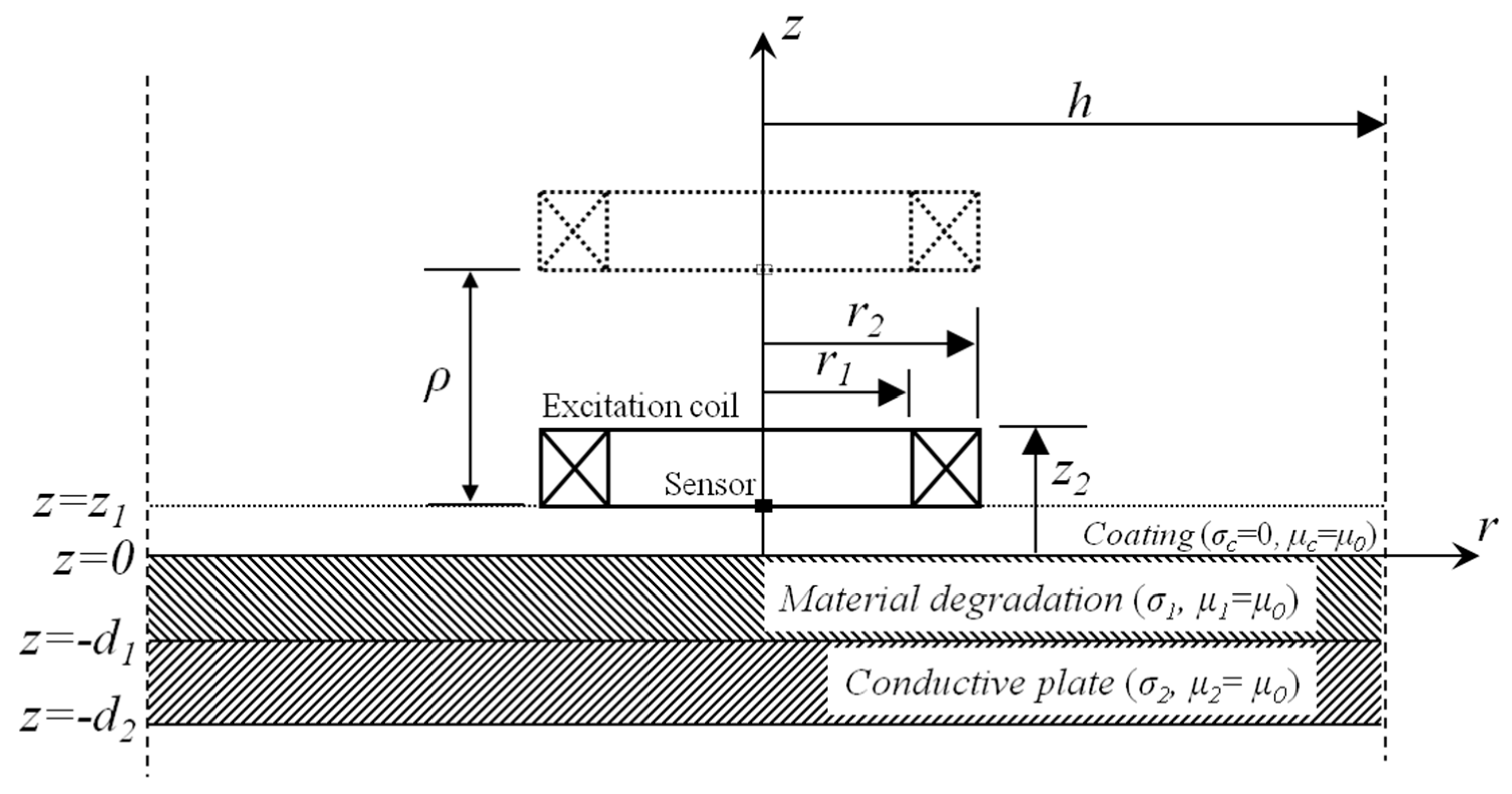
2.1. Field Formulation

The structure of the GPEC probe is similar to that of pulsed eddy current testing except that magnetic sensors deployed in the excitation coil are used for measuring gradient magnetic field in lieu of absolute magnetic field. Suppose that a cylindrical GPEC probe consisting of an excitation coil for generation of incident magnetic field and magnetic sensor for sensing the net gradient field is deployed over a coated nonmagnetic conductor with HMD. The model is shown in Figure 1. It is assumed that the length and width of the HMD area are considerably larger than the outer diameter of the excitation coil. Based on the analytical modeling [14,16], the GPEC signal concerning the z-direction gradient field of the z-component of net magnetic field is formulated as:

$$g_z\left(B_z\right)=\frac{\partial B_z}{\partial z}=\frac{{\mu }_{0}NI(t)}{H\left(r_2-r_1\right)h^2}\otimes {\displaystyle \sum _{i=1}^{\infty }{J}_0\left(a_{i}r\right)\left[e^{a_{i}z}-e^{-a_i(z+2\rho )}{\eta }_i(t)\right]\left[e^{-a_i{z}_1}-e^{-a_i{z}_2}\right]\frac{\chi \left(a_i{r}_1,a_i{r}_2\right)}{{\left[a_i{J}_0\left(a_{i}h\right)\right]}^2}}$$

(1)

where, $\otimes$ denotes convolution. H is the coil height, H = z₂ − z₁. ρ is the variation in the probe lift-off, ρ ≥ 0. I(t) and N are the excitation current and number of turns of the excitation coil. μ₀ is the permeability of vacuum. J₀ denotes the Bessel function. a_i is the positive root of J₁(a_ih) = 0. The coil coefficient χ(a_ir₁, a_ir₂) can be computed by referring to the identity in [17,18]. η_i(t) stands for the generalized temporal expression of the conductor reflection coefficient [16], and varies with HMD parameters i.e., the thickness and conductivity of HMD (d₁ and σ₁).

Equation (1) facilitates the computation of transient GPEC responses to the coated nonmagnetic conductor with HMD. By referring to the previous study revealing that LOI can only be found in the first-order derivatives of the eddy current testing signals against time [11], the first-order derivatives of the testing signals from the GPEC probe against time are further formulated. The LOI point could be identified by finding the intersection between g_z’(B_z)|_{ρ ≠ ∞} and g_z’(B_z)|_{ρ = ∞} where:

$${g_z^{\prime }\left(B_z\right)|}_{\rho \ne \infty }=\frac{{\mu }_{0}N\left\{\partial \left[I(t)\right]/\partial t\right\}}{H\left(r_2-r_1\right)h^2}\otimes {\displaystyle \sum _{i=1}^{\infty }{J}_0\left(a_{i}r\right)\left[e^{a_{i}z}-e^{-a_i(z+2\rho )}{\eta }_i(t)\right]\left[e^{-a_i{z}_1}-e^{-a_i{z}_2}\right]\frac{\chi \left(a_i{r}_1,a_i{r}_2\right)}{{\left[a_i{J}_0\left(a_{i}h\right)\right]}^2}}$$

(2)

$${g_z^{\prime }\left(B_z\right)|}_{\rho =\infty }=\frac{{\mu }_{0}N\left\{\partial \left[I(t)\right]/\partial t\right\}}{H\left(r_2-r_1\right)h^2}{\displaystyle \sum _{i=1}^{\infty }{J}_0\left(a_{i}r\right)\left[e^{a_i(z-z_1)}-e^{a_i(z-z_2)}\right]\frac{\chi \left(a_i{r}_1,a_i{r}_2\right)}{{\left[a_i{J}_0\left(a_{i}h\right)\right]}^2}}$$

(3)

M_loi and T_loi of the identified LOI point, which are invariant to ρ, can be subsequently extracted for investigation of LOI characteristics of GPEC. It is noted that GPEC probes are mostly driven by the exponential excitation current written as [19]:

$$I\left(t\right)=i_0\left(1-e^{-\frac{t}{\tau }}\right)u(t),\hspace{1em}u(t)=\{\begin{array}{l}0,\hspace{1em}t<0\\ 1,\hspace{1em}t\ge 0\end{array}$$

(4)

where, i₀ and τ denote the maximum magnitude and rising time of the excitation current, respectively whilst u(t) is Heaviside step function. For such case, Equations (2) and (3) can be individually rewritten as:

$${g_z^{\prime }\left(B_z\right)|}_{\rho \ne \infty }=\frac{{\mu }_0{i}_{0}N}{\tau H\left(r_2-r_1\right)h^2}{\displaystyle \sum _{i=1}^{\infty }{J}_0\left(a_{i}r\right)\left\{e^{a_{i}z}{e}^{-t/\tau }-e^{-a_i(z+2\rho )}\left[e^{-t/\tau }\otimes {\eta }_i(t)\right]\right\}\left[e^{-a_i{z}_1}-e^{-a_i{z}_2}\right]\frac{\chi \left(a_i{r}_1,a_i{r}_2\right)}{{\left[a_i{J}_0\left(a_{i}h\right)\right]}^2}}$$

(5)

$${g_z^{\prime }\left(B_z\right)|}_{\rho =\infty }=\frac{{\mu }_0{i}_{0}N{e}^{-t/\tau }}{\tau H\left(r_2-r_1\right)h^2}{\displaystyle \sum _{i=1}^{\infty }{J}_0\left(a_{i}r\right)e^{a_{i}z}\left(e^{-a_i{z}_1}-e^{-a_i{z}_2}\right)\frac{\chi \left(a_i{r}_1,a_i{r}_2\right)}{{\left[a_i{J}_0\left(a_{i}h\right)\right]}^2}}$$

(6)

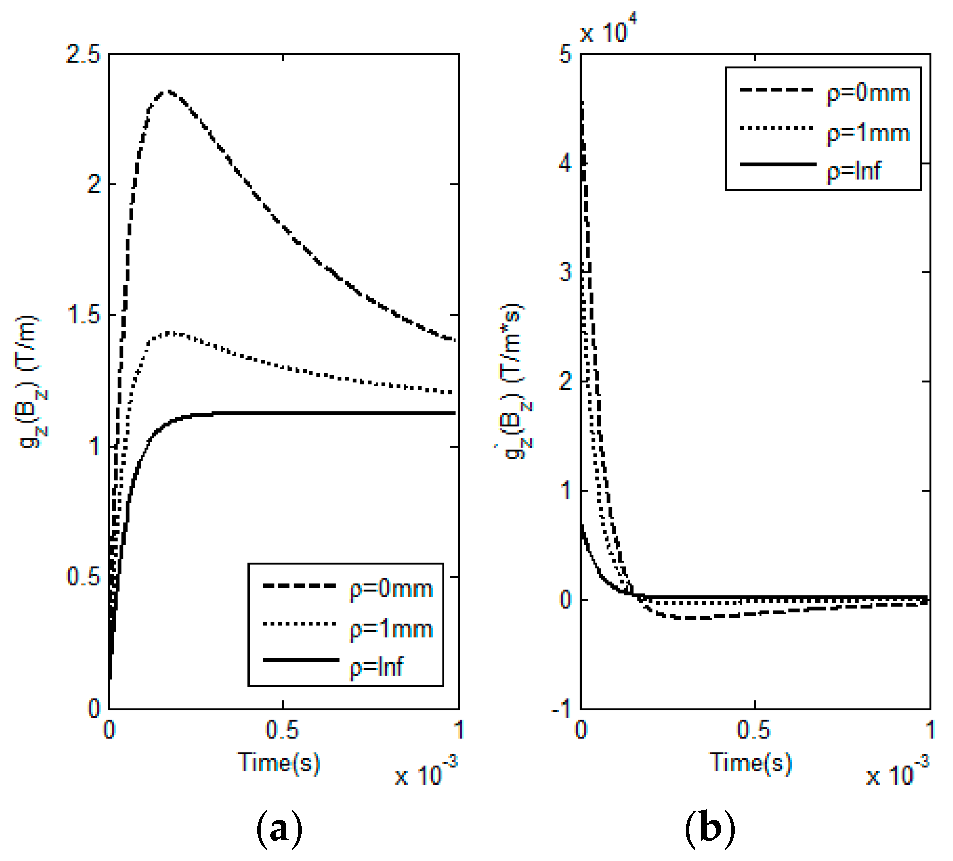
2.2. Investigation of LOI of GPEC

A series of simulations based on Equations (1)–(6) have been conducted to analyze LOI in GPEC responses to the coated nonmagnetic conductor with variable lift-offs. The correlations of M_loi and T_loi of LOI points with HMD properties are investigated. The simulation parameters are listed in

Table 1. Parameters of the excitation coil.

Coil Parameters	Value
Inner radius, r1 (mm)	11.3
Outer radius, r2 (mm)	12.5
Height, z2 − z1 (mm)	6.6
Number of turns, N	804

and

Table 2. Parameters of the sample.

Sample Parameters	Value
Thickness of the coating, z1 (mm)	0.64
Thickness of the degradation layer, d1 (mm)	0.0~3.0
Conductivity of the degradation layer, σ1 (MS/m)	25.0~34.2
Thickness of the conductor, d2 (mm)	5.0
Conductivity of the conductive plate, σ2 (MS/m)	34.2

. The fundamental frequency, duty cycle and maximum amplitude of the excitation current in rectangular waveform are 100 Hz, 50% and 0.5 A, respectively. ρ varies from 0 mm to infinity. The computed responses from the GPEC probe to the conductor with HMD (d₁ = 3 mm, σ₁ = 25 MS/m) and their first-order derivatives against time are shown in Figure 2.

It can be found from Figure 2 that for a HMD scenario the testing signals $g_z\left(B_z\right)$ from the GPEC probe with respect to different lift-off variations barely intersect, which implies that LOI doesn’t occur in GPEC signals. Whereas, the LOI point can be identified in $g_z^{\prime }\left(B_z\right)$. This agrees with the conclusion drawn from the work regarding pulsed eddy current testing [11]. Further investigation reveals that the LOI points of ${g_z^{\prime }\left(B_z\right)|}_{\rho \ne \infty }$ and ${g_z^{\prime }\left(B_z\right)|}_{\rho =\infty }$ nearly converge to one point, even though they vary with the lift-off. Compared with M_loi and T_loi of the LOI point of ${g_z^{\prime }\left(B_z\right)|}_{\rho =0}$ and ${g_z^{\prime }\left(B_z\right)|}_{\rho =\infty }$, the maximum relative errors of M_loi and T_loi of the LOI points of ${g_z^{\prime }\left(B_z\right)|}_{0<\rho \le 1mm}$ and ${g_z^{\prime }\left(B_z\right)|}_{\rho =\infty }$ are less than 0.1%. This indicates that for small ρ the LOI points of ${g_z^{\prime }\left(B_z\right)|}_{\rho \ne \infty }$ and ${g_z^{\prime }\left(B_z\right)|}_{\rho =\infty }$ are insensitive to the variation in the coating thickness because of the nature of LOI in mitigation of lift-off influence on testing signals. Therefore, two specific lift-off cases ρ = 0 and ρ = ∞ are employed in extraction of M_loi and T_loi for evaluation of HMD properties. Intensive investigation regarding relations of M_loi and T_loi with various d₁ and σ₁ of HMD are subsequently conducted. During simulations, d₁ varies from 0 mm to 3 mm with the interval of 0.3 mm whilst the variation in σ₁ is from 25 MS/m to 34.2 MS/m with the interval of 0.9 MS/m. Different combinations of d₁ and σ₁ are utilized in computation of LOI parameters via Equations (5) and (6). The simulation results are exhibited in Figure 3.

It is noticeable from Figure 3 that the LOI parameters i.e., M_loi and T_loi are dependent of the HMD properties. When the HMD thickness is fixed, T_loi is directly proportional to σ₁ whilst M_loi rises with σ₁ decreased. In contrast, when d₁ increases and σ₁ is kept constant, T_loi drops whilst M_loi increases. This indicates that by using the LOI parameters the HMD properties could be simultaneously evaluated regardless of the variation in the coating thickness.

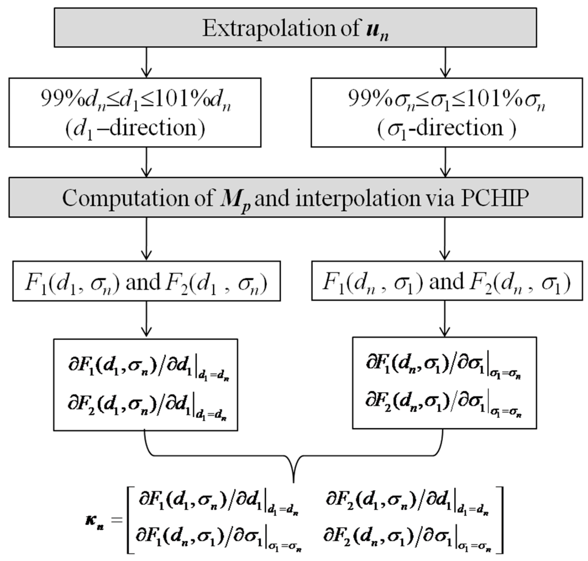
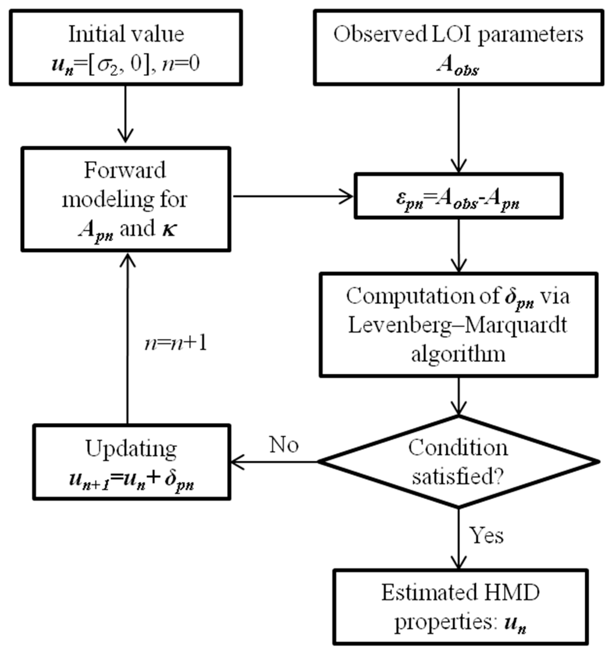
3. LOI-Based Inverse Scheme for Evaluation of HMD Properties

Let u denote the vector of the unknown HMD properties, u = [d₁, σ₁]. With other parameters known and fixed, implicit expressions depicting the relations of M_loi and T_loi with u can be established and written as:

$$M_{loi}=F_1(\mathit{u})=F_1(d_1,{\sigma }_1);\hspace{1em}{T}_{loi}=F_2(\mathit{u})=F_2(d_1,{\sigma }_1)$$

(7)

The functions F₁ and F₂ map u to the resulting amplitudes and time instants of the LOI points corresponding to different HMD properties, respectively. Suppose that u is subject to a small variation δ = [Δd₁, Δσ₁], Equation (7) is rewritten by using the Taylor series expansion as:

$$\{\begin{array}{l}{F}_1(\mathit{u}+\mathit{\delta })\approx F_1(\mathit{u})+\left[\partial F_1(\mathit{u})/\partial \mathit{u}\right]\mathit{\delta }\\ F_2(\mathit{u}+\mathit{\delta })\approx F_2(\mathit{u})+\left[\partial F_2(\mathit{u})/\partial \mathit{u}\right]\mathit{\delta }\end{array}$$

(8)

In inversion, u is iteratively pursued until the global error function depicting the deviation of the predicted LOI parameters A_p = [M_loi, T_loi] from the observation A_obs is minimized. At each iteration step, δ is sought when minimizing the quantity $\Vert {\mathit{A}}_{\mathit{obs}}-{\mathit{A}}_{\mathit{\delta }}\Vert \approx \Vert {\mathit{A}}_{\mathit{obs}}-{\mathit{A}}_{\mathit{p}}-\mathit{\kappa }\mathit{\delta }\Vert$ where, $\Vert .\Vert$denotes the norm, and κ is the 2 × 2 Jacobian matrix, κ = [∂F₁(u)/∂u, ∂F₂(u)/∂u]^T.

It is noted that during iteration A_p can be readily computed by using the analytical-modeling based algorithm elaborated in Section 2.1. Compared with the computation of A_p, it is formidable to directly calculate the Jacobian matrix κ. In light of this, indirect computation based on interpolation is adopted, whose schematic illustration is shown in Figure 4. At each iteration step, besides the calculation of A_pn with an updated u_n (n denoting the iteration number), u_n is firstly extrapolated in the d₁-direction (99% d_n ≤ d₁ ≤ 101% d_n whilst σ₁ is fixed at σ_n). The number of samples is 201. The resulting LOI parameters corresponding to defined samples are computed, and subsequently interpolated by using the Piecewise Cubic Hermite Interpolating Polynomial (PCHIP) in an effort to derive F₁(d₁, σ_n) and F₂(d₁, σ_n). The differentiation of F₁(d₁, σ_n) and F₂(d₁, σ_n) can be readily realized by using the routine ‘fnder’ in Matlab. ${\partial F_1(d_1,{\sigma }_n)/\partial d_1|}_{d_1=d_n}$ and ${\partial F_2(d_1,{\sigma }_n)/\partial d_1|}_{d_1=d_n}$ of κ_n are thus derived from evaluation of PCHIP-based functions $\partial F_1(d_1,{\sigma }_n)/\partial d_1$ and $\partial F_2(d_1,{\sigma }_n)/\partial d_1$ with d₁ = d_n. The computation of ${\partial F_1(d_n,{\sigma }_1)/\partial {\sigma }_1|}_{{\sigma }_1={\sigma }_n}$ and ${\partial F_2(d_n,{\sigma }_1)/\partial {\sigma }_1|}_{{\sigma }_1={\sigma }_n}$ is similar to that for ${\partial F_1(d_1,{\sigma }_n)/\partial d_1|}_{d_1=d_n}$ and ${\partial F_2(d_1,{\sigma }_n)/\partial d_1|}_{d_1=d_n}$ except for the extrapolation of u_n in the σ₁-direction (99% σ_n ≤ σ₁ ≤ 101% σ_n whilst d₁ is fixed at d_n). With A_p and κ computed, Levenberg–Marquardt algorithm is employed to calculate δ for updating u. The LOI-based inversion terminates when the general conditions of Levenberg–Marquardt algorithm are met [18]. The schematic illustration of the proposed inverse scheme is presented in Figure 5. Note that the initial guess regarding u is referred to the HMD-free case where σ₁ = σ₂ and d₁ = 0 mm. It should be pointed out that: (1) thanks to the analytical model utilized in inversion the proposed inverse scheme is efficient in iteratively seeking the solutions to unknown HMD properties; but (2) it can hardly be applied to evaluation of properties of the localized HMD whose size is smaller than the excitation coil in the GPEC probe.

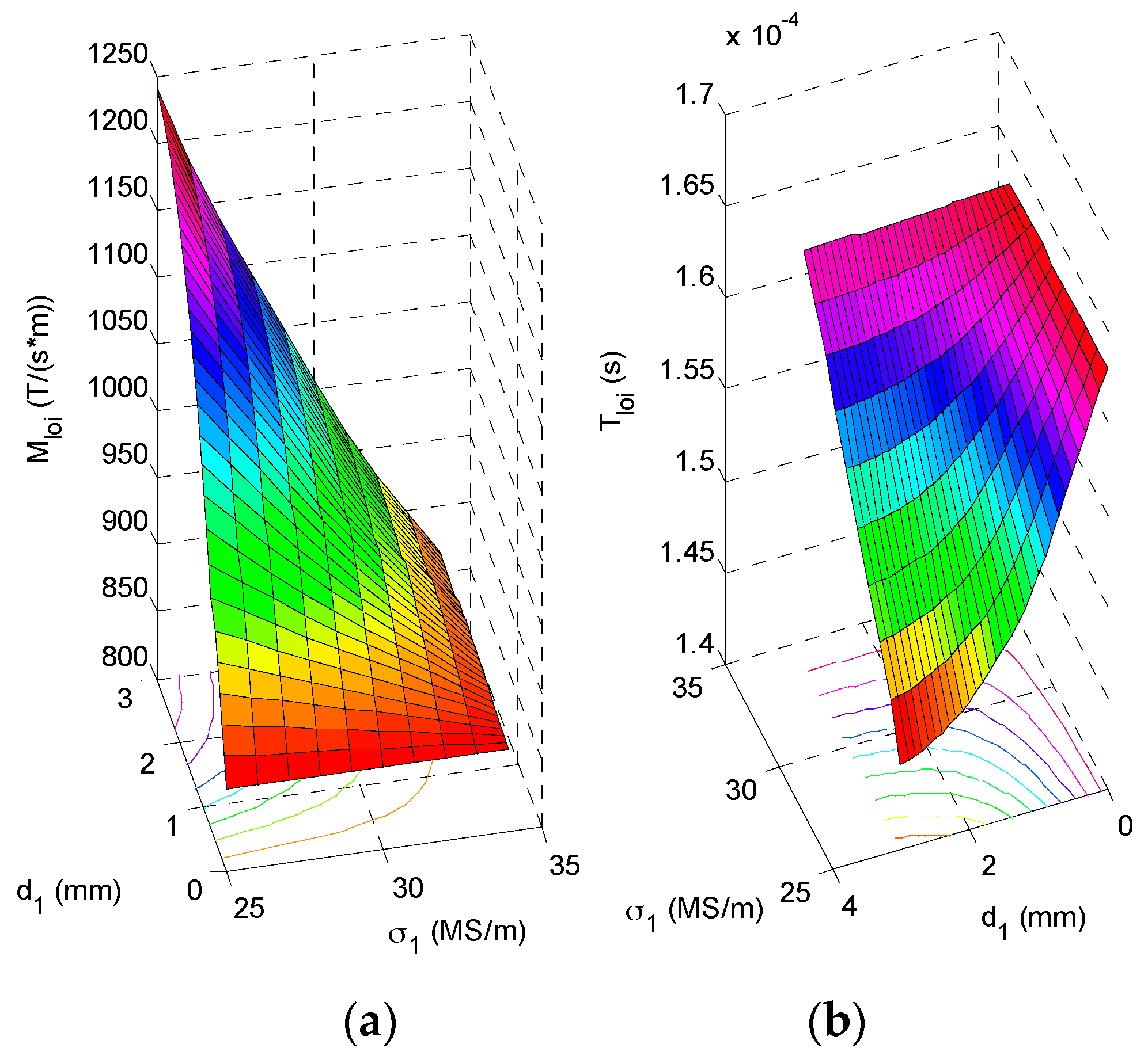
4. Corroboration via Finite Element Modeling

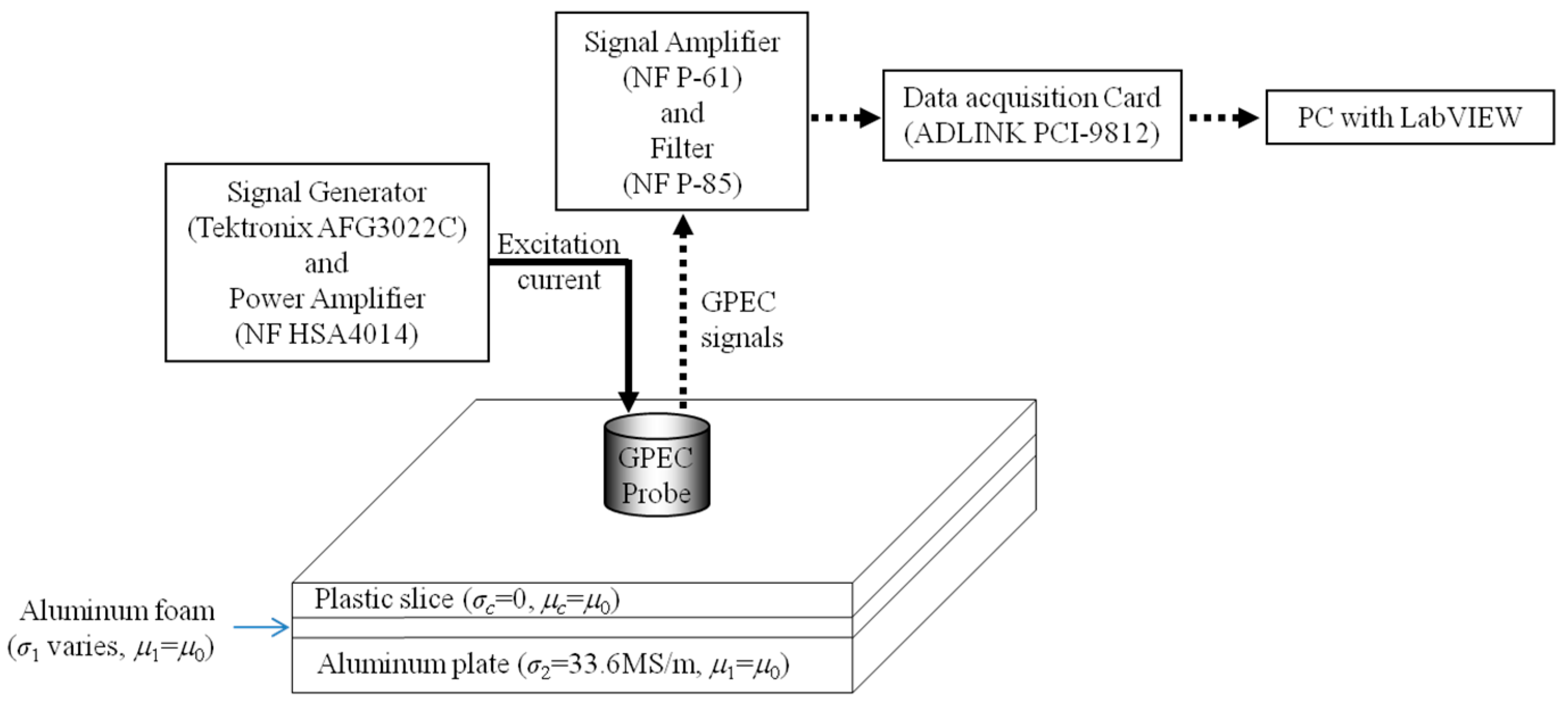
The proposed LOI-based inverse scheme is verified via finite element modeling [20,21] which gives the simulated observation corresponding to a HMD scenario with u = [1.6 mm, 28.5 MS/m]. The other model parameters are same as those listed in Table 1 and Table 2. The excitation current I(t) is exhibited in Figure 6. The acquired signals and their first-order derivatives from finite element modeling regarding GPEC are shown in Figure 7. The LOI point identified by finding the intersection point of the first-order derivative of the acquired signal with ρ = 0 against time and that with ρ = ∞. Following this, the LOI parameters are extracted and taken as the observation A_obs = [244.4 T/m·s, 171.1 μs].

The observation obtained from finite element modeling and initial guess regarding u are input into the proposed inversion in an attempt to inversely retrieve the conductivity and thickness of the predefined HMD. The estimated properties of the HMD (u_est) and their comparison with the true values (u_true) are presented in

Table 3. Comparison between approximated HMD properties and true values against different SNRs of the excitation current signals.

SNR	Inf *	26 dB	20 dB	14 dB
utrue	[1.60 mm, 28.50 MS/m]
uest	[1.63 mm, 29.05 MS/m]	[1.54 mm, 27.19 MS/m]	[1.68 mm, 26.83 MS/m]	[1.49 mm, 26.42 MS/m]
Relative error	[1.7%, 1.9%]	[3.8%, 4.6%]	[5.1%, 5.8%]	[6.9%, 7.3%]

* “Inf” denotes SNR is infinite. In such case, the excitation current signal is free of the noise.

. It is noted that in a bid to evaluate the robustness of the proposed inverse scheme, the excitation current signals with different Signal-to-Noise Ratios (SNRs) are used in finite element modeling, and thus the observed LOI parameters are polluted due to the random noise introduced to the noise-free excitation current signal. Note that: (1) the ratio of the random noise amplitude to the magnitude of the noise-free excitation current signal varies from 0% to 20%; (2) the excitation current signals with different SNRs are derived from superposition of the random noise signals and noise-free excitation current signal; and (3) I(t) used in the forward modeling regarding computation of A_p and κ during inversion is free of noise.

It can be seen from Table 3 that the approximated HMD properties have good agreement with the true values even though the signals are subject to noises. This implies the potential of the GPEC probe along with the LOI-based inverse scheme in simultaneous evaluation of properties of HMD in coated conductors. It is also noticeable from Table 3 that with the noise amplitude increased, the estimation accuracy of the proposed inverse scheme decreases. This indicates that before the extraction of the observed LOI parameters, proper low-pass filtering should be employed in the signal processing regarding acquired field signals in order to cancel out the extraneous noise. Further analysis of the results listed in Table 3 reveals that the accuracy in estimation of the HMD thickness is higher than that for the HMD conductivity. The reasoning could lie in the fact that the absolute value of the HMD conductivity is considerably larger than that of the HMD thickness. During inversion, the resolution of the space where the solution to an unknown HMD conductivity is sought is less than that of the solution space regarding the HMD thickness. Based on the verification via finite element modeling, the feasibility of the GPEC probe with the proposed inverse scheme in HMD evaluation is further investigated through experiments.

5. Experiments

A GPEC system has been built up in order to further evaluate the applicability of the GPEC probe together with the proposed inverse scheme in simultaneous assessment of properties of HMD in a coated Aluminum plate. The system setup is shown in Figure 8. The parameters of the excitation coil of the GPEC probe are same as those listed in Table 1. The pulse repetition frequency, duty cycle, maximum amplitude and rising time of the excitation current driving the excitation coil are 100 Hz, 50%, 0.3 A and 62.7 μs (measured from the acquired signal of the excitation current), respectively. A tunnel magneto-resistance sensor (MultiDimension TMR-4002, MultiDimension Technology Co., Ltd., Zhangjiagang Free Trade Zone, China) is used to sense the z-direction gradient field of the z-component of net magnetic field, and deployed at the bottom centre of the excitation coil.

In an attempt to simulate the coated Aluminum plate with HMD, three stratified planar structures in 100 mm × 100 mm (length × width) are fabricated and taken as the specimens under evaluation. Each specimen has three layers: a plastic slice as the nonconductive protection coating; a slab of Aluminum foam as the layer of material degradation; and an Aluminum plate as the rest of the conductive region free of material degradation. Besides the specimen parameters exhibited in Figure 8, the other parameters of each specimen are listed in

Table 4. Parameters of the specimens.

	#1	#2	#3
Thickness of the plastic slice, z1 (mm)	0.2	0.5	0.2
Thickness of the Aluminum foam, d1 (mm)	0.9	1.5	1.8
Conductivity of the Aluminum foam, σ1 (MS/m)	32.3	25.9	21.2
Thickness of the Aluminum block, d2 − d1 (mm)	4.1	3.5	3.2

. It is noted the Aluminum foams with different conductivities lower than that of the Aluminum block (σ₂ = 33.6 MS/m) are realized by setting different porosity densities during fabrication. Their apparent conductivities are measured by using direct current potential drop method [22,23,24,25]. A standard Aluminum sample with the conductivity and dimension of 33.6 MS/m and 300 mm × 300 mm × 5 mm (length × width × thickness), respectively is used to calibrate the system and sensor to cancel out the deviation of measured M_loi and T_loi against predicted values.

Prior to the experiment with samples, the GPEC probe is firstly deployed in the air to acquire the signal of g_z(B_z)|_{ρ = ∞}. g_z’(B_z)|_{ρ = ∞} is subsequently computed by taking the first-order derivative of g_z(B_z)|_{ρ = ∞} against time. Following this, g_z’(B_z)|_{ρ ≠ ∞} for each specimen is obtained via differentiation of the acquired signal of g_z(B_z)|_{ρ ≠ ∞} against time when the probe is placed over each specimen. The experimental signals against different specimens are exhibited in Figure 9. The observed LOI parameters with respect to every specimen are subsequently acquired by extracting the amplitude and time instant corresponding to the intersection point of g_z’(B_z)|_{ρ ≠ ∞} and g_z’(B_z)|_{ρ = ∞}: 150.3 T/m·s and 198.8 μs for Specimen #1; 192.0 T/m·s and 183.4 μs for Specimen #2; 192.0 T/m·s and 181.0 μs for Specimen #3.

The observed values are input into inversion for approximation of HMD properties of each specimen. The estimated results regarding the thickness and conductivity of simulated degradation for each specimen and their comparison with the true values are tabulated in

Table 5. Comparison of estimated HMD properties u_est with the true values u_true.

	Specimen #1	Specimen #2	Specimen #3
utrue	[0.9 mm, 32.3 MS/m]	[1.5 mm, 25.9 MS/m]	[1.8 mm, 21.2 MS/m]
uest	[0.86 mm, 30.63 MS/m]	[1.42 mm, 28.05 MS/m]	[1.87 mm, 19.89 MS/m]
Relative error	[4.4%, 5.2%]	[5.3%, 8.3%]	[3.9%, 6.2%]

.

It can be found from Table 5 that the estimated results have good agreement with the true values of the Aluminum foam simulating the material degradation with the relative error less than 9.0%. It is noted that thanks to the characteristics of LOI, for each specimen M_loi and T_loi is insensitive to thickness variation of the plastic slice. For example, regarding Specimen #1 with the coating thicknesses of 0 mm and 0.5 mm, M_loi and T_loi agree well with those for the original specimen setup with relative error less than 1.0%. The averaged total inversion time is 5.3 s with the number of iteration steps of 23. It can be seen from the experimental investigation that the GPEC probe in conjunction with the LOI-based inverse scheme is applicable to simultaneous evaluation of properties of HMD in coated nonmagnetic conductors. This benefits the real-time monitoring of HMD in in-service coated conductive structures.

6. Concluding Remarks

In this paper, GPEC probes for evaluation of properties of material degradation hidden in coated conductive structures are intensively investigated through theoretical simulations and experiments. Closed-form expressions of GPEC responses to conductors with HMD are formulated based on the analytical modeling. A series of simulations of GPEC have been carried out for analysis of LOI characteristics and correlations between LOI parameters and HMD properties. It has been found from simulation results that LOI can only be found in the first-order derivative of the GPEC signal against time. The LOI parameters, M_loi and T_loi have close correlations with the HMD properties. Therefore, a fast inverse scheme based on LOI in signals from the GPEC probe is proposed for simultaneous assessment of the conductivity and thickness of HMD in planar nonmagnetic conductors. The proposed inverse method is subsequently verified by finite element modeling and experiments which give the simulated observation corresponding to the predefined HMD properties. The comparison of the estimated HMD properties and true values has revealed that the GPEC probe along with the proposed LOI-based inverse scheme is applicable for quantitatively evaluating properties of HMD in coated conductive structures without much loss in accuracy.

In light of the technical merits of GPEC and LOI, the advantages of the proposed probe with the inverse scheme include: (1) evaluation of HMD properties regardless of small variation in the coating thickness; and (2) efficient estimation of HMD properties with high accuracy. Whereas, it should be noted that the application of the proposed technique is barely applicable to evaluation of the localized HMD whose size is smaller than the excitation coil in the probe. This opens up further work focusing on the simultaneous assessment of properties of localized HMD in coated conductive structures.

References

1. Calabrese, L.; Proverbio, E.; Galtieri, G.; Borsellino, C. Effect of Corrosion Degradation on Failure Mechanisms of Aluminium/steel Clinched Joints. Mater. Des. 2015, 87, 473–481. [Google Scholar] [CrossRef]
2. Javier, M.; Jaime, G.; Ernesto, S. Non-Destructive Techniques Based on Eddy Current Testing. Sensors 2011, 11, 2525–2565. [Google Scholar] [CrossRef]
3. Zhou, D.Q.; Li, Y.; Yan, X.; You, L.; Zhang, Q.; Liu, X.B.; Qi, Y. The Investigation on The Optimal Design of Rectangular PECT Probes for Evaluation of Defects in Conductive Structures. Int. J. Appl. Electromagn. Mech. 2013, 42, 319–326. [Google Scholar]
4. Li, Y.; Yan, B.; Li, D.; Li, Y.L.; Zhou, D.Q. Gradient-field Pulsed Eddy Current Probes for Imaging of Hidden Corrosion in Conductive Structures. Sens. Actuators A Phys. 2016, 238, 251–265. [Google Scholar] [CrossRef]
5. Mandache, C.; Lefebvre, J. Transient and Harmonic Eddy Currents: Lift-off Point of Intersection. NDT & E Int. 2006, 39, 57–60. [Google Scholar]
6. Fan, M.B.; Cao, B.H.; Yang, P.P.; Li, W.; Tian, G.Y. Elimination of Liftoff Effect Using a Model-based Method for Eddy Current Characterization of a Plate. NDT E Int. 2015, 74, 66–71. [Google Scholar] [CrossRef]
7. Li, Y.; Chen, Z.M.; Qi, Y. Generalized Analytical Expressions of Liftoff Intersection in PEC and a Liftoff-intersection-based Fast Inverse Model. IEEE Trans. Magn. 2011, 47, 2931–2934. [Google Scholar] [CrossRef]
8. Fan, M.B.; Cao, B.H.; Tian, G.Y.; Ye, B.; Li, W. Thickness Measurement Using Liftoff Point of Intersection in Pulsed Eddy Current Responses for Elimination of Liftoff Effect. Sens. Actuators A Phys. 2016, 251, 66–74. [Google Scholar] [CrossRef]
9. Giguere, J.; Dubois, J. Pulsed Eddy Current: Finding Corrosion Independently of Transducer Lift-off. AIP Conf. Proc. 2000, 509, 449–456. [Google Scholar]
10. Giguere, J.; Lepine, A.; Dubois, J. Detection of Cracks Beneath Rivets via Pulsed Eddy Current Technique. AIP Conf. Proc. 2002, 21, 1968–1975. [Google Scholar]
11. Tian, G.Y.; Li, Y.; Mandache, C. Study of Lift-off Invariance for Pulsed Eddy-Current Signals. IEEE Trans. Magn. 2009, 45, 184–191. [Google Scholar] [CrossRef]
12. Xie, S.J.; Chen, Z.M.; Takagi, T.; Uchimoto, T. Quantitative Non-destructive Evaluation of Wall Thinning Defect in Double-layer Pipe of Nuclear Power Plants Using Pulsed ECT Method. NDT E Int. 2015, 75, 87–95. [Google Scholar] [CrossRef]
13. Bai, B.; Tian, Y.; Simm, A.; Tian, L.; Cheng, H. Fast Crack Profile Reconstruction Using Pulsed Eddy Current Signals. NDT E Int. 2013, 54, 37–44. [Google Scholar] [CrossRef]
14. Li, Y.; Tian, G.Y.; Simm, A. Fast Analytical Modelling for Pulsed Eddy Current Evaluation. NDT E Int. 2008, 41, 477–483. [Google Scholar] [CrossRef]
15. Madsen, K.; Nielsen, H.B.; Tingleff, O. Methods for Nonlinear Least Squares Problems. Soc. Ind. Appl. Math. 2012, 1, 1409–1415. [Google Scholar]
16. Li, Y.; Yan, B.; Li, D.; Jing, H.Q.; Li, Y.L.; Chen, Z.M. Pulse-modulation Eddy Current Inspection of Subsurface Corrosion in Conductive Structures. NDT E Int. 2016, 79, 142–149. [Google Scholar] [CrossRef]
17. Li, Y.; Yan, B.; Li, W.J.; Li, D. Thickness Assessment of Thermal Barrier Coatings of Aeroengine Blades via Dual-frequency Eddy Current Evaluation. IEEE Magn. Lett. 2016, 7, 1304905. [Google Scholar] [CrossRef]
18. Li, Y.; Chen, Z.M.; Mao, Y.; Qi, Y. Quantitative Evaluation of Thermal Barrier Coating Based on Eddy Current Technique. NDT E Int. 2012, 50, 29–35. [Google Scholar]
19. Bowler, J.; Johnson, M. Pulsed Eddy-current Response to a Conducting Half-space. IEEE Trans. Magn. 1997, 33, 2258–2264. [Google Scholar] [CrossRef]
20. Rosell, A. Efficient Finite Element Modeling of Eddy Current Probability of Detection with Transmitter–Receiver Sensors. NDT E Int. 2015, 75, 48–56. [Google Scholar] [CrossRef]
21. Rosell, A.; Persson, G. Finite Element Modeling of Closed Cracks in Eddy Current Testing. Int. J. Fatigue 2012, 41, 30–38. [Google Scholar] [CrossRef]
22. Wang, X.; Xie, S.J.; Li, Y.; Chen, Z.M. Efficient Numerical Simulation of DC Potential Drop Signals for Application to Metallic Foam. COMPEL: Int. J. Comp. Math. Electr. Electron. Eng. 2014, 3, 147–156. [Google Scholar] [CrossRef]
23. Zhang, J.; Xie, J.; Wang, J.; Li, Y.; Chen, M. Quantitative Non-destructive Testing of Metallic Foam Based on Direct Current Potential Drop Method. IEEE Trans. Magn. 2012, 48, 375–378. [Google Scholar] [CrossRef]
24. Brinnel, V.; Dobereiner, B.; Munstermann, S. Characterizing Ductile Damage and Failure: Application of the Direct Current Potential Drop Method to Uncracked Tensile Specimens. Procedia Mater. Sci. 2014, 3, 1161–1166. [Google Scholar] [CrossRef]
25. Ali, M.R.; Saka, M.; Tohmyoh, H. A Time-dependent Direct Current Potential Drop Method to Evaluate Thickness of an Oxide Layer Formed Naturally and Thermally on a Large surface of Carbon Steel. Thin Solid Films 2012, 525, 77–83. [Google Scholar] [CrossRef]
Figure 1. 2D axi-symmetric model of a GPEC probe over a coated nonmagnetic conductor with HMD.
Sensors 17 00943 g001
Figure 2. Predicted GPEC responses to the sample and their first-order derivatives against time. (a) GPEC signals against different lift-offs; (b) first-order derivatives of the GPEC signals.
Sensors 17 00943 g002
Figure 3. Correlations of (a) Mloi and (b) Tloi with d1 and σ1 of HMD.
Sensors 17 00943 g003
Figure 4. Schematic illustration of the computation of κ.
Sensors 17 00943 g004
Figure 5. Schematic illustration of the proposed inverse scheme.
Sensors 17 00943 g005
Figure 6. Excitation current I(t).
Sensors 17 00943 g006
Figure 7. Simulated GPEC signals and their first-order derivatives against time. (a) GPEC signals; (b) first-order derivatives of the GPEC signals.
Sensors 17 00943 g007
Figure 8. Schematic illustration of the inspection system and specimen.
Sensors 17 00943 g008
Figure 9. Measured GPEC signals and their first-order derivatives against time. (a) GPEC signals acquired in experiments; (b) first-order derivatives of the GPEC signals (250 μs ≥ t ≥ 150 μs).
Sensors 17 00943 g009