
Adaptive Data Aggregation and Compression to Improve Energy Utilization in Solar-Powered Wireless Sensor Networks


Abstract
:1. Introduction
2. Related Work
2.1. Data Aggregation in WSNs
2.2. Data Compression in WSNs
2.3. Energy Utilization in WSNs
3. Adaptive Aggregation and Compression Scheme
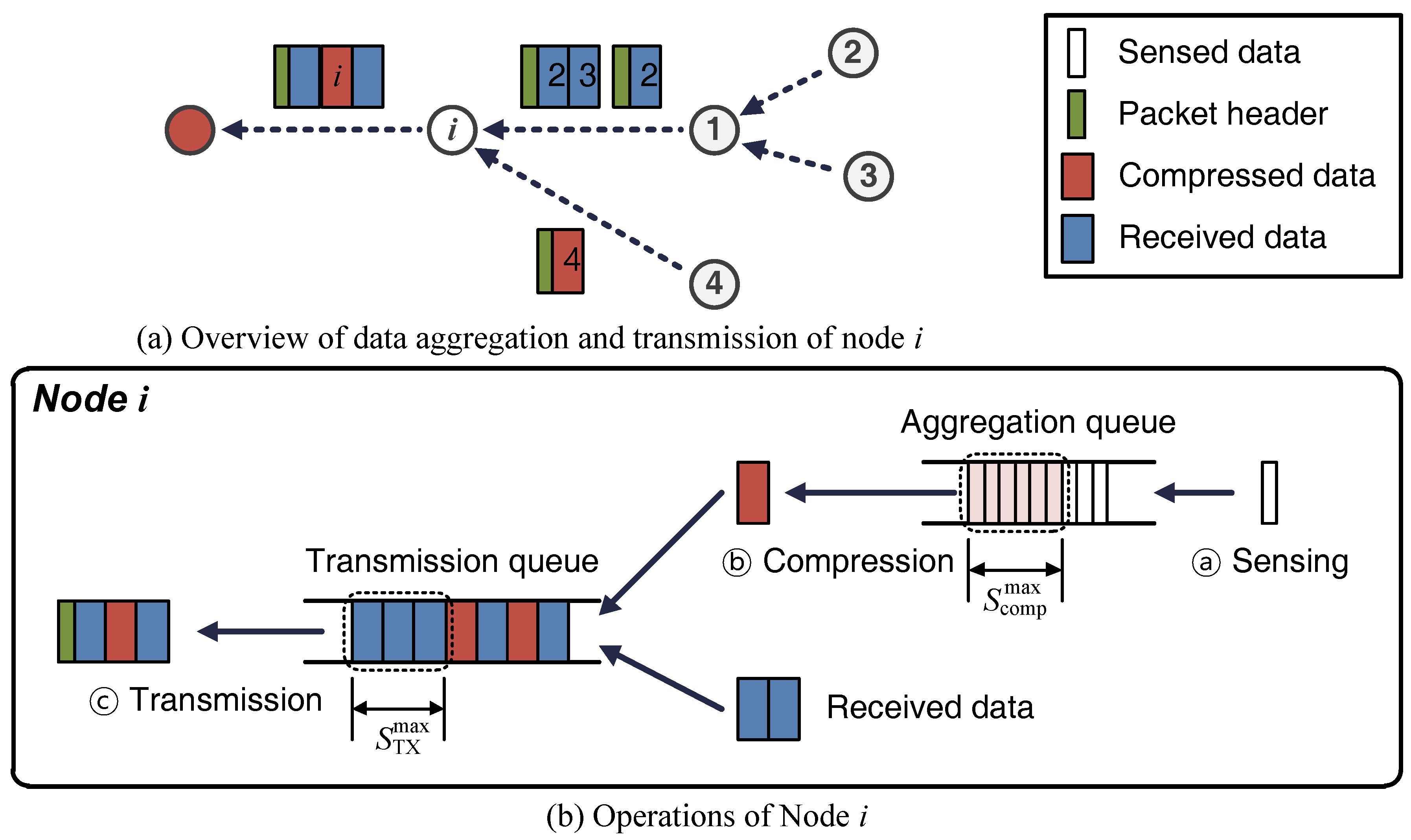
3.1. Sensor Node Operations
Sensing
Compression
Transmission
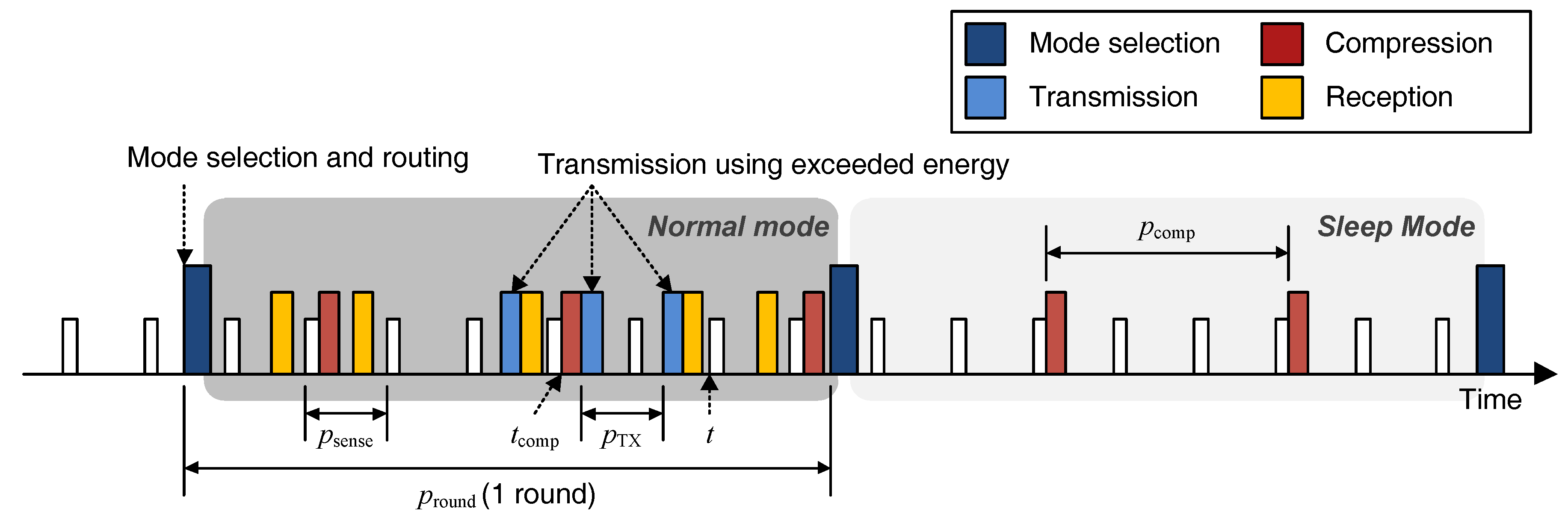
Mode selection
- Normal mode is selected when there is sufficient energy to continue sensing, compression, and transmission during the next round.
- Sleep mode is selected if the residual energy would otherwise run out during the next round. In this mode, a node only performs sensing and compression. It turns off its wireless module, and thus any data sent to it during the subsequent period is lost . To avoid this happening, nodes select their modes before the routing process, which excludes nodes in sleep mode.
3.2. Mode Selection
3.3. Choosing Whether to Transmit Data
4. Performance Evaluation
4.1. Simulation
4.2. Simulation Results
4.2.1. Residual Energy and Blackout Nodes
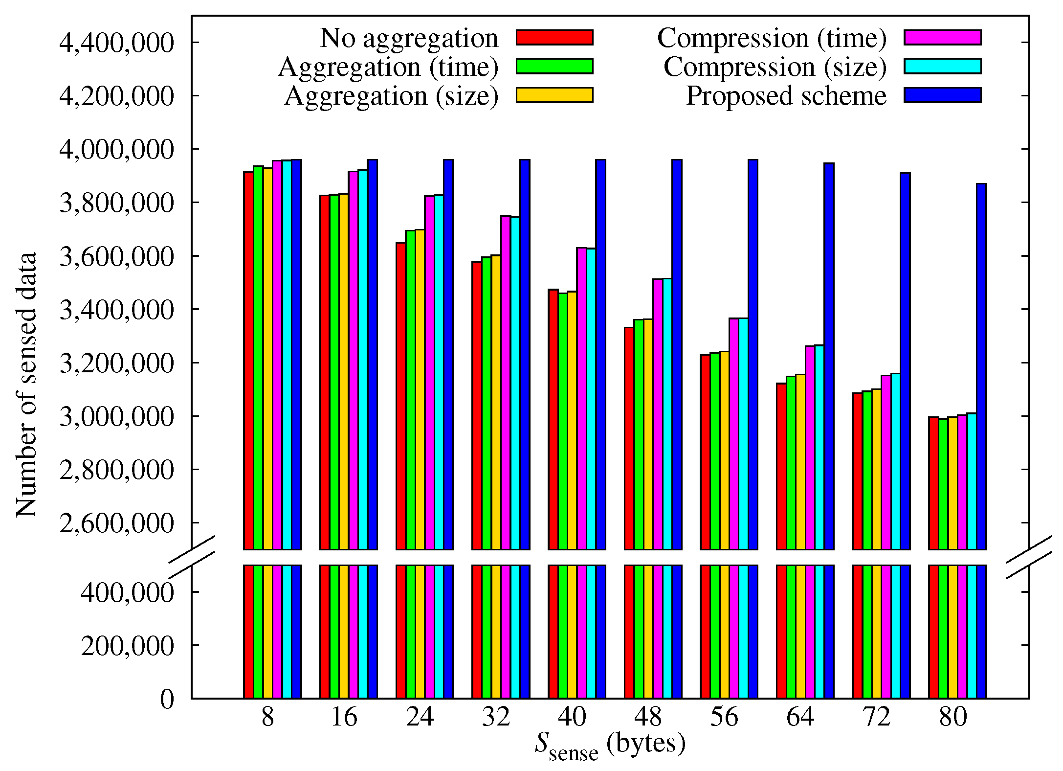
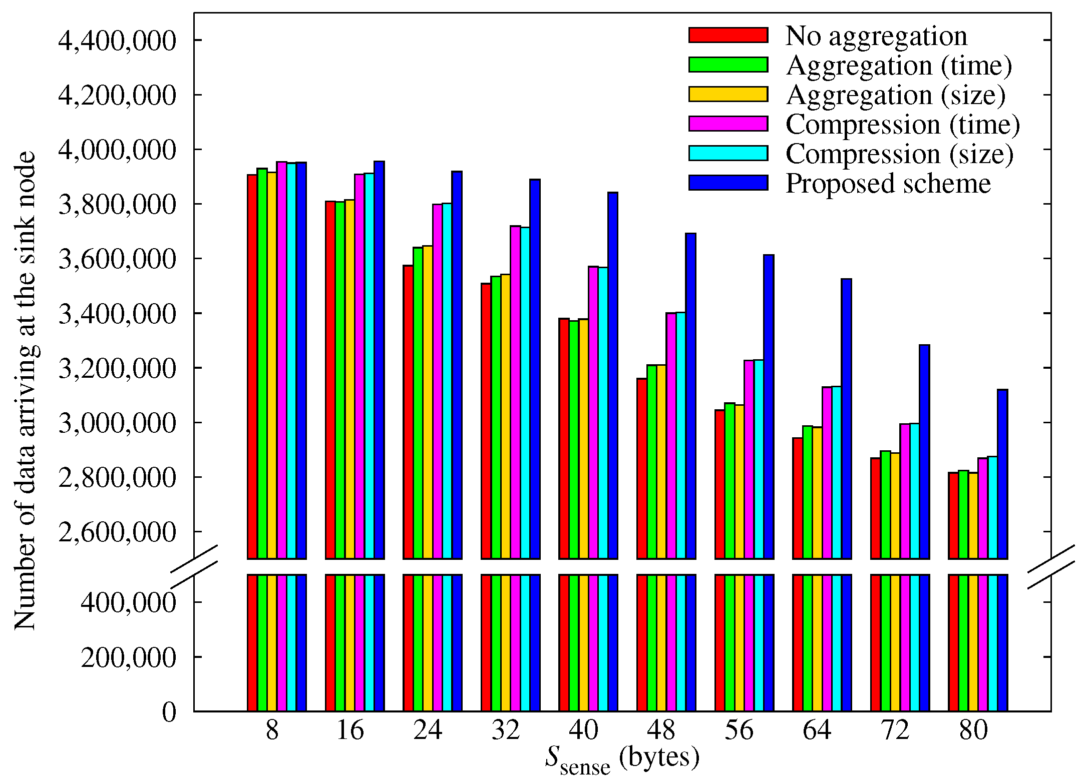
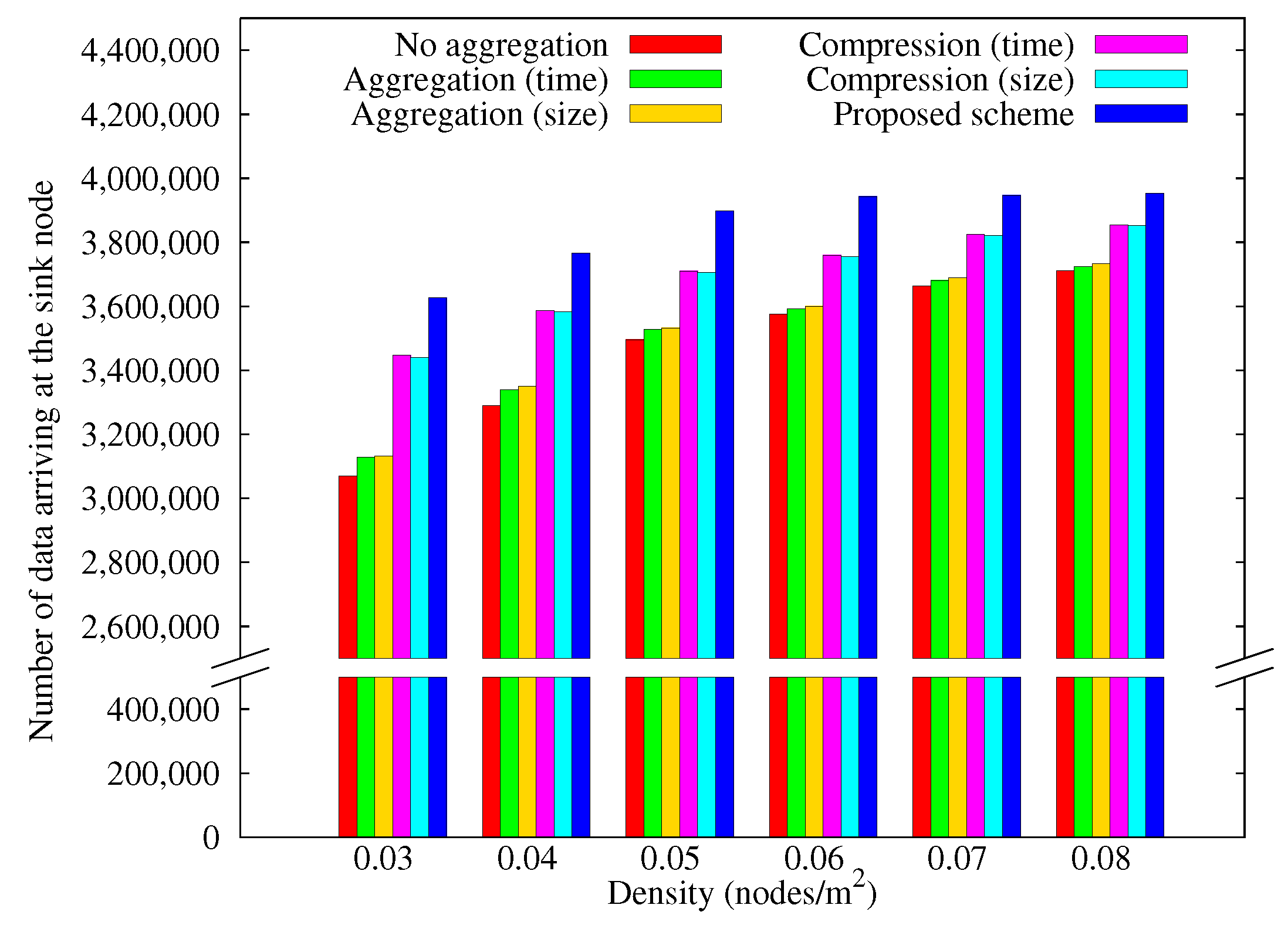
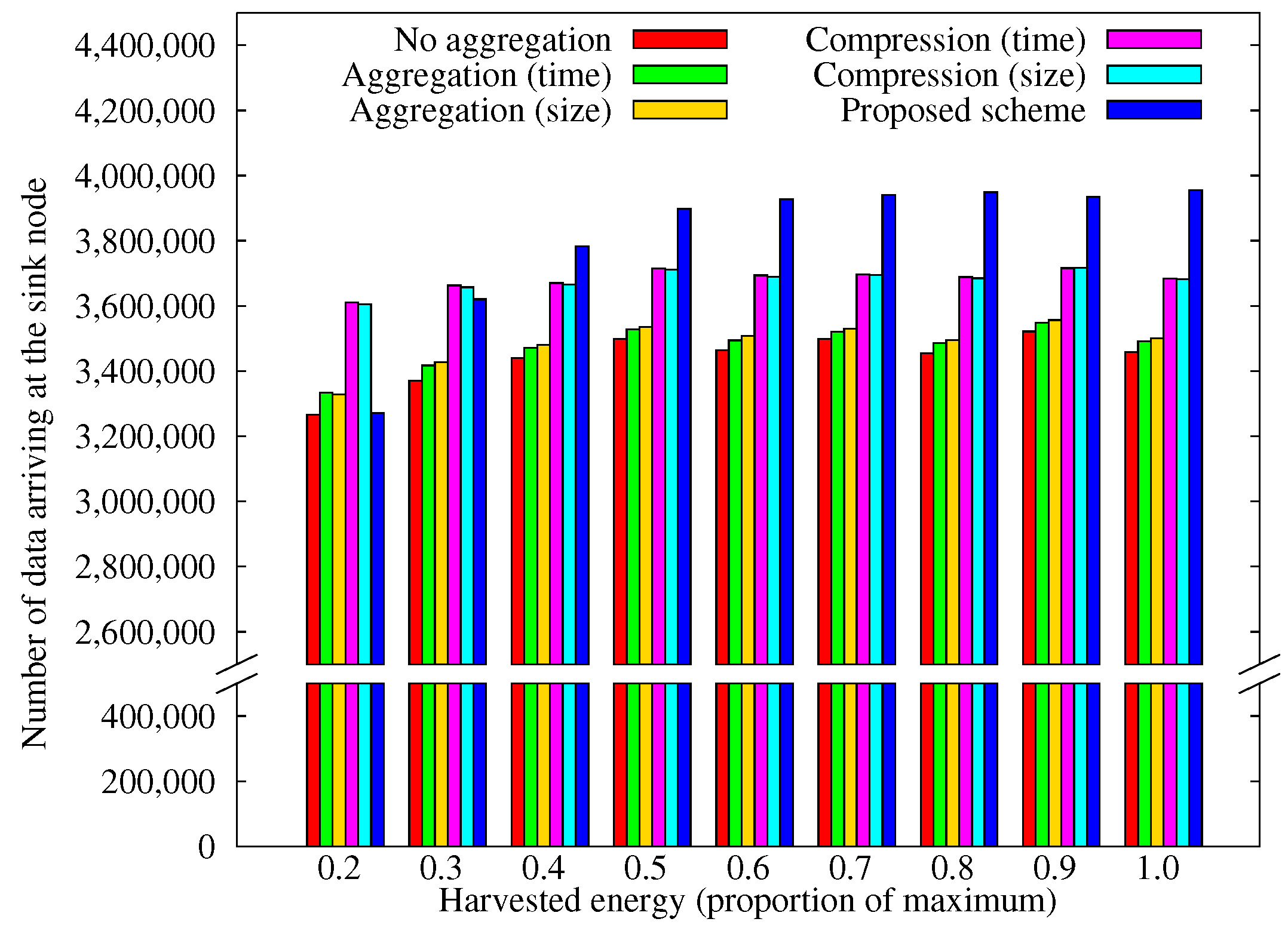
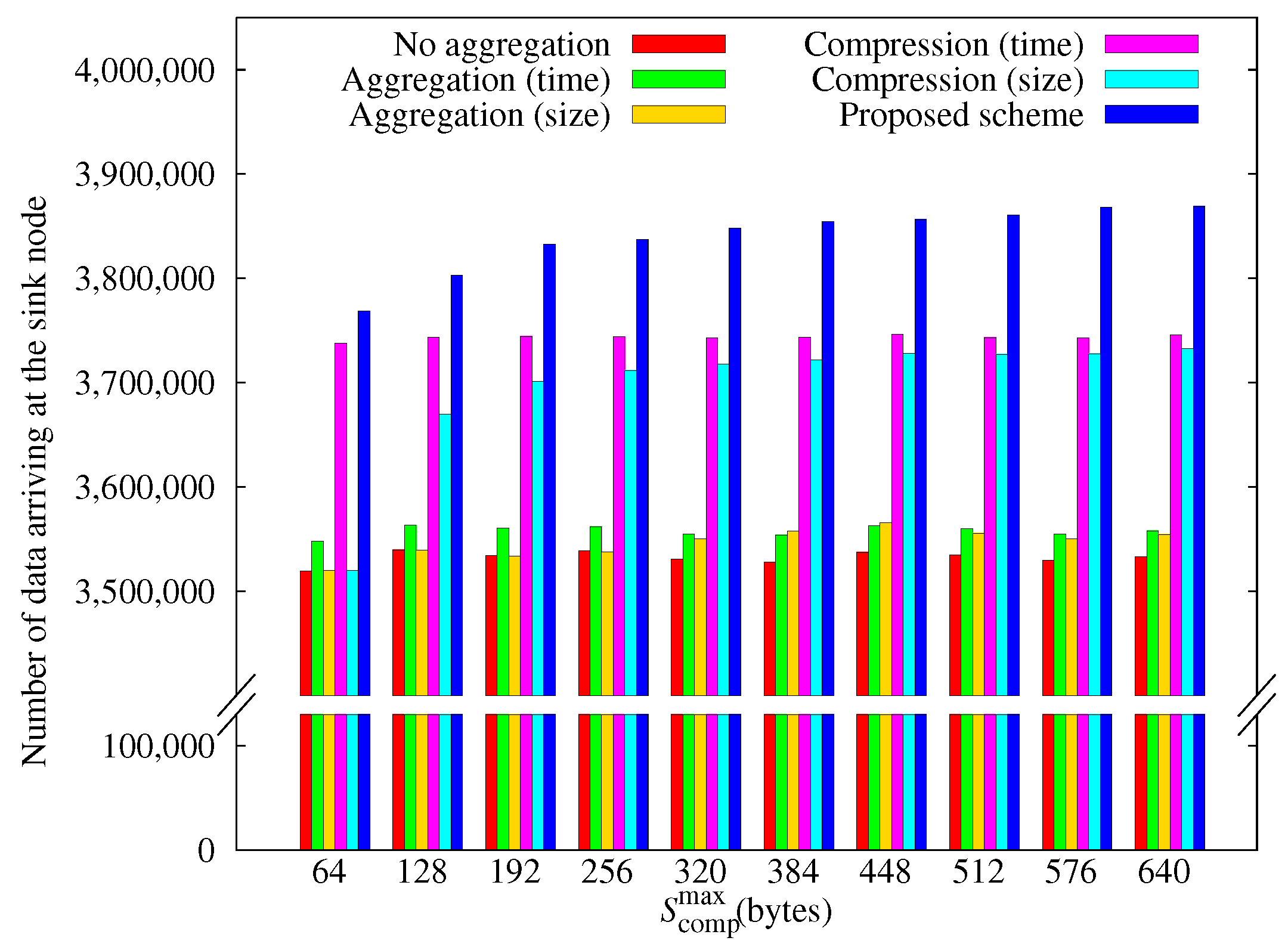
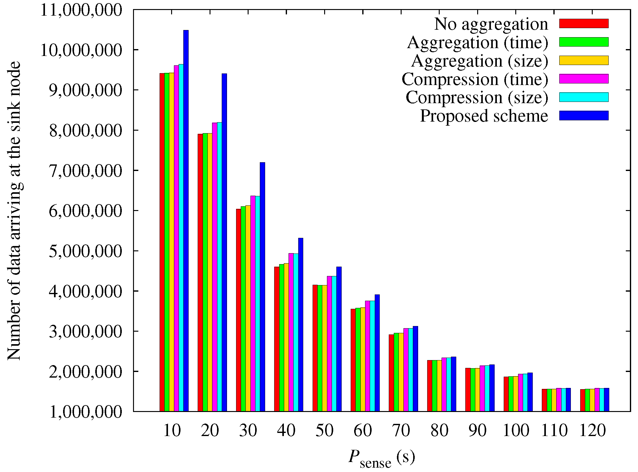
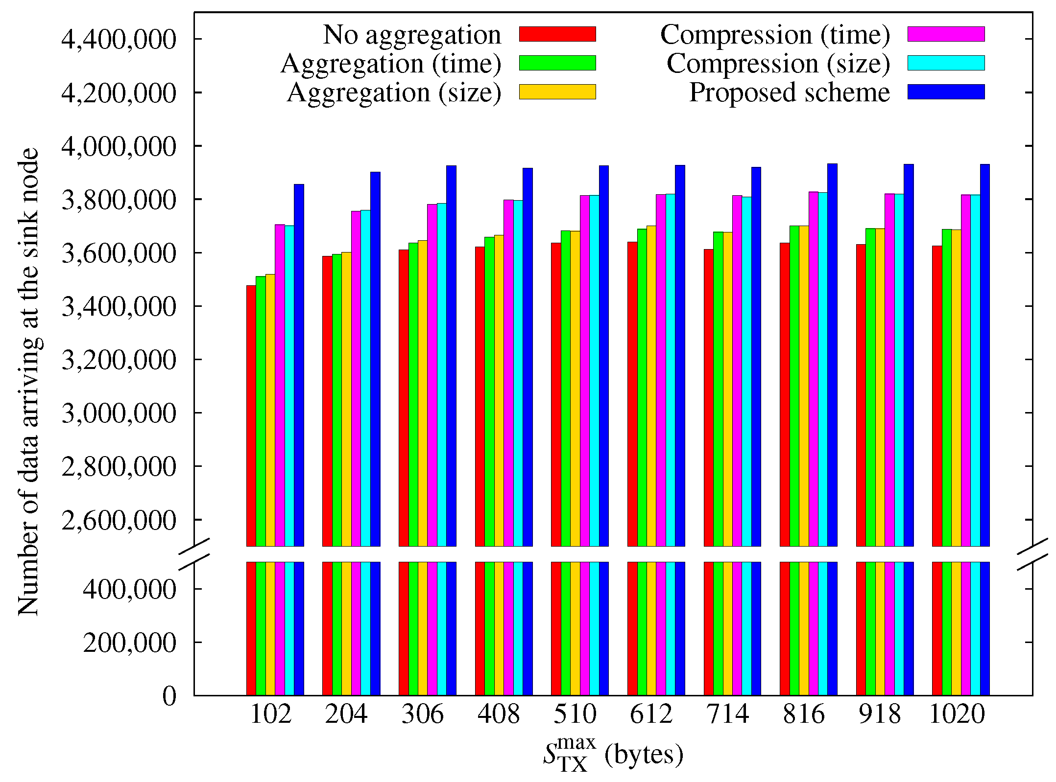
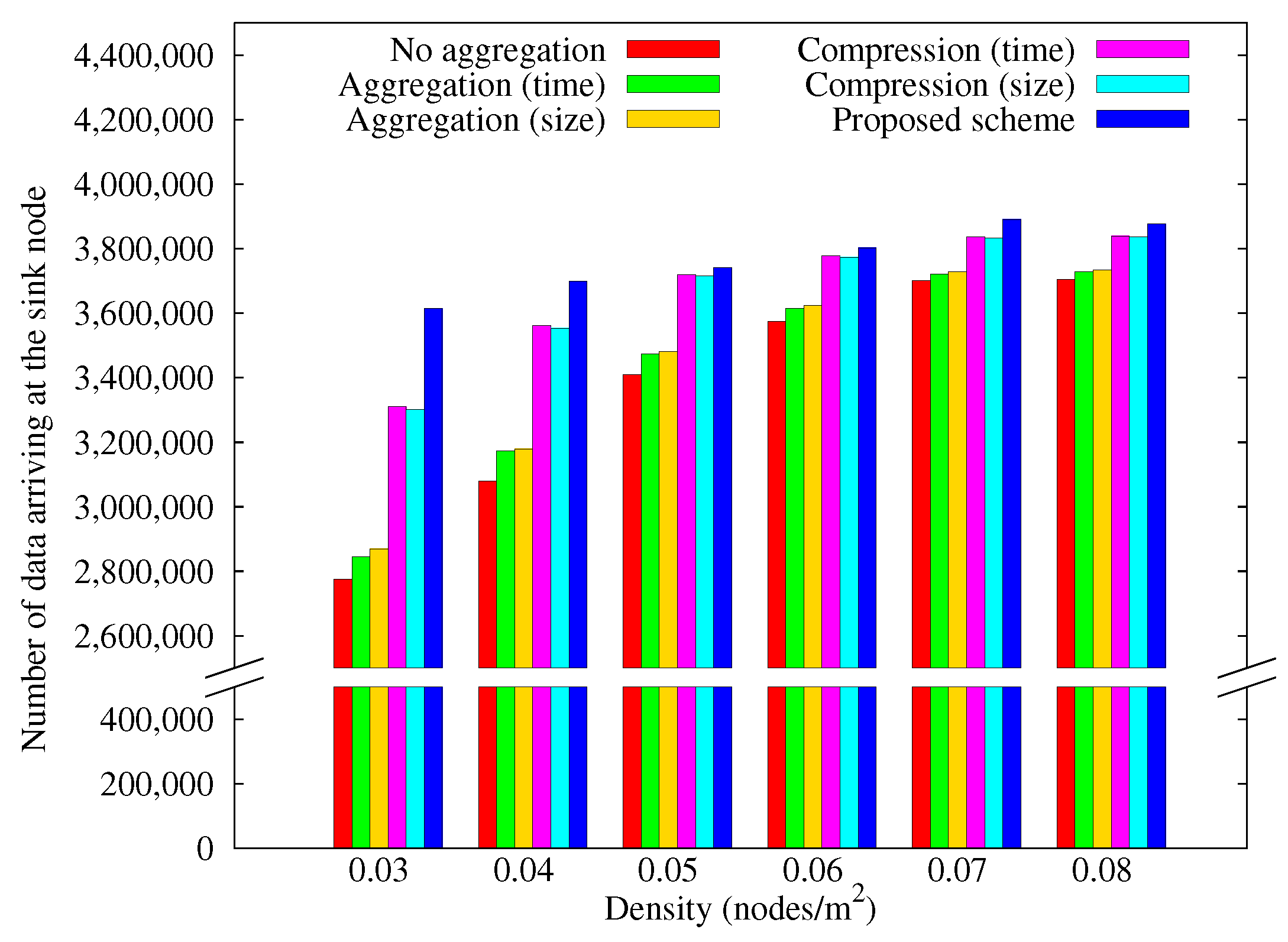
4.2.2. Amount of Data Arriving at the Sink Node
5. Conclusions
Acknowledgments
Author Contributions
Conflicts of Interest
References
- Yick, J.; Mukherjee, B.; Ghosal, D. Wireless sensor network survey. Comput. Netw. 2008, 52, 2292–2330. [Google Scholar] [CrossRef]
- Akyildiz, I.F.; Su, W.; Sankarasubramaniam, Y.; Cayirci, E. Wireless sensor networks: A survey. Comput. Netw. 2002, 38, 393–422. [Google Scholar] [CrossRef]
- Sudevalayam, S.; Kulkarni, P. Energy harvesting sensor nodes: Survey and implications. IEEE Commun. Surv. Tutor. 2011, 13, 443–461. [Google Scholar] [CrossRef]
- Raghunathan, V.; Schurgers, C.; Park, S.; Srivastava, M.B. Energy-aware wireless microsensor networks. IEEE Signal Process. Mag. 2002, 19, 40–50. [Google Scholar] [CrossRef]
- Raghunathan, V.; Kansal, A.; Hsu, J.; Friedman, J.; Srivastava, M. Design considerations for solar energy harvesting wireless embedded systems. In Proceedings of the 4th International Symposium on Information Processing in Sensor Networks, Los Angeles, CA, USA, 15 April 2005; p. 64. [Google Scholar]
- Minami, M.; Morito, T.; Morikawa, H.; Aoyama, T. Solar biscuit: A battery-less wireless sensor network system for environmental monitoring applications. In Proceedings of the 2nd International Workshop on Networked Sensing Systems, San Diego, CA, USA, 1 June 2005. [Google Scholar]
- Meninger, S.; Mur-Miranda, J.O.; Amirtharajah, R.; Chandrakasan, A.P.; Lang, J.H. Vibration-to-electric energy conversion. IEEE Trans. VLSI Syst. 2001, 9, 64–76. [Google Scholar] [CrossRef]
- Ottman, G.K.; Hofmann, H.F.; Bhatt, A.C.; Lesieutre, G.A. Adaptive piezoelectric energy harvesting circuit for wireless remote power supply. IEEE Trans. Power Electron. 2002, 17, 669–676. [Google Scholar] [CrossRef]
- Li, S.; Yuan, J.; Lipson, H. Ambient wind energy harvesting using cross-flow fluttering. J. Appl. Phys. 2011, 109. [Google Scholar] [CrossRef]
- Weimer, M.A.; Paing, T.S.; Zane, R.A. Remote area wind energy harvesting for low-power autonomous sensors. System 2006, 2, 2. [Google Scholar]
- Stordeur, M.; Stark, I. Low power thermoelectric generator-self-sufficient energy supply for micro systems. In Proceedings of the XVI International Conference on Thermoelectrics, Dresden, Germany, 26–29 August 2002; pp. 575–577. [Google Scholar]
- Roundy, S.J. Energy Scavenging for Wireless Sensor Nodes with a Focus on Vibration to Electricity Conversion. Ph.D. Thesis, University of California, Berkeley, CA, USA, 2003. [Google Scholar]
- Yoo, H.; Shim, M.; Kim, D. Dynamic duty-cycle scheduling schemes for energy-harvesting wireless sensor networks. IEEE Commun. Lett. 2012, 16, 202–204. [Google Scholar] [CrossRef]
- Vullers, R.J.; van Schaijk, R.; Visser, H.J.; Penders, J.; van Hoof, C. Energy harvesting for autonomous wireless sensor networks. IEEE Solid-State Circuits Mag. 2010, 2, 29–38. [Google Scholar] [CrossRef]
- Basagni, S.; Naderi, M.Y.; Petrioli, C.; Spenza, D. Wireless sensor networks with energy harvesting. In Mobile Ad Hoc Networking: The Cutting Edge Directions; Wiley: New York, NY, USA, 2013; pp. 701–736. [Google Scholar]
- Fasolo, E.; Rossi, M.; Widmer, J.; Zorzi, M. In-network aggregation techniques for wireless sensor networks: A survey. IEEE Wirel. Commun. 2007, 14, 70–87. [Google Scholar] [CrossRef]
- Rajagopalan, R.; Varshney, P.K. Data aggregation techniques in sensor networks: A survey. IEEE Commun. Surv. Tutor. 2006, 8, 48–63. [Google Scholar] [CrossRef]
- Fall, K. A delay-tolerant network architecture for challenged internets. In Proceedings of the 2003 Conference on Applications, Technologies, Architectures, and Protocols for Computer Communications, Karlsruhe, Germany, 25–29 Auguest 2003; ACM: New York, NY, USA, 2003; pp. 27–34. [Google Scholar]
- Krishnamachari, L.; Estrin, D.; Wicker, S. The impact of data aggregation in wireless sensor networks. In Proceedings of the 22nd International Conference on Distributed Computing Systems Workshops, Vienna, Austria, 2–5 July 2002; pp. 575–578. [Google Scholar]
- Heinzelman, W.B. Application-Specific Protocol Architectures for Wireless Networks. Ph.D. Thesis, Massachusetts Institute of Technology, Cambridge, MA, USA, June 2000. [Google Scholar]
- Voigt, T.; Dunkels, A.; Alonso, J. Solar-aware Clustering In Wireless Sensor Networks. In Proceedings of the Ninth International Symposium on Computers And Communications, Alexandria, Egypt, 28–1 July 2004; pp. 238–243. [Google Scholar]
- Chatterjea, S.; Havinga, P. A dynamic data aggregation scheme for wireless sensor networks. In Proceedings of the 14th Workshop on Circuits, Systems and Signal Processing, Veldhoven, the Netherlands, 26–27 November 2003. [Google Scholar]
- Intanagonwiwat, C.; Govindan, R.; Estrin, D.; Heidemann, J.; Silva, F. Directed diffusion for wireless sensor networking. IEEE/ACM Trans. Netw. 2003, 11, 2–16. [Google Scholar] [CrossRef]
- Ghaffariyan, P. An effective data aggregation mechanism for wireless sensor networks. In Proceedings of the 6th International Conference on Wireless Communications Networking and Mobile Computing, Chengdu, China, 23–25 September 2010; pp. 1–4. [Google Scholar]
- Boyd, S.; Ghosh, A.; Prabhakar, B.; Shah, D. Gossip algorithms: Design, analysis and applications. In Proceedings of the 24th Annual Joint Conference of the IEEE Computer and Communications Societies, Miami, FL, USA, 13–17 March 2005; Volume 3, pp. 1653–1664. [Google Scholar]
- Kimura, N.; Latifi, S. A survey on data compression in wireless sensor networks. In Proceedings of the International Conference on Information Technology: Coding and Computing, Las Vegas, NV, USA, 4–6 April 2005; Volume 2, pp. 8–13. [Google Scholar]
- Srisooksai, T.; Keamarungsi, K.; Lamsrichan, P.; Araki, K. Practical data compression in wireless sensor networks: A survey. J. Netw. Comput. Appl. 2012, 35, 37–59. [Google Scholar] [CrossRef]
- Sadler, C.M.; Martonosi, M. Data compression algorithms for energy-constrained devices in delay tolerant networks. In Proceedings of the 4th International Conference on Embedded Networked Sensor Systems, Boulder, CO, USA, 31 October–3 November 2006; pp. 265–278. [Google Scholar]
- Petrovic, D.; Shah, R.C.; Ramchandran, K.; Rabaey, J. Data funneling: Routing with aggregation and compression for wireless sensor networks. In Proceedings of the First IEEE International Workshop on Sensor Network Protocols and Applications, Anchorage, AK, USA, 11 May 2003; pp. 156–162. [Google Scholar]
- Arici, T.; Gedik, B.; Altunbasak, Y.; Liu, L. PINCO: A pipelined in-network compression scheme for data collection in wireless sensor networks. In Proceedings of the 12th International Conference on Computer Communications and Networks, Dallas, TX, USA, 22 October 2003; pp. 539–544. [Google Scholar]
- Kasirajan, P.; Larsen, C.; Jagannathan, S. A new data aggregation scheme via adaptive compression for wireless sensor networks. ACM Trans. Sensor Netw. 2012, 9, 5. [Google Scholar] [CrossRef]
- Zanella, A.; Bazzi, A.; Pasolini, G.; Masini, B.M. On the Impact of Routing Strategies on the Interference of Ad Hoc Wireless Networks. IEEE Trans. Commun. 2013, 61, 4322–4333. [Google Scholar] [CrossRef]
- Zanella, A.; Bazzi, A.; Masini, B.M. Relay Selection Analysis for an Opportunistic Two-Hop Multi-User System in a Poisson Field of Nodes. IEEE Trans. Wirel. Commun. 2017, 16, 1281–1293. [Google Scholar] [CrossRef]
- Zanella, A.; Masini, B.M. Connectivity analysis in power controlled decentralized wireless networks. In Proceedings of the 7th International Symposium on Wireless Communication Systems, York, UK, 19–22 September 2010; pp. 877–881. [Google Scholar]
- La Palombara, C.; Tralli, V.; Masini, B.M.; Conti, A. Relay-assisted diversity communications. IEEE Trans. Veh. Technol. 2013, 62, 415–421. [Google Scholar] [CrossRef]
- Roundy, S.; Steingart, D.; Frechette, L.; Wright, P.; Rabaey, J. Power sources for wireless sensor networks. In Wireless Sensor Networks; Springer: Berlin/Heidelberg, Germany, 2004; pp. 1–17. [Google Scholar]
- Kansal, A.; Potter, D.; Srivastava, M.B. Performance aware tasking for environmentally powered sensor networks. ACM SIGMETRICS Perform. Eval. Rev. 2004, 32, 223–234. [Google Scholar] [CrossRef]
- Yang, Y.; Wang, L.; Noh, D.K.; Le, H.K.; Abdelzaher, T.F. Solarstore: Enhancing data reliability in solar-powered storage-centric sensor networks. In Proceedings of the 7th International Conference on Mobile Systems, Applications, and Services, Wroclaw, Poland, 22–25 June 2009; pp. 333–346. [Google Scholar]
- Cammarano, A.; Petrioli, C.; Spenza, D. Pro-energy: A novel energy prediction model for solar and wind energy-harvesting wireless sensor networks. In Proceedings of the 9th International Conference on Mobile Adhoc and Sensor Systems, Las Vegas, NV, USA, 8–11 October 2012; pp. 75–83. [Google Scholar]
- Noh, D.; Kim, J.; Lee, J.; Lee, D.; Kwon, H.; Shin, H. Priority-based routing for solar-powered wireless sensor networks. In Proceedings of the 2nd International Symposium on the Wireless Pervasive Computing, San Juan, PR, USA, 5–7 February 2007. [Google Scholar]
- Kang, M.J.; Jeong, S.; Yoon, I.; Noh, D.K. Energy-aware determination of compression for low latency in solar-powered wireless sensor networks. Int. J. Distrib. Sens. Netw. 2017, 13. [Google Scholar] [CrossRef]
- Stojmenovic, I. Handbook of Sensor Networks: Algorithms and Architectures; John Wiley & Sons: New York, NY, USA, 2005; Volume 49. [Google Scholar]
- Melodia, T.; Pompili, D.; Akyildiz, I.F. Optimal local topology knowledge for energy efficient geographical routing in sensor networks. In Proceedings of the 23rd Annual Joint Conference of the IEEE Computer and Communications Societies, Hong Kong, China, 7–11 March 2004; Volume 3, pp. 1705–1716. [Google Scholar]
- Kansal, A.; Hsu, J.; Zahedi, S.; Srivastava, M.B. Power management in energy harvesting sensor networks. ACM Trans. Embed. Comput. Syst. 2007, 6, 32. [Google Scholar] [CrossRef]
- Piorno, J.R.; Bergonzini, C.; Atienza, D.; Rosing, T.S. Prediction and management in energy harvested wireless sensor nodes. In Proceedings of the 1st International Conference on Wireless Communication, Vehicular Technology, Information Theory and Aerospace & Electronic Systems Technology, Aalborg, Denmark, 17–20 May 2009; pp. 6–10. [Google Scholar]
- Moser, C.; Thiele, L.; Brunelli, D.; Benini, L. Adaptive power management in energy harvesting systems. In Proceedings of the Conference on Design, Automation and Test in Europe, Nice, France, 16–20 April 2007; pp. 773–778. [Google Scholar]
- Yi, J.M.; Kang, M.J.; Noh, D.K. SolarCastalia: Solar energy harvesting wireless sensor network simulator. Int. J. Distrib. Sens. Netw. 2015, 11. [Google Scholar] [CrossRef]
- Karp, B.; Kung, H.T. GPSR: Greedy perimeter stateless routing for wireless networks. In Proceedings of the 6th Annual International Conference on Mobile Computing and Networking, Boston, MA, USA, 6–11 August 2000; pp. 243–254. [Google Scholar]


| Harvesting Technology | Power Density |
|---|---|
| Solar cells (outdoors at noon) | 15 |
| Piezoelectric (shoe inserts) | 330 |
| Vibration (small microwave oven) | 116 |
| Thermoelectric (10 ℃ gradient) | 40 |
| Acoustic noise (100 dB) | 960 |
| Parameters | Values |
|---|---|
| Number of nodes | 100 |
| Node topology | Random |
| Routing algorithm | Minimum depth tree (MDT) |
| Transmission range | 10∼20 m |
| 1 h | |
| 300 s | |
| 60 s | |
| 102 bytes | |
| 1024 bytes | |
| 8∼80 bytes |
© 2017 by the authors. Licensee MDPI, Basel, Switzerland. This article is an open access article distributed under the terms and conditions of the Creative Commons Attribution (CC BY) license (http://creativecommons.org/licenses/by/4.0/).
Share and Cite
Yoon, I.; Kim, H.; Noh, D.K. Adaptive Data Aggregation and Compression to Improve Energy Utilization in Solar-Powered Wireless Sensor Networks. Sensors 2017, 17, 1226. https://doi.org/10.3390/s17061226
Yoon I, Kim H, Noh DK. Adaptive Data Aggregation and Compression to Improve Energy Utilization in Solar-Powered Wireless Sensor Networks. Sensors. 2017; 17(6):1226. https://doi.org/10.3390/s17061226
Chicago/Turabian StyleYoon, Ikjune, Hyeok Kim, and Dong Kun Noh. 2017. "Adaptive Data Aggregation and Compression to Improve Energy Utilization in Solar-Powered Wireless Sensor Networks" Sensors 17, no. 6: 1226. https://doi.org/10.3390/s17061226
APA StyleYoon, I., Kim, H., & Noh, D. K. (2017). Adaptive Data Aggregation and Compression to Improve Energy Utilization in Solar-Powered Wireless Sensor Networks. Sensors, 17(6), 1226. https://doi.org/10.3390/s17061226