Analysis of Maneuvering Targets with Complex Motions by Two-Dimensional Product Modified Lv’s Distribution for Quadratic Frequency Modulation Signals

Abstract
:1. Introduction
2. 2D-PMLVD with QFM Signal
2.1. 2D-PMLVD with Mono-QFM Signal
2.2. 2D-PMLVD with Multi-QFM Signals
- , , and .
- , , and .
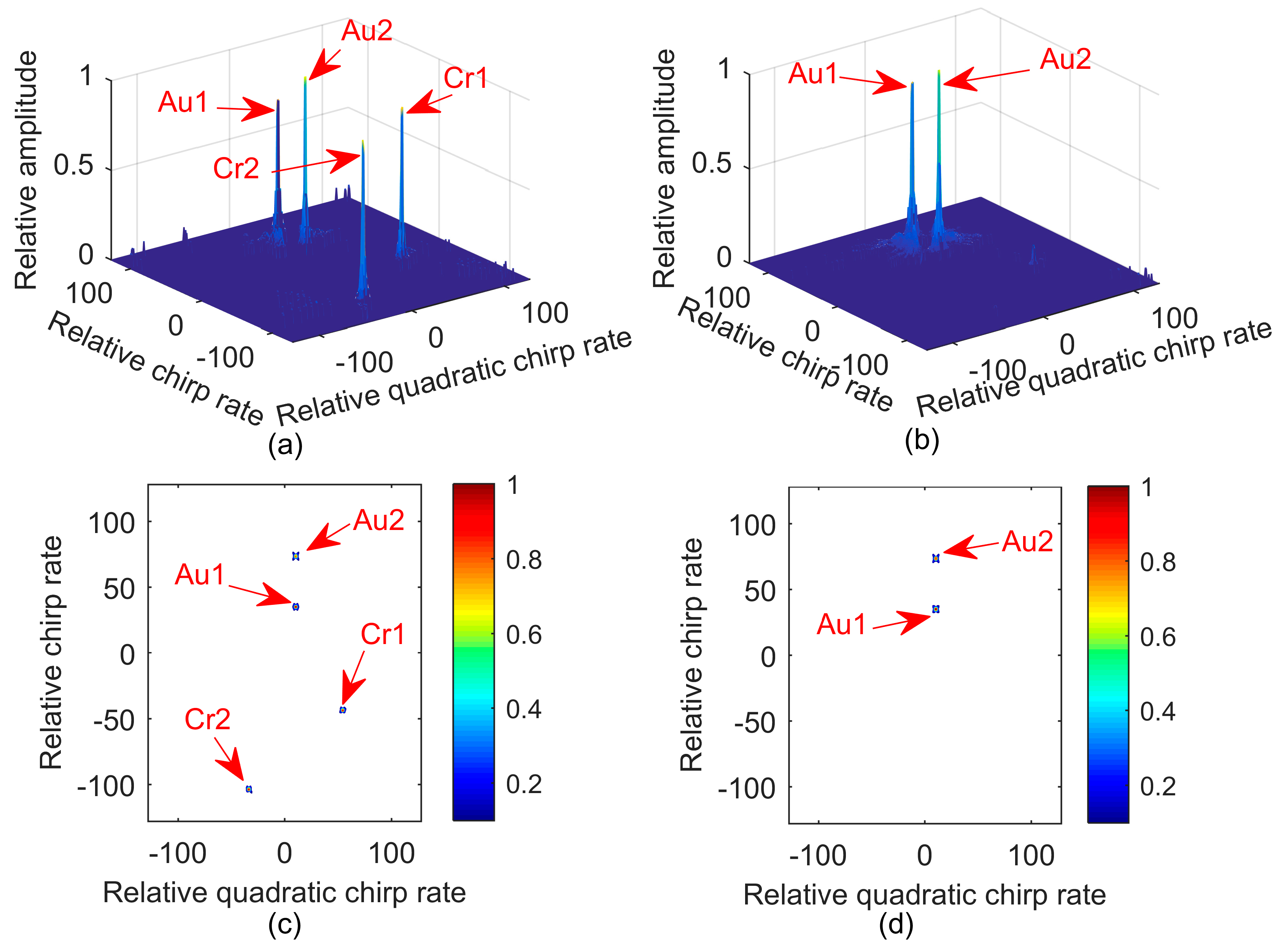
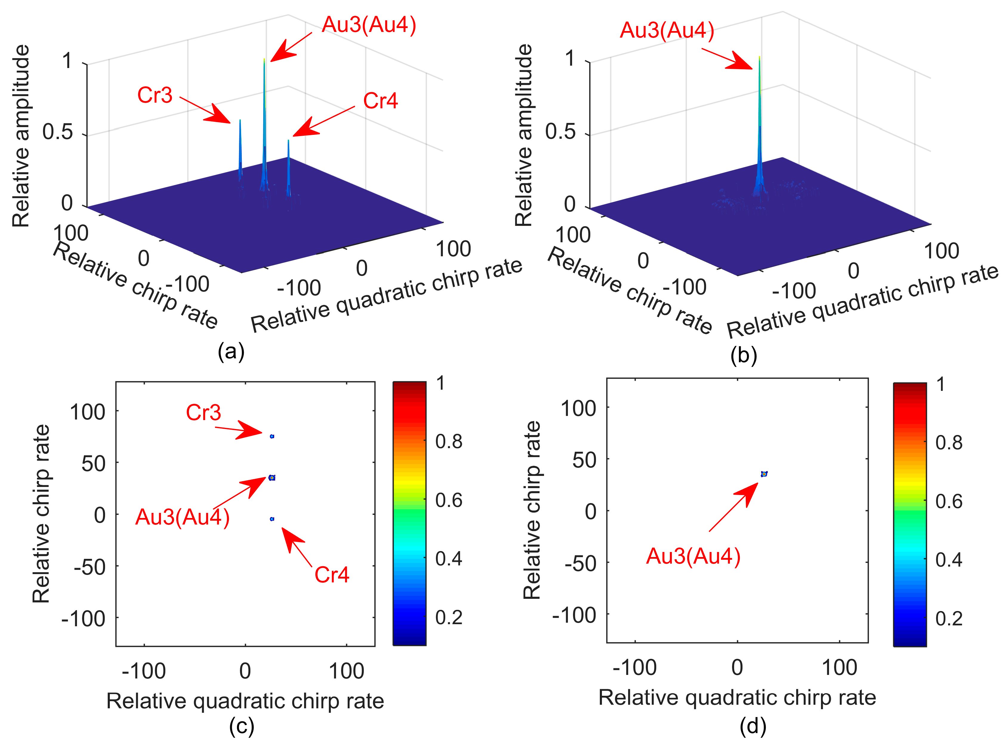
2.2.1. Case One
2.2.2. Case Two
2.3. Parameter Selection and Resolution
2.3.1. Selection of and
2.3.2. Selection of
2.3.3. Resolution
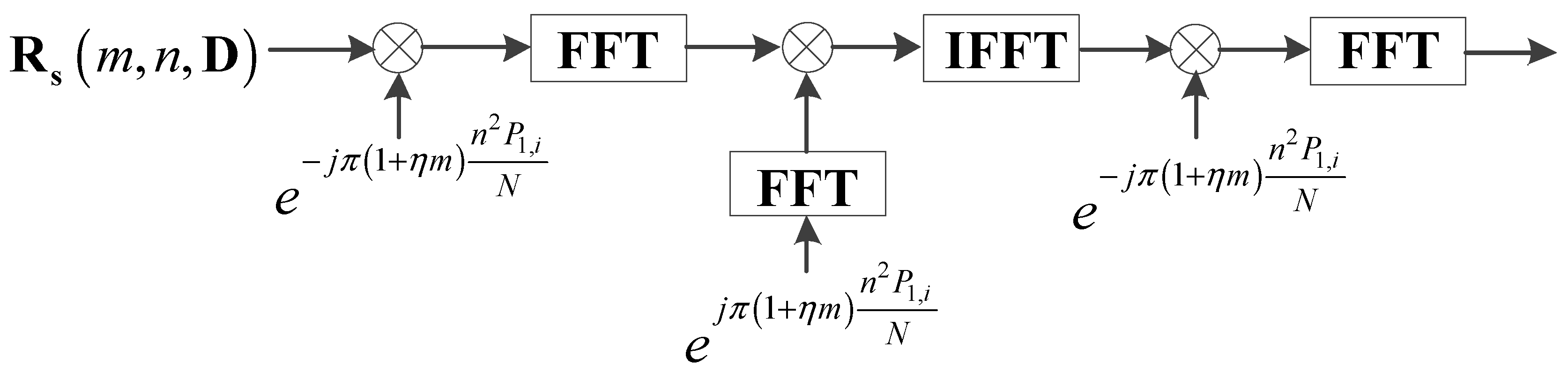
3. Implementation
4. Analyses of Anti-Noise Performance and Computational Cost
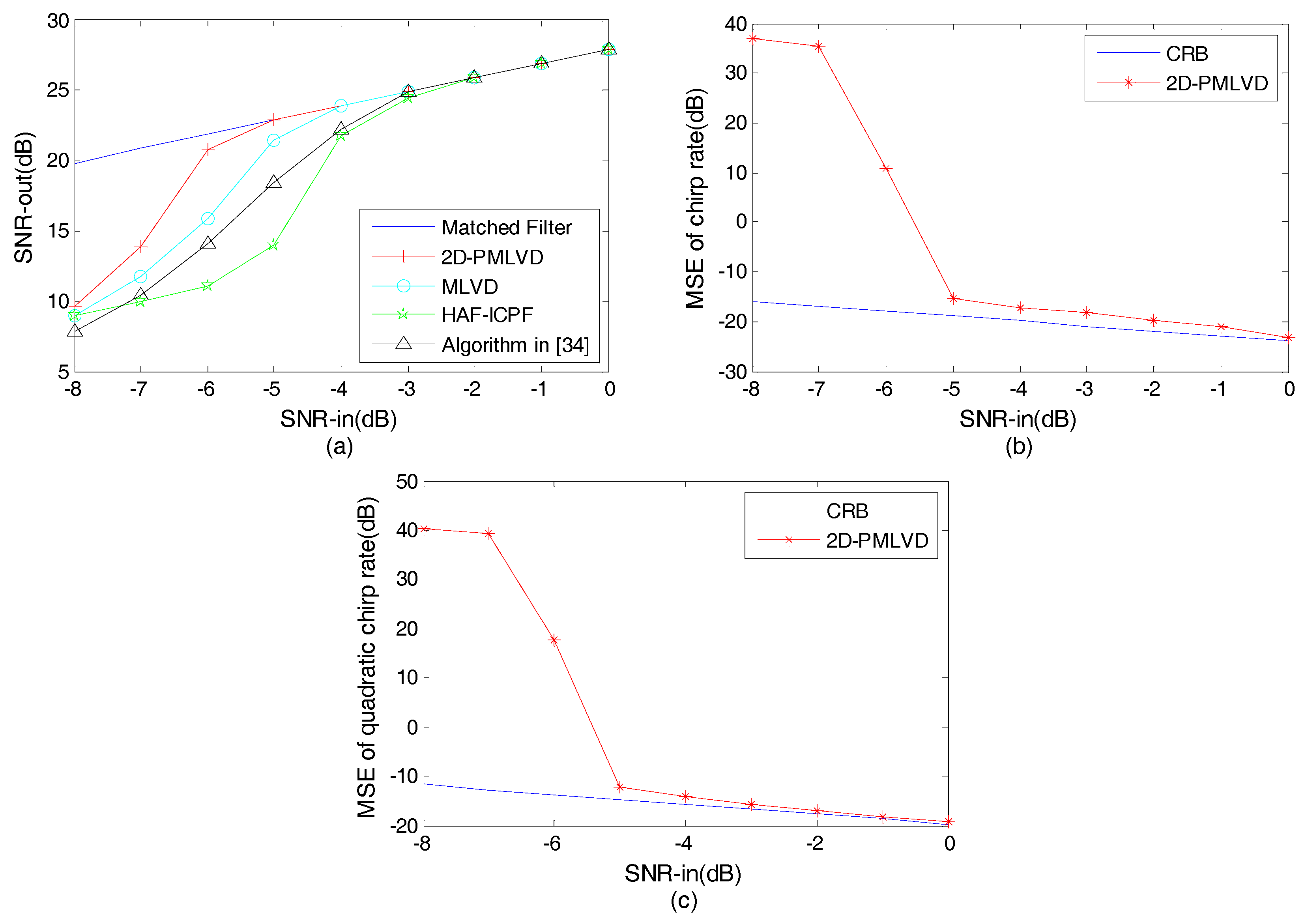
4.1. Anti-Noise Performance Analysis
4.2. Computational Cost
5. Conclusions
Acknowledgments
Author Contributions
Conflicts of Interest
References
- Zhou, C.; Gu, Y.; He, S.; Shi, Z. A robust and efficient algorithm for coprime array adaptive beamforming. IEEE Trans. Veh. Technol. 2017, PP. [Google Scholar] [CrossRef]
- Barbarossa, S.; Petrone, V. Analysis of polynomial-phase signals by the integrated generalized ambiguity function. IEEE Trans. Signal Process. 1997, 45, 316–327. [Google Scholar] [CrossRef]
- Gu, Y.; Leshem, A. Robust adaptive beamforming based on interference covariance matrix reconstruction and steering vector estimation. IEEE Trans. Signal Process. 2012, 60, 3881–3885. [Google Scholar]
- Song, Y.E.; Wang, C.G.; Shi, P. Algorithm based on the linear canonical transform for qfm signal parameters estimation. IET Signal Process. 2016, 10, 318–324. [Google Scholar] [CrossRef]
- Gu, Y.; Goodman, N.A. Information-theoretic compressive sensing kernel optimization and bayesian Cramér-Rao bound for time delay estimation. IEEE Trans. Signal Process. 2017, PP. [Google Scholar] [CrossRef]
- Shi, Z.; Zhou, C.; Gu, Y.; Goodman, N.A.; Qu, F. Source estimation using coprime array: A sparse reconstruction perspective. IEEE Sens. J. 2017, 17, 755–765. [Google Scholar] [CrossRef]
- Wang, P.; Li, H.; Djurovic, I.; Himed, B. Performance of instantaneous frequency rate estimation using high-order phase function. IEEE Trans. Signal Process. 2010, 58, 2415–2421. [Google Scholar] [CrossRef]
- Mo, S.; Wang, Y.; Liu, C. An estimation algorithm for phase errors in synthetic aperture radar imagery. IEEE Geosci. Remote Sens. Lett. 2015, 12, 1818–1822. [Google Scholar]
- Wang, B.; Zhang, Y.D.; Wang, W. Robust doa estimation in the presence of mis-calibrated sensors. IEEE Signal Process. Lett. 2017, PP. [Google Scholar] [CrossRef]
- Guo, M.; Tao, C.; Wang, B. An improved doa estimation approach using coarray interpolation and matrix denoising. Sensors 2017, 17, 1140. [Google Scholar] [CrossRef] [PubMed]
- Zhou, Y.; Zhang, Y.D.; Shi, Z.; Jin, T.; Wu, X. Compressive Sensing Based Coprime Array Direction-of-Arrival Estimation. IET Commun. 2017, in press. [Google Scholar] [CrossRef]
- Berizzi, F.; Mese, E.D.; Diani, M.; Martorella, M. High-resolution isar imaging of maneuvering targets by means of the range instantaneous doppler technique: Modeling and performance analysis. IEEE Trans. Image Process. 2001, 10, 1880–1890. [Google Scholar] [CrossRef] [PubMed]
- Li, Y.; Xing, M.; Su, J.; Quan, Y. A new algorithm of isar imaging for maneuvering targets with low snr. IEEE Trans. Aerosp. Electron. Syst. 2013, 49, 543–557. [Google Scholar] [CrossRef]
- Zhu, D.; Li, Y.; Zhu, Z. A keystone transform without interpolation for sar ground moving-target imaging. IEEE Geosci. Remote Sens. Lett. 2007, 4, 18–22. [Google Scholar] [CrossRef]
- Xing, M.; Wu, R.; Bao, Z. High resolutio isar imaging of high speed moving targets. IEE Proc. Radar Sonar Navig. 2005, 152, 58–67. [Google Scholar] [CrossRef]
- Wahl, D.E.; Eichel, P.H.; Ghiglia, D.C.; Jakowatz, C.V., Jr. Phase gradient autofocus—A robust tool for high resolution sar phase correction. IEEE Trans. Aerosp. Electron. Syst. 1994, 30, 827–835. [Google Scholar] [CrossRef]
- Xi, L.; Liu, G.; Ni, J. Autofocusing of isar images based on entropy minimization. IEEE Trans. Aerosp. Electron. Syst. 1999, 35, 1240–1252. [Google Scholar] [CrossRef]
- Almeida, L.B. The fractional fourier transform and time-frequency representations. IEEE Trans. Signal Process. 1994, 42, 3084–3091. [Google Scholar] [CrossRef]
- Lv, X.; Xing, M.; Wan, C.; Zhang, S. Isar imaging of maneuvering targets based on the range centroid doppler technique. IEEE Trans. Image Process. 2010, 19, 141–153. [Google Scholar] [PubMed]
- Bi, G.; Li, X.; Samson See, C.M. Lfm signal detection using lpp-hough transform. Signal Process. 2011, 91, 1432–1443. [Google Scholar] [CrossRef]
- Lv, X.; Bi, G.; Wan, C.; Xing, M. Lv’s distribution: Principle, implementation, properties, and performance. IEEE Trans. Signal Process. 2011, 59, 3576–3591. [Google Scholar] [CrossRef]
- Abatzoglou, T.J. Fast maximum likelihood joint estimation of frequency and frequency rate. In Proceedings of the IEEE International Conference on Acoustics, Speech, and Signal Processing, ICASSP ’86, Tokyo, Japan, 7–11 April 1986; pp. 1409–1412. [Google Scholar]
- Zheng, J. Fast parameter estimation algorithm for cubic phase signal based on quantifying effects of doppler frequency shift. Prog. Electromagn. Res. 2013, 142, 57–74. [Google Scholar] [CrossRef]
- Wu, L.; Wei, X.; Yang, D.; Wang, H. Isar imaging of targets with complex motion based on discrete chirp fourier transform for cubic chirps. IEEE Trans. Geosci. Remote Sens. 2012, 50, 4201–4212. [Google Scholar] [CrossRef]
- Barbarossa, S.; Scaglione, A.; Giannakis, G.B. Product high-order ambiguity function for multicomponent polynomial-phase signal modeling. IEEE Trans. Signal Process. 1998, 46, 691–708. [Google Scholar] [CrossRef]
- O’Shea, P. A new technique for instantaneous frequency rate estimation. IEEE Signal Process. Lett. 2002, 9, 251–252. [Google Scholar] [CrossRef]
- O’Shea, P. A fast algorithm for estimating the parameters of a quadratic fm signal. IEEE Trans. Signal Process. 2004, 52, 385–393. [Google Scholar] [CrossRef]
- Wang, Y.; Jiang, Y. Inverse synthetic aperture radar imaging of maneuvering target based on the product generalized cubic phase function. IEEE Geosci. Remote Sens. Lett. 2011, 8, 958–962. [Google Scholar] [CrossRef]
- Wang, Y.; Jiang, Y. Isar imaging of a ship target using product high-order matched-phase transform. IEEE Geosci. Remote Sens. Lett. 2009, 6, 658–661. [Google Scholar] [CrossRef]
- Wang, Y. Inverse synthetic aperture radar imaging of manoeuvring target based on range-instantaneous- doppler and range-instantaneous-chirp-rate algorithms. IET Radar Sonar Navig. 2012, 6, 921–928. [Google Scholar] [CrossRef]
- Bai, X.; Tao, R.; Wang, Z.; Wang, Y. Isar imaging of a ship target based on parameter estimation of multicomponent quadratic frequency-modulated signals. IEEE Trans. Geosci. Remote Sens. 2014, 52, 1418–1429. [Google Scholar] [CrossRef]
- Zheng, J.; Su, T.; Zhang, L.; Zhu, W. Isar imaging of targets with complex motion based on the chirp rate—Quadratic chirp rate distribution. IEEE Trans. Geosci. Remote Sens. 2014, 52, 7276–7289. [Google Scholar] [CrossRef]
- Li, Y.; Su, T.; Zheng, J.; He, X. ISAR imaging of targets with complex motions based on modified lv’s distribution for cubic phase signal. IEEE J. Sel. Top. Appl. Earth Obs. Remote Sens. 2015, 8, 4775–4784. [Google Scholar] [CrossRef]
- Zheng, J.; Liu, H.; Liao, G.; Su, T. Isar imaging of targets with complex motions based on a noise-resistant parameter estimation algorithm without nonuniform axis. IEEE Sens. J. 2016, 16, 2509–2518. [Google Scholar] [CrossRef]
- Zheng, J.; Su, T.; Zhu, W.; Zhang, L. Isar imaging of nonuniformly rotating target based on a fast parameter estimation algorithm of cubic phase signal. IEEE Trans. Geosci. Remote Sens. 2015, 53, 1–14. [Google Scholar]
- Lv, X.; Xing, M.; Zhang, S.; Bao, Z. Keystone transformation of the wigner-ville distribution for analysis of multicomponent lfm signals. Signal Process. 2009, 89, 791–806. [Google Scholar] [CrossRef]
- Djurovic, I.; Simeunovic, M.; Djukanovic, S.; Wang, P. A hybrid cpf-haf estimation of polynomial-phase signals: Detailed statistical analysis. IEEE Trans. Signal Process. 2012, 60, 5010–5023. [Google Scholar] [CrossRef]
- Claasen, T.A.C.M.; Mecklenbräuker, W.F.G. The wigner distribution—A tool for time-frequency signal analysis—Part II: Discrete time signals. Philips J. Res. 1980, 35, 276–300. [Google Scholar]
- Luo, S.; Bi, G.; Lv, X.; Hu, F. Performance analysis on lv distribution and its applications. Digit. Signal Process. 2013, 23, 797–807. [Google Scholar] [CrossRef]
- Wang, P.; Li, H.; Djurović, I.; Himed, B. Integrated cubic phase function for linear fm signal analysis. IEEE Trans. Aerosp. Electron. Syst. 2010, 46, 963–977. [Google Scholar] [CrossRef]
- Peleg, S.; Porat, B. The cramer-rao lower bound for signals with constant amplitude and polynomial phase. IEEE Trans. Signal Process. 1991, 39, 749–752. [Google Scholar] [CrossRef]
- Peleg, S.; Porat, B. Linear fm signal parameter estimation from discrete-time observations. IEEE Trans. Aerosp. Electron. Syst. 1991, 27, 607–616. [Google Scholar] [CrossRef]


| Estimation Algorithm | Computational Cost |
|---|---|
| HAF-ICPF | |
| The algorithm presented in [34] | |
| MLVD | |
| 2D-PMLVD |
© 2017 by the authors. Licensee MDPI, Basel, Switzerland. This article is an open access article distributed under the terms and conditions of the Creative Commons Attribution (CC BY) license (http://creativecommons.org/licenses/by/4.0/).
Share and Cite
Jing, F.; Jiao, S.; Hou, C.; Si, W.; Wang, Y. Analysis of Maneuvering Targets with Complex Motions by Two-Dimensional Product Modified Lv’s Distribution for Quadratic Frequency Modulation Signals. Sensors 2017, 17, 1460. https://doi.org/10.3390/s17061460
Jing F, Jiao S, Hou C, Si W, Wang Y. Analysis of Maneuvering Targets with Complex Motions by Two-Dimensional Product Modified Lv’s Distribution for Quadratic Frequency Modulation Signals. Sensors. 2017; 17(6):1460. https://doi.org/10.3390/s17061460
Chicago/Turabian StyleJing, Fulong, Shuhong Jiao, Changbo Hou, Weijian Si, and Yu Wang. 2017. "Analysis of Maneuvering Targets with Complex Motions by Two-Dimensional Product Modified Lv’s Distribution for Quadratic Frequency Modulation Signals" Sensors 17, no. 6: 1460. https://doi.org/10.3390/s17061460
APA StyleJing, F., Jiao, S., Hou, C., Si, W., & Wang, Y. (2017). Analysis of Maneuvering Targets with Complex Motions by Two-Dimensional Product Modified Lv’s Distribution for Quadratic Frequency Modulation Signals. Sensors, 17(6), 1460. https://doi.org/10.3390/s17061460