A Sensor Dynamic Measurement Error Prediction Model Based on NAPSO-SVM


Abstract
1. Introduction
2. SVM Algorithm
2.1. SVM
2.2. Kernel Function
3. SVM Parameters Optimization Based on NAPSO
3.1. PSO
3.2. NAPSO
| Algorithm 1: NAPSO |
| Input ω, c1, c2, T |
| Output gbest Initialization: x, pbest, gbest while t < maximum number of iterations and gbest > minimum fitness do for each particle do update the velocity v, position , and fitness f′ find a new position in the neighborhood and calculate its fitness value if1 ( < gbest) then if2 () then accept the new position else if2 accept the new position by the simulated annealing operation end if2 else if1 accept the old position l end if1 update the pbest, gbest and Simulated temperature T end for rank all particles by their fitness value, use the better half to replace the other half. t = t + 1 end while return the gbest |
3.3. Optimization Process
- Step 1:
- Initialize the NAPSO algorithm, set the number of particles velocity, particles positions and the other parameters. Because the search space is 2-dimensional, the position of each particle contains two variables. Set T to be the simulated temperature; the initial T is 5000 °C, and the lower limit of T is 1 °C. Calculate the fitness value of each particle. The fitness evaluation function is defined as follows:where Yi is the actual value, is the predicted value and n is the number of training samples.
- Step 2:
- According to the fitness value of each particle to set the personal best position pbest and global best position gbest.
- Step 3:
- Update the position l and velocity of each particle. Evaluate the fitness value f′. Then, randomly find a new position in the neighborhood of the particle, calculate the new fitness value () of the new position.
- Step 4:
- Calculate the difference between the fitness value f′ and the new fitness value , .
- Step 5:
- When , keep the original position l. When and , according the Equation (12) accept the new position , if and , replace the original position with the new position. Then, update the pbest and gbest.
- Step 6:
- When the updates of each particle has completed, then rank all of the particles according to the each particle’s fitness value, employ the better half particles’ information to replace the other half particles’ information and update the temperature T = T × 0.9.
- Step 7:
- If the number of iterations is equal to the maximum iterations or the gbest is less than or equal to the least fitness, output the two variables of the gbest; otherwise, return to Step 2.
4. Experiments
4.1. Data Description
4.2. Preprocessing
4.3. Valuation Index
4.4. GSO Algorithm
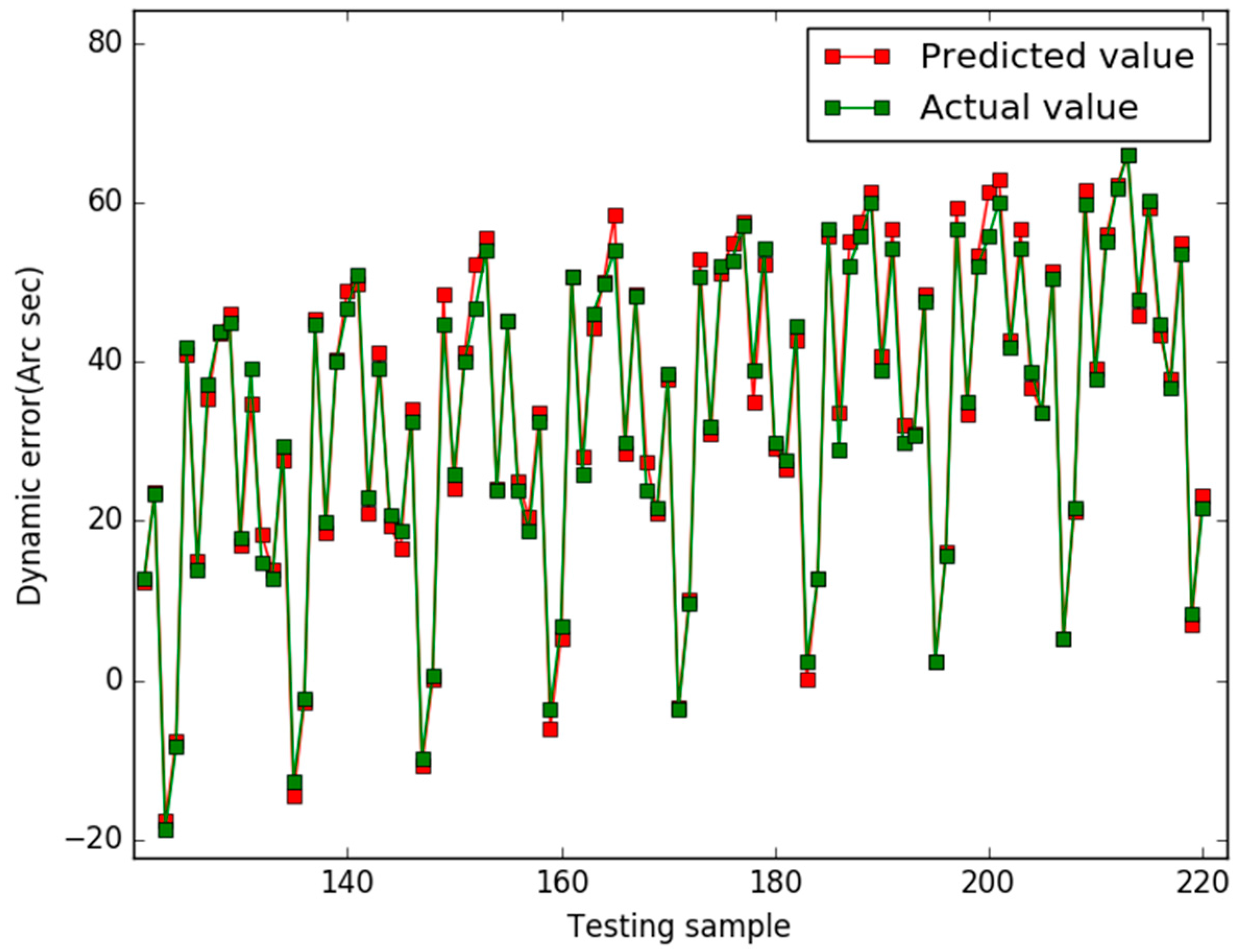
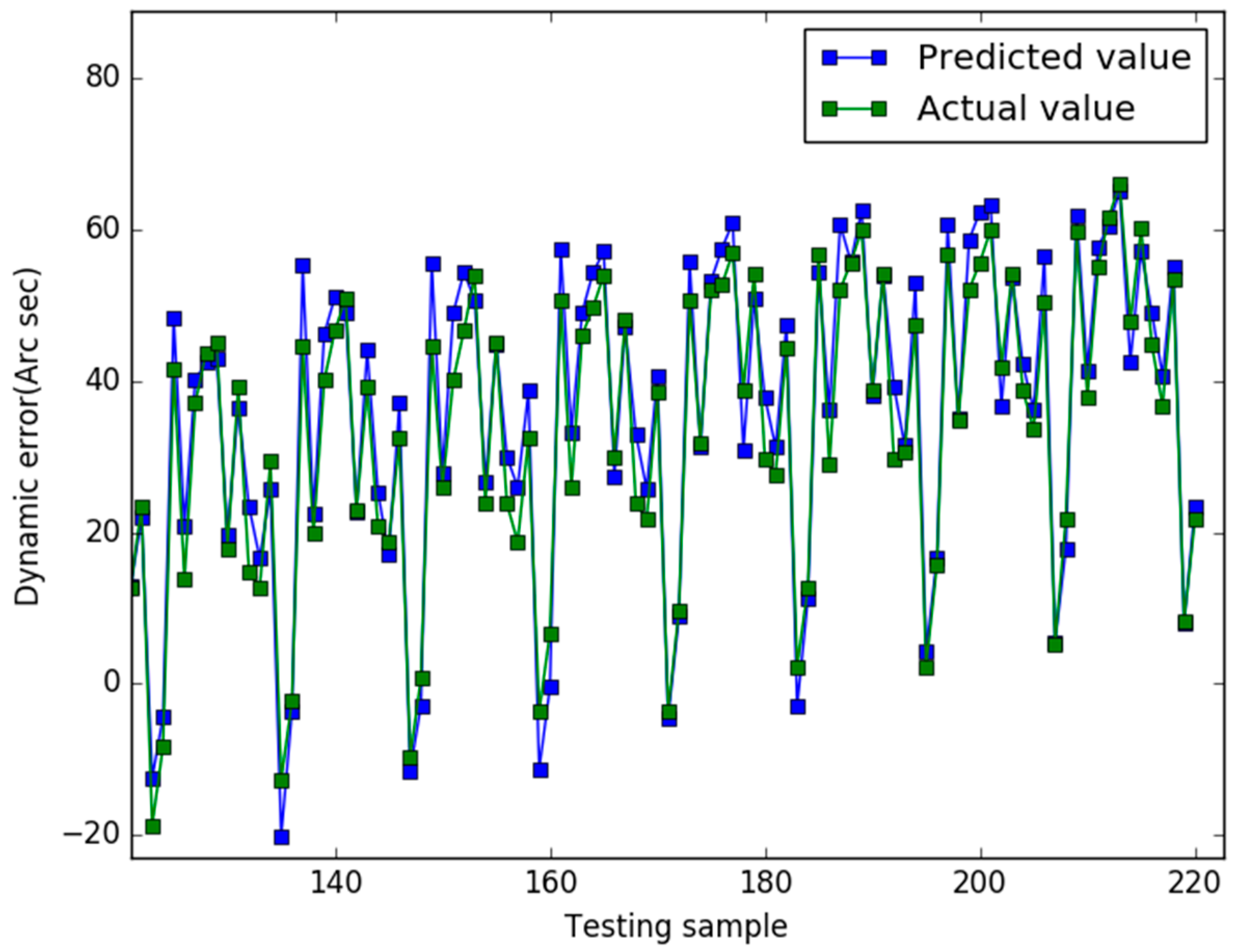
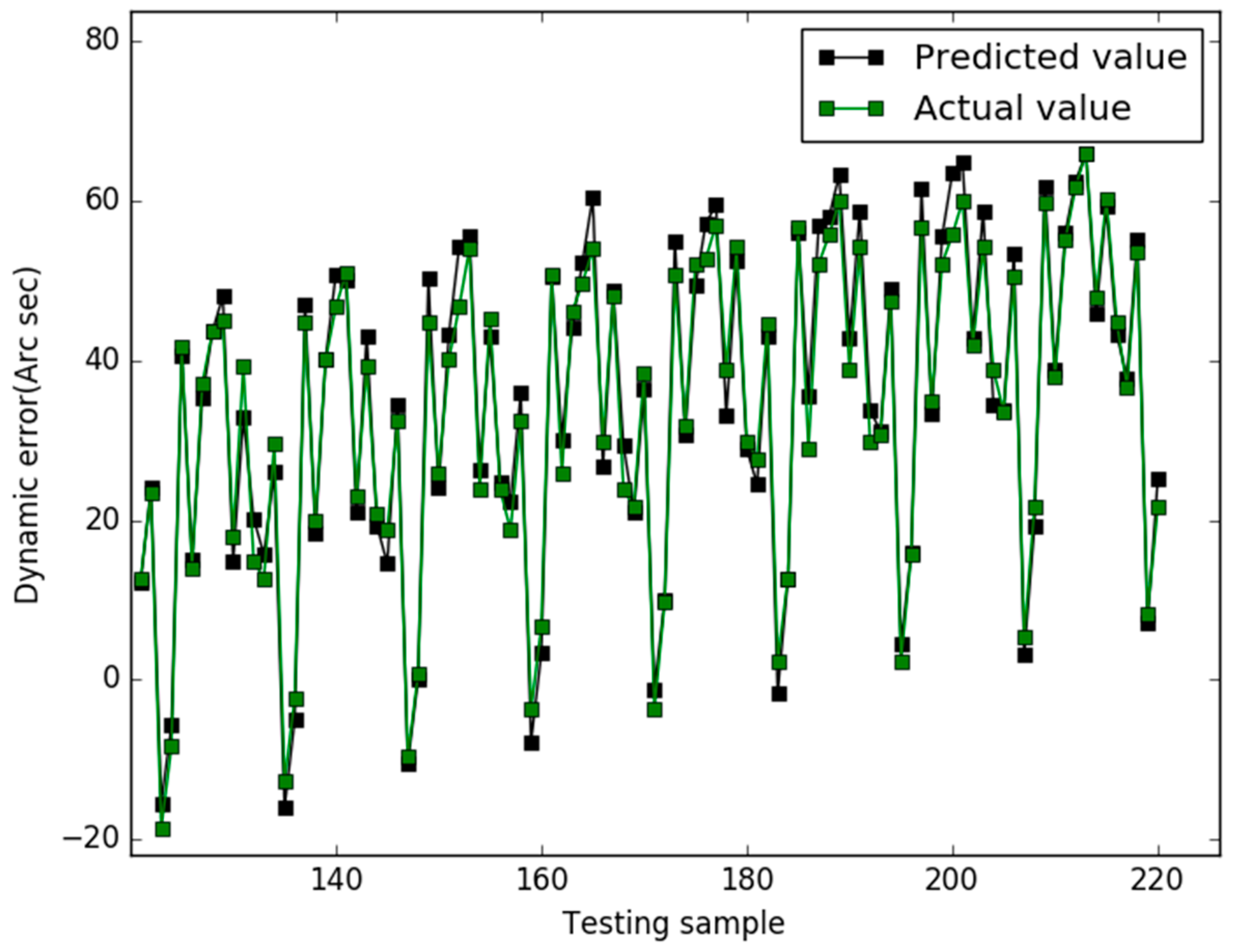
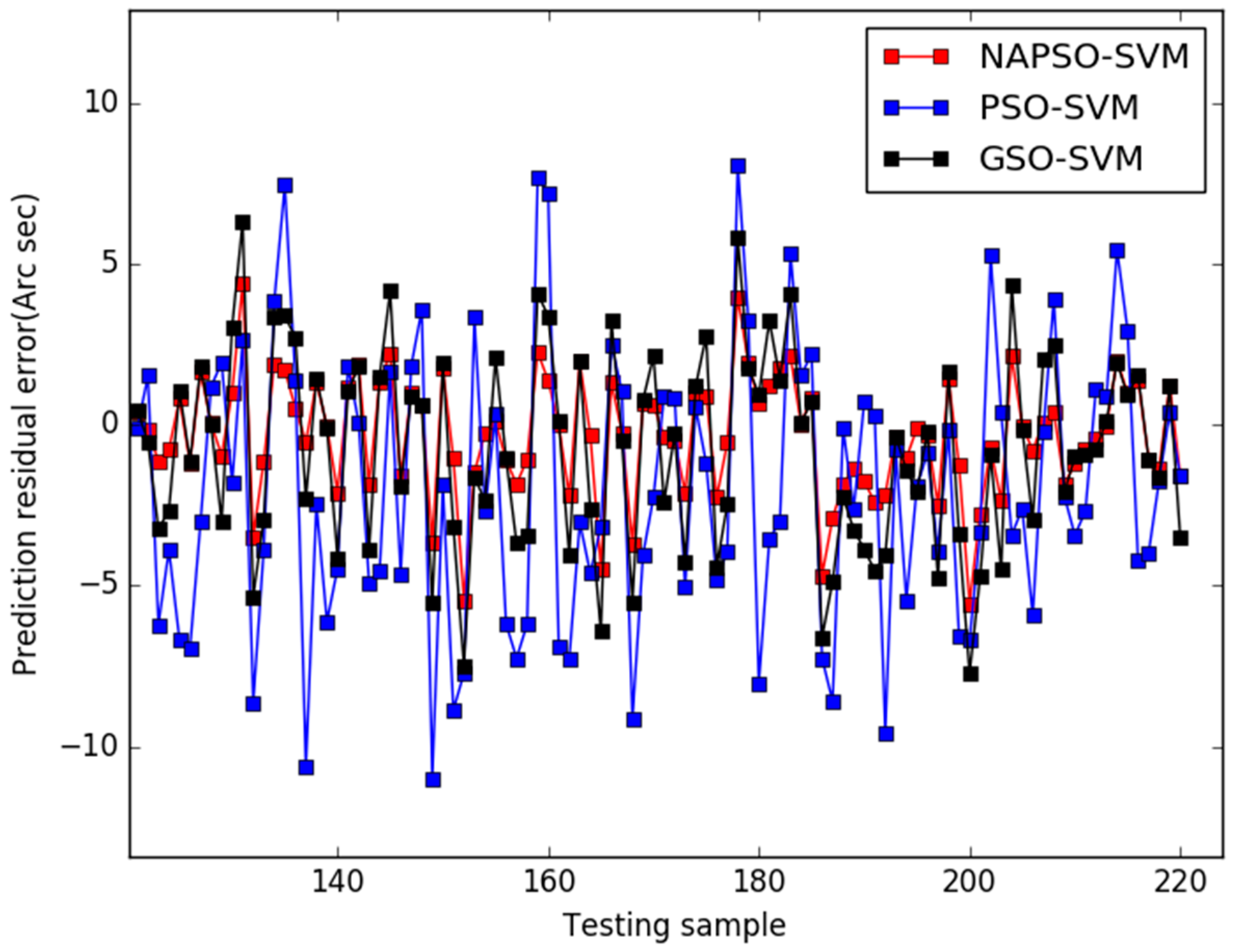
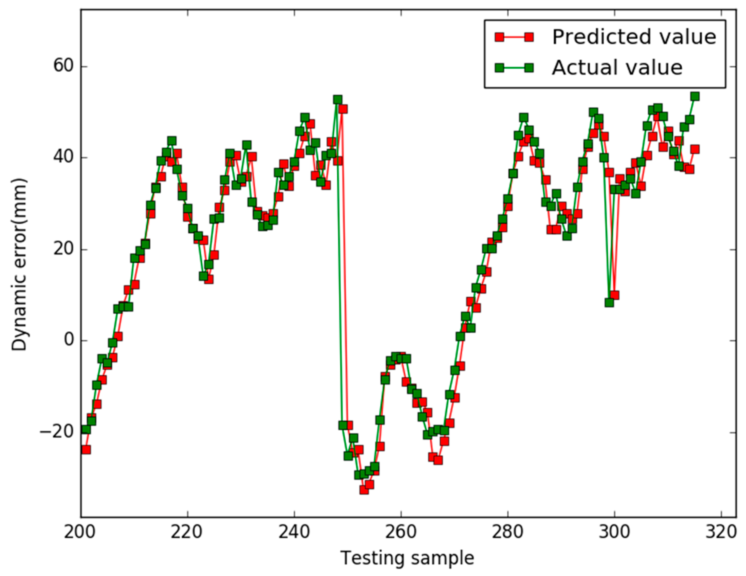
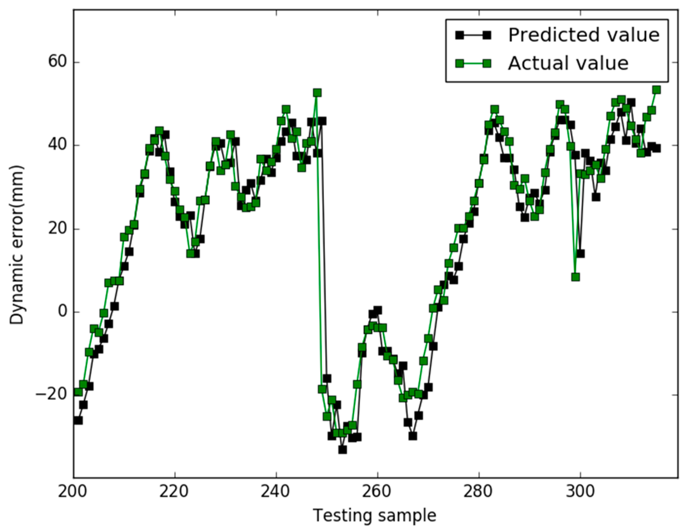
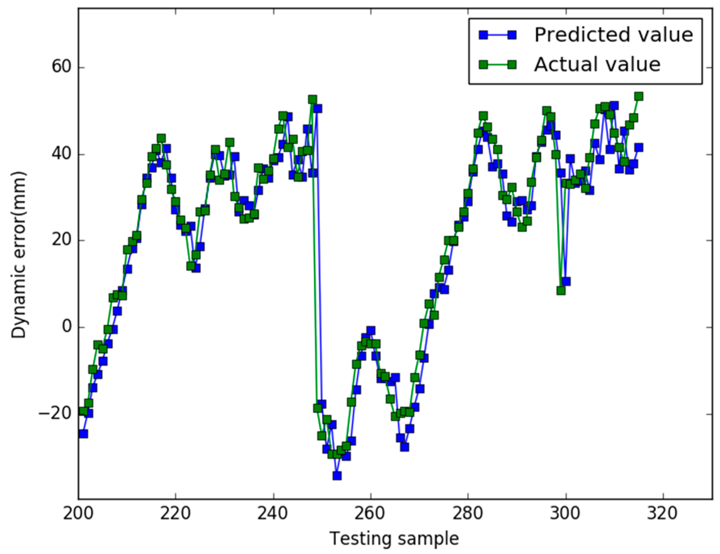
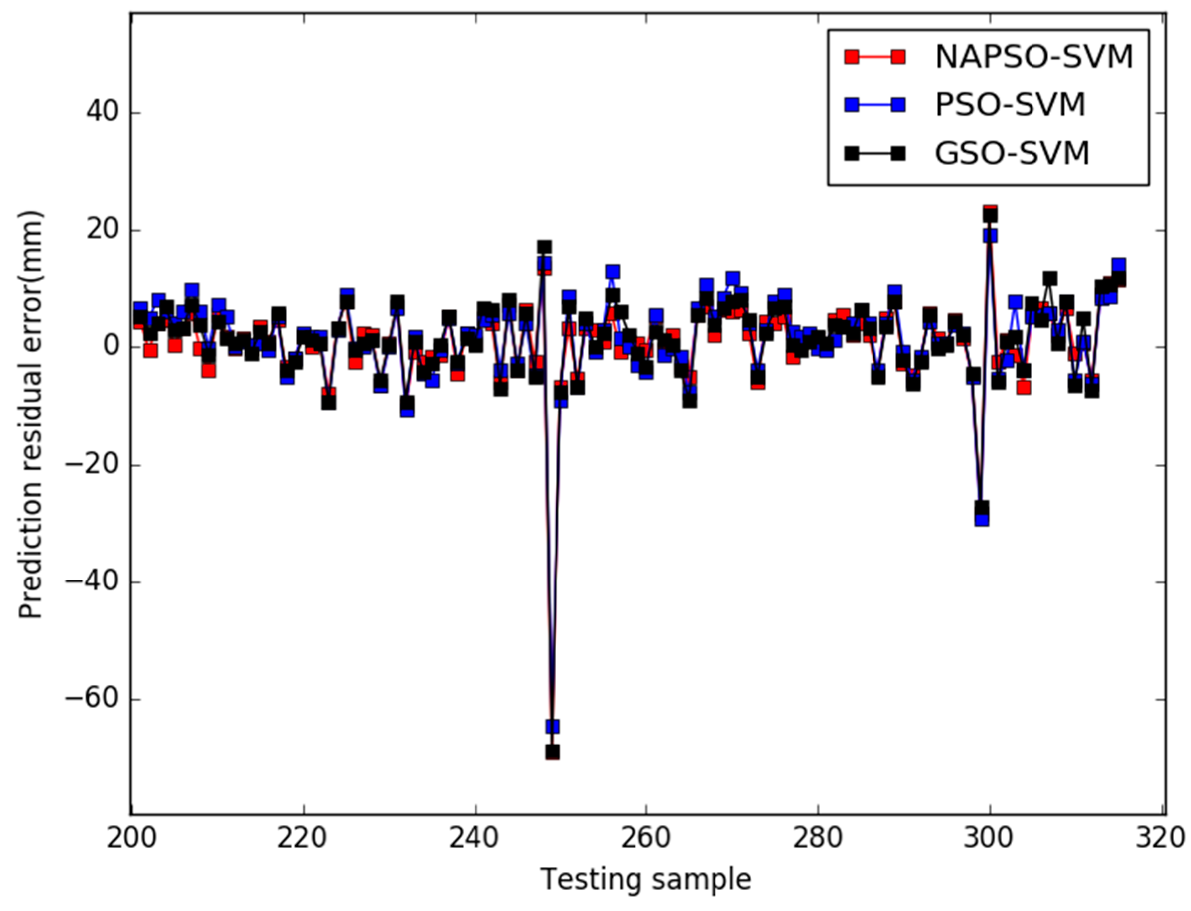
5. Results
6. Conclusions
Acknowledgments
Author Contributions
Conflicts of Interest
References
- Cheng, S.; Cai, Z.; Li, J.; Gao, H. Extracting Kernel Dataset from Big Sensory Data in Wireless Sensor Networks. IEEE Trans. Knowl. Data Eng. 2017, 29, 813–827. [Google Scholar] [CrossRef]
- Jiang, D.; Li, W.; Lv, H. An energy-efficient cooperative multicast routing in multi-hop wireless networks for smart medical applications. Neurocomputing 2017, 220, 160–169. [Google Scholar] [CrossRef]
- Jiang, D.; Wang, Y.; Han, Y.; Lv, H. Maximum connectivity-based channel allocation algorithm in cognitive wireless networks for medical applications. Neurocomputing 2017, 220, 41–51. [Google Scholar] [CrossRef]
- Jiang, D.; Xu, Z.; Li, W.; Yao, C.; Lv, Z.; Li, T. An energy-efficient multicast algorithm with maximum network throughput in multi-hop wireless networks. J. Commun. Netw. 2016, 18, 713–724. [Google Scholar]
- Yakovlev, V.T. Method of Determining Dynamic Measurement Error Due to Oscillographs. Meas. Tech. 1987, 30, 331–334. [Google Scholar] [CrossRef]
- Chen, Y. Area-Efficient Fixed-Width Squarer with Dynamic Error-Compensation Circuit. IEEE Trans. Circuits Syst. II 2015, 62, 851–855. [Google Scholar] [CrossRef]
- Jiang, D.; Nie, L.; Lv, Z.; Song, H. Spatio-temporal Kronecker compressive sensing for traffic matrix recovery. IEEE Access 2016, 4, 3046–3053. [Google Scholar] [CrossRef]
- Yakovlev, V.T.; Collins, E.; Flores, K.; Pershad, P.; Stemkovski, M.; Stephenson, L. Statistical Error Model Comparison for Logistic Growth of Green Algae (Raphidocelis subcapitata). Appl. Math. Lett. 2017, 64, 213–222. [Google Scholar]
- Cheng, S.; Cai, Z.; Li, J.; Fang, X. Drawing Dominant Dataset from Big Sensory Data in Wireless Sensor Networks. In Proceedings of the 34th Annual IEEE International Conference on Computer Communications, Kowloon, Hong Kong, China, 26 April–1 May 2015; pp. 531–539. [Google Scholar]
- Trapero, J.; Kourentzes, N.; Martin, A. Short-term solar irradiation forecasting based on dynamic harmonic regression. Energy 2015, 84, 289–295. [Google Scholar] [CrossRef]
- Yang, H.; Zhang, L.; Zhou, J.; Fei, Y.; Peng, D. Modelling of dynamic measurement error for parasitic time grating sensor based on Bayesian principle. Opt. Precis. Eng. 2015, 24, 2523–2531. [Google Scholar] [CrossRef]
- Ge, L.; Zhao, W.; Zhao, S.; Zhou, J. Novel error prediction method of dynamic measurement lacking information. J. Test. Eval. 2012, 40. [Google Scholar] [CrossRef]
- Jiang, D.; Xu, Z.; Lv, Z. A multicast delivery approach with minimum energy consumption for wireless multi-hop networks. Telecommun. Syst. 2016, 62, 771–782. [Google Scholar] [CrossRef]
- He, Z.; Cai, Z.; Cheng, S.; Wang, X. Approximate Aggregation for Tracking Quantiles and Range Countings in Wireless Sensor Networks. Theor. Comput. Sci. 2015, 607, 381–390. [Google Scholar] [CrossRef]
- Barbounis, T.G.; Theocharis, J.B. A locally recurrent fuzzy neural network with application to the wind speed prediction using spatial correlation. Neurocomputing 2007, 70, 1525–1542. [Google Scholar] [CrossRef]
- Cheng, S.; Cai, Z.; Li, J. Curve Query Processing in Wireless Sensor Networks. IEEE Trans. Veh. Technol. 2015, 64, 5198–5209. [Google Scholar] [CrossRef]
- Sasikala, S.; Balamurugan, S.; Geetha, S. A Novel Memetic Algorithm for Discovering Knowledge in Binary and Multi Class Predictions Based on Support Vector Machine. Appl. Soft Comput. 2016, 49, 407–422. [Google Scholar]
- Malvoni, M.; De Giorgi, M.G.; Congedo, P.M. Photovoltaic Forecast Based on Hybrid PCA–LSSVM Using Dimensionality Reduced Data. Neurocomputing 2016, 211, 72–83. [Google Scholar] [CrossRef]
- Jiang, D.; Xu, Z.; Liu, J.; Zhao, W. An optimization-based robust routing algorithm to energy-efficient networks for cloud computing. Telecommun. Syst. 2016, 63, 89–98. [Google Scholar] [CrossRef]
- Jiang, D.; Zhang, P.; Lv, Z.; Song, H. Energy-efficient multi-constraint routing algorithm with load balancing for smart city applications. IEEE Intern. Things J. 2016, 3, 1437–1447. [Google Scholar] [CrossRef]
- Jiang, D.; Huo, L.; Lv, Z.; Song, H.; Qin, W. A joint multi-criteria utility-based network selection approach for vehicle-to-infrastructure networking. IEEE Trans. Intell. Transp. Syst. 2017. [Google Scholar] [CrossRef]
- Zhong, Y.; Ning, J.; Zhang, H. Multi-agent Simulated Annealing Algorithm based on Particle Swarm Optimisation Algorithm. Int. J. Comput. Appl. Technol. 2012, 43, 335–342. [Google Scholar] [CrossRef]
- Zainal, N.; Zain, A.; Radzi, N. Glowworm Swarm Optimization (GSO) for optimization of machining parameters. J. Intell. Manuf. 2016, 27, 998–1006. [Google Scholar] [CrossRef]
- Lentka, Ł.; Smulko, J.M.; Ionescu, R.; Granqvist, C.G.; Kish, L.B. Determination of gas mixture components using fluctuation enhanced sensing and the LS-SVM regression algorithm. Metrol. Meas. Syst. 2015, 22, 341–350. [Google Scholar] [CrossRef]
- Kennedy, J.; Eberhart, R. Particle Swarm Optimization. In Proceedings of the First IEEE International Conference on Neural Networks, Perth, Australia, 27 November–1 December 1995; pp. 1942–1948. [Google Scholar]
- Li, J.; Cheng, S.; Cai, Z.; Yu, J.; Wang, C.; Li, Y. Approximate Holistic Aggregation in Wireless Sensor Networks. ACM Trans. Sens. Netw. 2017, 13, 11:1–11:24. [Google Scholar] [CrossRef]
- Jiang, M.; Luo, J.; Jiang, D.; Xiong, J.; Song, H.; Shen, J. A Cuckoo Search-support Vector Machine Model for Predicting Dynamic Measurement Errors of Sensors. IEEE Access 2016, 4, 5030–5037. [Google Scholar] [CrossRef]
- Krishnanand, K.N.; Ghose, D. Glowworm swarm optimization for simultaneous capture of multiple local optima of multimodal functions. Swarm Intell. 2009, 3, 87–124. [Google Scholar] [CrossRef]


| Input | Output |
|---|---|
| … | … |
| MODEL | MAPE | RMSE |
|---|---|---|
| NAPSO-SVM | 0.0744 | 0.1879 |
| PSO-SVM | 0.2423 | 0.4710 |
| GSO-SVM | 0.1493 | 0.3128 |
| MODEL | MAPE | RMSE |
|---|---|---|
| NAPSO-SVM | 0.3840 | 0.8015 |
| PSO-SVM | 0.5377 | 0.8209 |
| GSO-SVM | 0.4403 | 0.8356 |
© 2018 by the authors. Licensee MDPI, Basel, Switzerland. This article is an open access article distributed under the terms and conditions of the Creative Commons Attribution (CC BY) license (http://creativecommons.org/licenses/by/4.0/).
Share and Cite
Jiang, M.; Jiang, L.; Jiang, D.; Li, F.; Song, H. A Sensor Dynamic Measurement Error Prediction Model Based on NAPSO-SVM. Sensors 2018, 18, 233. https://doi.org/10.3390/s18010233
Jiang M, Jiang L, Jiang D, Li F, Song H. A Sensor Dynamic Measurement Error Prediction Model Based on NAPSO-SVM. Sensors. 2018; 18(1):233. https://doi.org/10.3390/s18010233
Chicago/Turabian StyleJiang, Minlan, Lan Jiang, Dingde Jiang, Fei Li, and Houbing Song. 2018. "A Sensor Dynamic Measurement Error Prediction Model Based on NAPSO-SVM" Sensors 18, no. 1: 233. https://doi.org/10.3390/s18010233
APA StyleJiang, M., Jiang, L., Jiang, D., Li, F., & Song, H. (2018). A Sensor Dynamic Measurement Error Prediction Model Based on NAPSO-SVM. Sensors, 18(1), 233. https://doi.org/10.3390/s18010233