Inclinometer Assembly Error Calibration and Horizontal Image Correction in Photoelectric Measurement Systems

Abstract
:1. Introduction
2. Related Work and Motivation
- (1)
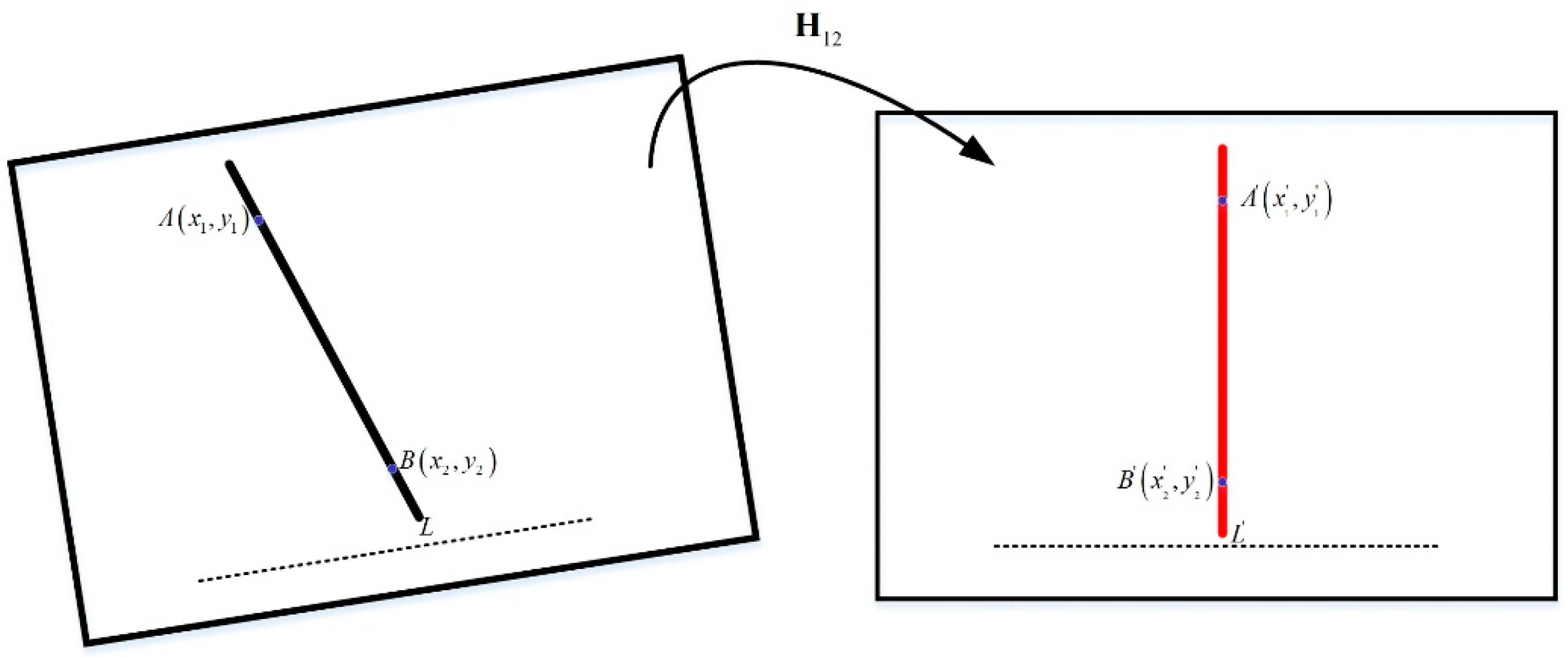
- Based on the principle that “the plumb lines of edges of constructions in the real world should become vertical lines on the image plane after horizontal correction of the attitude of the camera by the inclinometer”, only the angle information of the different attitudes obtained by the inclinometer and the plumb lines in the acquired images are needed to calibrate the inclinometer assembly error matrix in the photoelectric system, which is fast and easy.
- (2)
- The inclinometer assembly error matrix expression in photoelectric systems is analyzed in this paper, and an optimization function to achieve the optimal solution for the assembly error matrix by minimizing the Sum of Squared Residuals (SSR) is established.
- (3)
- A captured image with an arbitrary inclination angle can be horizontally corrected after the system calibration in order to test the correctness of the calibration result.
- (4)
- Factors affecting the accuracy of the calibration results are analyzed by means of a simulation perturbation experiment and a practical experiment, which show sufficient accuracy for the proposed method.
- (5)
- The experimental setup is simple to implement. The calibration process is easily operated. The experimental results are stable and effective.
3. Inclinometer Assembly Error
4. Inclinometer Assembly Error Calibration and Horizontal Image Correction
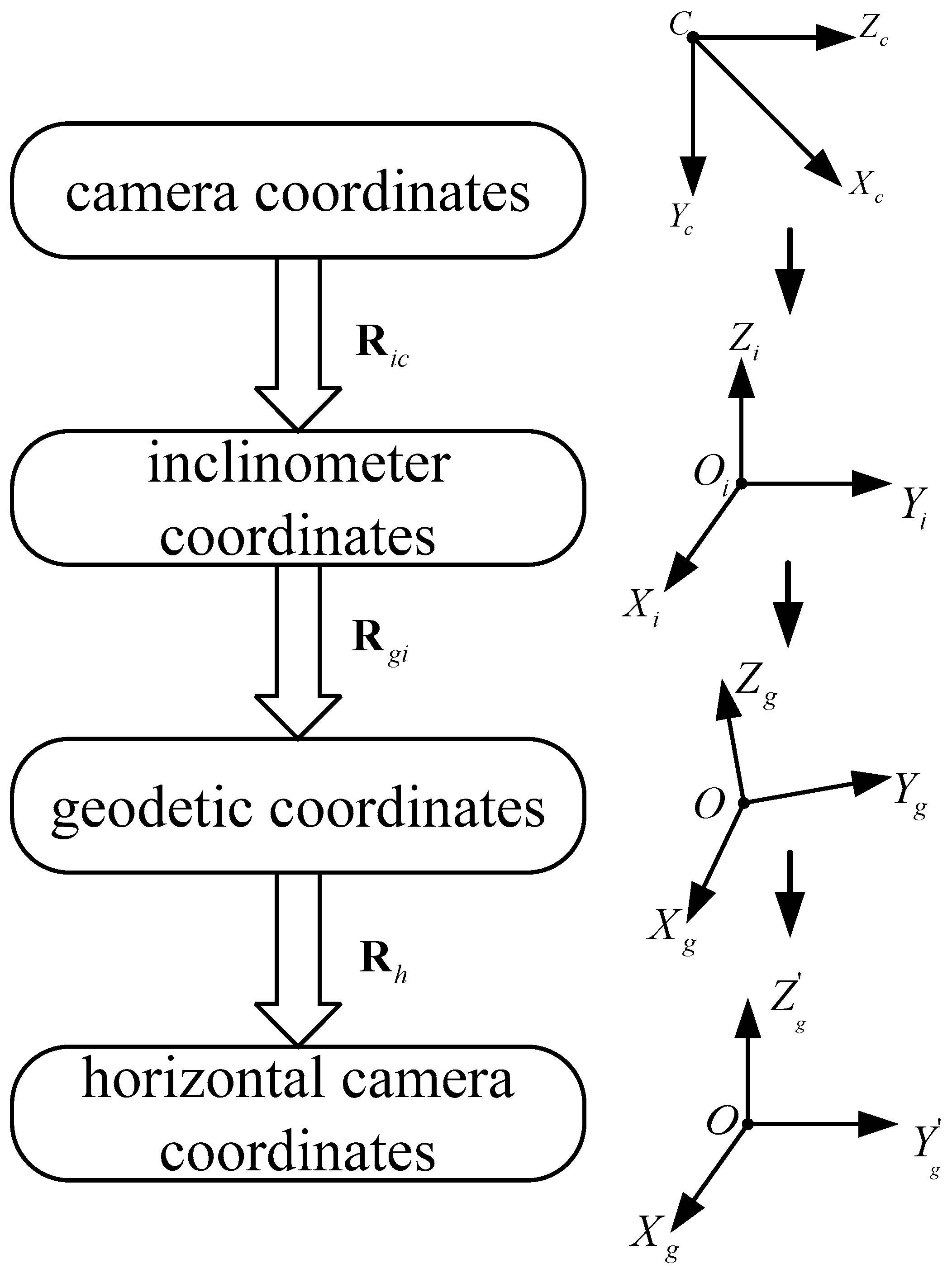
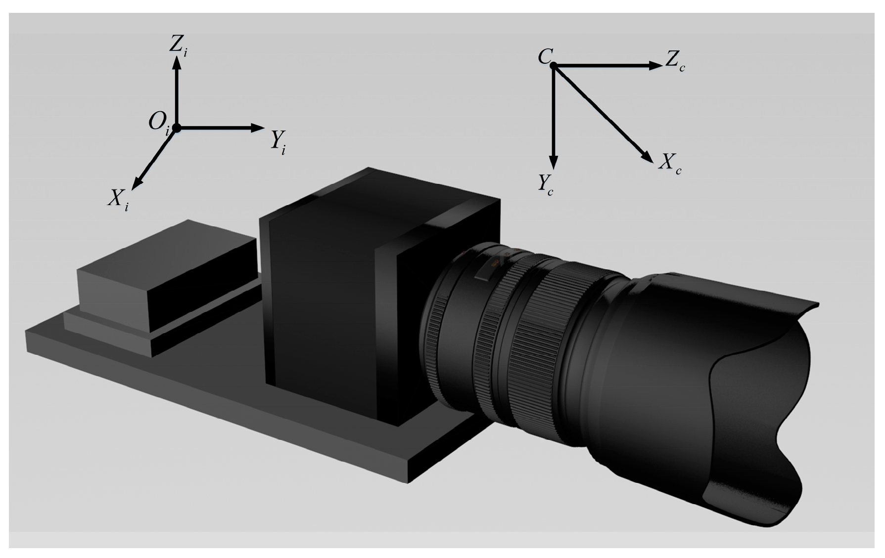
4.1. Relationship between the Geodetic Coordinate System and the Inclinometer Coordinate System
4.2. Horizontal Image Correction Using the Inclinometer
| Algorithm 1: Horizontal image correction using the inclinometer. |
|
4.3. Inclinometer Assembly Error Calibration Based on Plumb Lines
5. Experimental Results and Analyses
5.1. Photoelectric Measurement System
5.2.Calibration of Camera Intrinsic Parameter and Estimation of Lens Radial Distortion Parameter
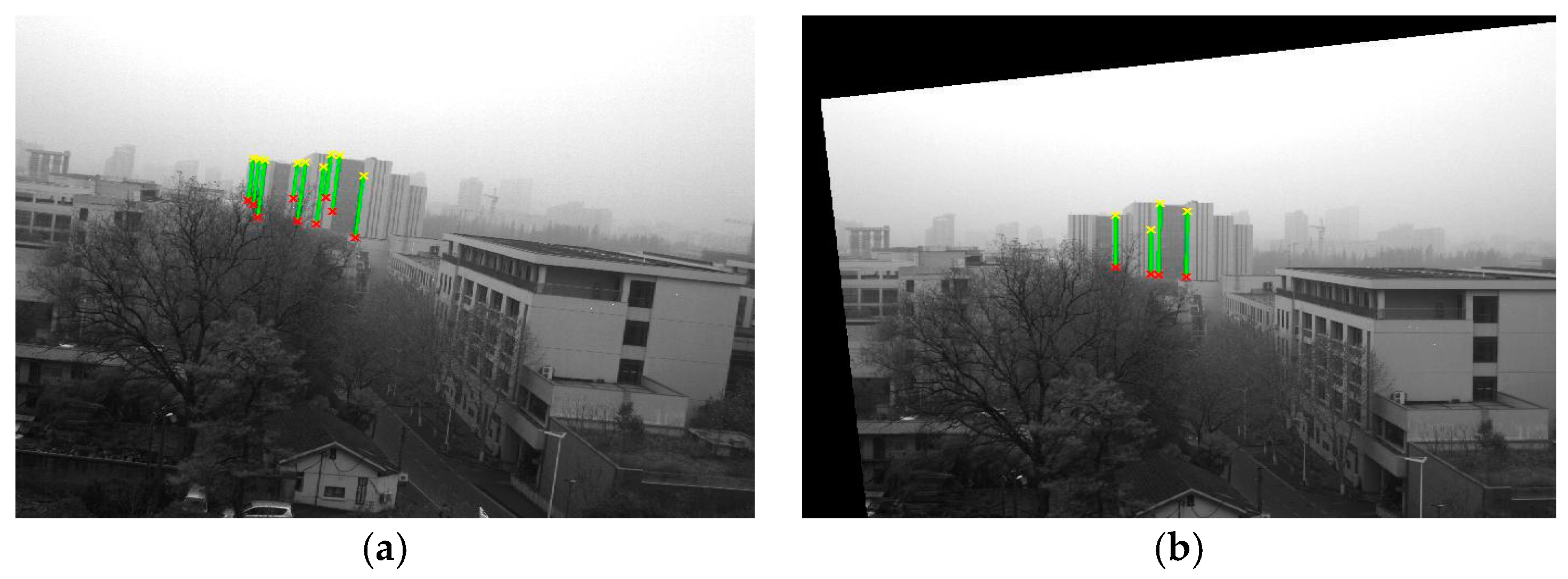
5.3. Experimental Data Measurement
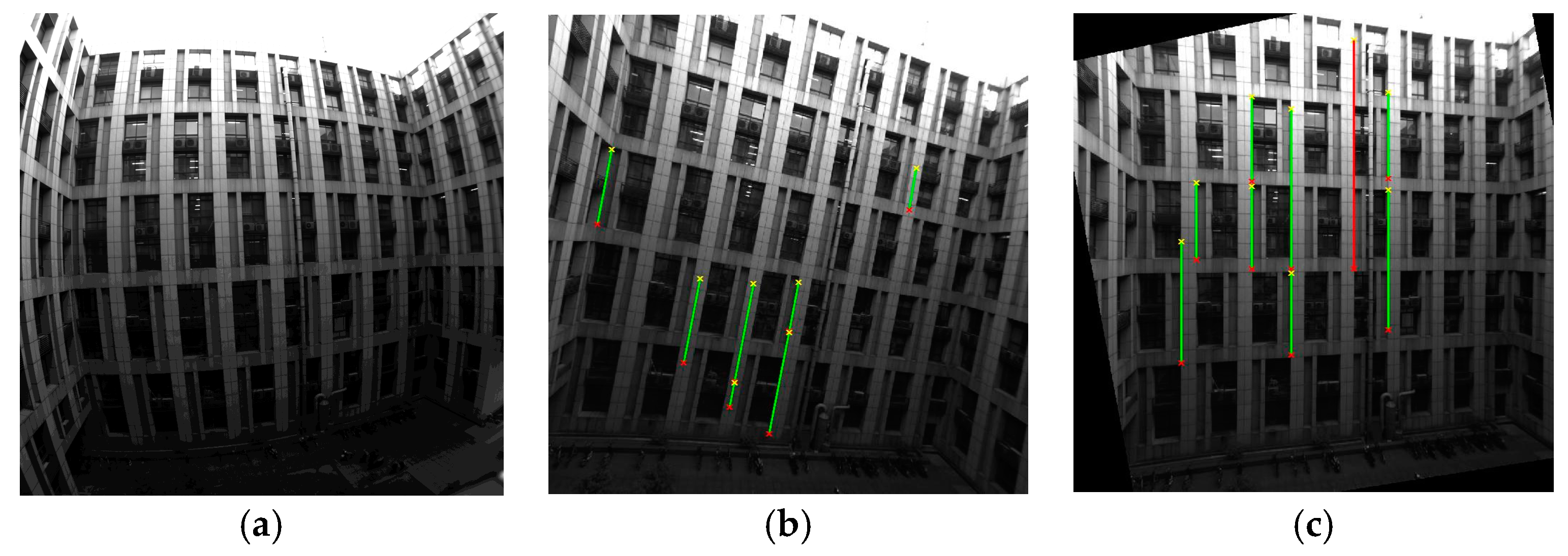
5.4. Inclinometer Assembly Error Calculation and Horizontal Image Correction
5.5. System Error Analyses
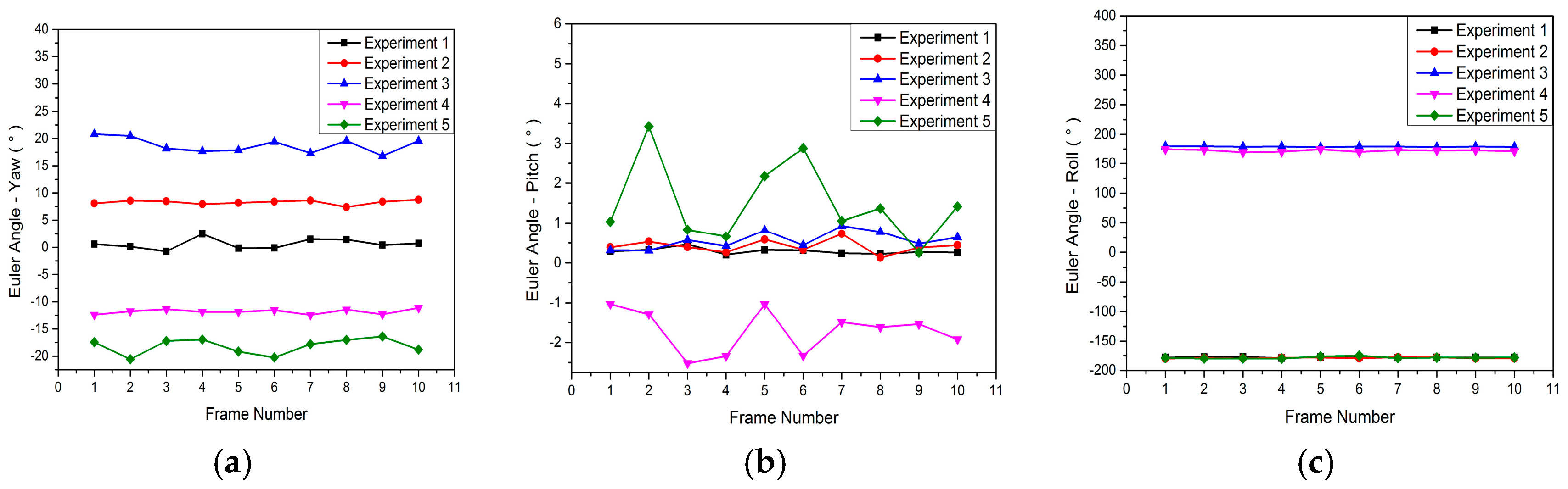
5.5.1. Error Analyses by Simulation Experiment
| Algorithm 2: Pseudocode of the perturbation simulation experiment. |
| For ( is the number of groups in the experiment) For ( is the number of images taken in each group) For ( is the duration over which Gaussian noise was added) (I) Obtain image , and record values of the inclinometer . (II) Detect plumb lines in the image using the Hough line detection method. (III) Add Gaussian noise to the endpoints of detected lines . End End (IV) Calculate the inclinometer assembly error , and decompose the matrix into Euler angles. End (V) Calculate the average of the Euler angles as the final assembly error for each group. (VI) Calculate the mean and the standard deviation of the Euler angle. |
5.5.2. Error Analyses by Practical Experiment
| Algorithm 3: Pseudocode for the practical experiment. |
|
5.6. Comparison with Other Methods
6. Conclusions
Acknowledgments
Author Contributions
Conflicts of Interest
References
- Ma, D.M.; Shiau, J.K.; Wang, I.C.; Lin, Y.H. Attitude Determination Using a MEMS-Based Flight Information Measurement Unit. Sensors 2012, 12, 1–23. [Google Scholar] [CrossRef] [PubMed]
- Nadarajah, N.; Teunissen, P.J.G.; Raziq, N. BeiDou Inter-Satellite-Type Bias Evaluation and Calibration for Mixed Receiver Attitude Determination. Sensors 2013, 13, 9435–9463. [Google Scholar] [CrossRef] [PubMed]
- Cong, L.; Li, E.; Qin, H.; Voon Ling, K.; Xue, R. A Performance Improvement Method for Low-Cost Land Vehicle GPS/MEMS-INS Attitude Determination. Sensors 2015, 15, 5722–5746. [Google Scholar] [CrossRef] [PubMed]
- Antonio, A.; Mark, P.; Giovanni, P. Benefits of Combined GPS/GLONASS with Low-Cost MEMS IMUs for Vehicular Urban Navigation. Sensors 2012, 12, 5134–5158. [Google Scholar]
- Kai-Wei, C.; Trung, D.T.; Liao, J.K.; Lai, Y.C.; Chang, C.C.; Cai, J.M.; Huang, S.C. On-Line Smoothing for an Integrated Navigation System with Low-Cost MEMS Inertial Sensors. Sensors 2012, 12, 17372–17389. [Google Scholar]
- Hao, Q.; Cheng, X.; Kang, J.; Jiang, Y. An Image Stabilization Optical System Using Deformable Freeform Mirrors. Sensors 2015, 15, 1736–1749. [Google Scholar] [CrossRef] [PubMed]
- Sun, T.; Xing, F.; You, Z. Optical System Error Analysis and Calibration Method of High-Accuracy Star Trackers. Sensors 2013, 13, 4598–4623. [Google Scholar] [CrossRef] [PubMed]
- Gao, W.; Zhang, Y.; Wang, J. Research on Initial Alignment and Self-Calibration of Rotary Strapdown Inertial Navigation Systems. Sensors 2015, 15, 3154–3171. [Google Scholar] [CrossRef] [PubMed]
- Xian, Z.; Hu, X.; Lian, J.; Zhang, L.; Cao, J.; Wang, Y.; Ma, T. A novel angle computation and calibration algorithm of bio-inspired sky-light polarization navigation sensor. Sensors 2014, 14, 17068–17088. [Google Scholar] [CrossRef] [PubMed]
- Cozman, F.; Krotkov, E. Robot localization using a computer vision sextant. In Proceedings of the 1995 IEEE International Conference on Robotics and Automation, Nagoya, Japan, 21–27 May 1995; Volume 1, pp. 106–111. [Google Scholar]
- Barbour, N.M. Inertial navigation sensors. Available online: http://www.dtic.mil/dtic/tr/fulltext/u2/a581016.pdf (accessed on 6 November 2017).
- Olivares, A.; Ramírez, J.; Górriz, J.M.; Olivares, G.; Damas, M. Detection of (in) activity Periods in Human Body Motion Using Inertial Sensors: A Comparative Study. Sensors 2012, 12, 5791–5814. [Google Scholar] [CrossRef] [PubMed]
- Beṣdok, E. 3D Vision by Using Calibration Pattern with Inertial Sensor and RBF Neural Networks. Sensors 2009, 9, 4572–4585. [Google Scholar] [CrossRef] [PubMed]
- Balletti, C.; Guerra, F.; Tsioukas, V.; Vernier, P. Calibration of action cameras for photogrammetric purposes. Sensors 2014, 14, 17471–17490. [Google Scholar] [CrossRef] [PubMed]
- Niu, X.; You, L.; Zhang, H.; Wang, Q.; Ban, Y. Fast Thermal Calibration of Low-Grade Inertial Sensors and Inertial Measurement Units. Sensors 2013, 13, 12192–12217. [Google Scholar] [CrossRef] [PubMed]
- Ding, J. Research on Attitude Algorithm Based on Micro Inertial Sensors. Master’s Thesis, Shanghai Jiao Tong University, Shanghai, China, 2013. [Google Scholar]
- Wu, Z.; Sun, Z.; Zhang, W.; Chen, Q. A novel approach for attitude estimation using MEMS inertial sensors. In Proceedings of the 2014 IEEE SENSORS, Valencia, Spain, 2–5 November 2014; pp. 1022–1025. [Google Scholar]
- Liu, X. The Attitude Test Algorithm Based on MEMS Multidimensional Inertial Sensors. Master’s Thesis, Harbin Engineering University, Harbin, China, 2013. [Google Scholar]
- Bonnet, S.; Bassompierre, C.; Godin, C.; Lesecq, S.; Barraud, A. Calibration methods for inertial and magnetic sensors. Sensors Actuators A Phys. 2009, 156, 302–311. [Google Scholar] [CrossRef]
- Hedrich, F.; Frech, J.; Auber, J.; Sandmaier, H.; Wimmer, W.; Lang, W. Micro-machined inclinometer with high sensitivity and very good stability. Sens. Actuators A Phys. 2002, 97–98, 125–130. [Google Scholar]
- Cao, J.; Zhang, L.; Wu, H.; Wang, L.; Miao, L. Analytical approach for measurement of spatial angle with inclination sensor. J. Xian Jiao Tong Univ. 2013, 47, 109–114. [Google Scholar]
- Tong, G.; Wang, T.; Wu, Z.; Li, Z.; Chen, T. Application of high accuracy inclinometer to deformation measurement for vehicular platform. Opt. Precis. Eng. 2010, 18, 1347–1353. [Google Scholar]
- Lambrecht, S.; Nogueira, S.L.; Bortole, M.; Siqueira, A.A.; Terra, M.H.; Rocon, E.; Pons, J.L. Inertial Sensor Error Reduction through Calibration and Sensor Fusion. Sensors 2016, 16, 235. [Google Scholar] [CrossRef] [PubMed]
- Benosman, R.; Kang, S.B. Panoramic Vision, Sensors Theory and Applications. Sensors 2001, 29, 1989–1997. [Google Scholar]
- Merckel, L.; Nishida, T. Solution of the perspective-three-point problem: Calculation from video image by using inclinometers attached to the camera. In Proceedings of the International Conference on Industrial, Engineering, and Other Applications of Applied Intelligent Systems, Kyoto, Japan, 26–29 June 2007; Springer: Berlin/Heidelberg, Germany; pp. 324–333. [Google Scholar]
- Chang, J. Calculation of state parameters of inclinometer in digital zenith camera. Petrochem. Ind. Technol. 2016, 24, 2325–2331. [Google Scholar]
- Hirata, H.; Yagura, C.; Oka, S.; Yoshimura, K.; Hamachi, N.; Tahara, H. Measurement of the Thoracic Kyphosis Angle with a Digital Inclinometer. Rigakuryoho Kagaku 2012, 27, 115–118. [Google Scholar] [CrossRef]
- Hobbs, R.R. Marine Navigation, 3rd ed.; Naval Institute Press: Annapolis, MD, USA, 1974. [Google Scholar]
- Hartley, R.; Zisserman, A. Multiple View Geometry in Computer Vision; Cambridge University Press: Cambridge, UK, 2003. [Google Scholar]
- Rousso, B.; Avidan, S.; Shashua, A.; Peleg, S. Robust Recovery of Camera Rotation from Three Frames. In Proceedings of the CVPR IEEE Computer Society Conference on Computer Vision and Pattern Recognition, San Francisco, CA, USA, 18–20 June 1996; pp. 796–802. [Google Scholar]
- Simon, D.; Simon, D.L. Analytic Confusion Matrix Bounds for Fault Detection and Isolation Using a Sum-of-squared-residuals Approach. IEEE Trans. Reliab. 2010, 59, 287–296. [Google Scholar] [CrossRef]
- Ballard, D.H. Generalizing the Hough transform to detect arbitrary shapes. Pattern Recognit. 1981, 13, 111–122. [Google Scholar] [CrossRef]
- Bertsekas, D.P. Nonlinear programming. J. Oper. Res. Soc. 1997, 48, 334. [Google Scholar] [CrossRef]
- Stewart, G.W.; Sun, J. Matrix Perturbation Theory; Academic Press: Cambridge, MA, USA, 1990. [Google Scholar]
- Strand, R.; Hayman, E. Correcting Radial Distortion by Circle Fitting. In Proceedings of the British Machine Vision Conference, Oxford, UK, 5–8 September 2005. [Google Scholar]
- Tsai, R.Y. A versatile camera calibration technique for high-accuracy 3D machine vision metrology using off-the-shelf TV cameras and lenses. IEEE J. Robot. Autom. 2003, 3, 323–344. [Google Scholar] [CrossRef]
- Zhang, Z. Flexible camera calibration by viewing a plane from unknown orientations. In Proceedings of the Seventh IEEE International Conference on Computer Vision, Kerkyra, Greece, 20–27 September 1999; pp. 666–673. [Google Scholar]
- Pio, R.L. Euler angle transformations. IEEE Trans. Autom. Control 1967, 11, 707–715. [Google Scholar] [CrossRef]
- Wang, H.; Leng, Y.; Wang, Z.; Wu, X. Application of image correction and bit-plane fusion in generalized PCA based face recognition. Pattern Recognit. Lett. 2007, 28, 2352–2358. [Google Scholar] [CrossRef]
- Zafarifar, B.; Weda, H.; With, P.H.N.D. Horizon detection based on sky-color and edge features. In Proceedings of the SPIE—The International Society for Optical Engineering, San Jose, CA, USA, 27–31 January 2008. [Google Scholar]
- Chen, L.; Li, X.; Lu, L. Research and modification of license plate tilt correction algorithm. Comput. Mod. 2013, 12, 91–97. [Google Scholar]
- Zisserman, A. Geometric Framework for Vision I: Single View and Two-View Geometry; Cambridge University Press: Cambridge, UK, 1997. [Google Scholar]
- Criminisi, A.; Reid, I.; Zisserman, A. A plane measuring device. Image Vis. Comput. 1999, 17, 625–634. [Google Scholar] [CrossRef]


| Camera Parameter | Value |
|---|---|
| Resolution | 4090 × 3072 |
| Pixel size | 5.5 μm × 5.5 μm |
| Device dimension | 22.5 mm 16.9 mm |
| Focal length | 35 mm |
| Frame frequency | 64 fps |
| angular resolution | 0.16 mrad |
| Camera Parameter | Value |
|---|---|
| Resolution | 2048 × 2048 |
| Pixel size | 5.5 μm × 5.5 μm |
| Device dimension | 11.3 mm 11.3 mm |
| Focal length | 8 mm |
| Frame frequency | 25 fps |
| angular resolution | 4 MP |
| (a) Inclination Data in System 1 (°) | |||||
| No. | -axis Inclination | -axis Inclination | No. | -axis Inclination | -axis Inclination |
| 1 | 1°41′21″ | −0°26′12″ | 7 | 0°44′33″ | −0°14′51″ |
| 2 | 7°15′8″ | 2°48′38″ | 8 | −2°53′53″ | −6°11′21″ |
| 3 | −5°36′24″ | −6°37′34″ | 9 | −6°20′5″ | −0°41′4″ |
| 4 | 1°14′16″ | 4°16′53″ | 10 | −6°36′41″ | −6°26′12″ |
| 5 | −0°21′50″ | −6°16′36″ | 11 | 3°42′48″ | −7°30′0″ |
| 6 | 5°7′34″ | −3°24′27″ | 12 | 3°51′33″ | 4°59′42″ |
| (b) Inclination Data in System 2 (°) | |||||
| No. | -axis Inclination | -axis Inclination | No. | -axis Inclination | -axis Inclination |
| 1 | 0.01 | −0.03 | 10 | −1.53 | −5.75 |
| 2 | −3.15 | −1.94 | 11 | −4.54 | −6.57 |
| 3 | −1.53 | −1.43 | 12 | 6.12 | −6.88 |
| 4 | 1.78 | −0.20 | 13 | 2.18 | −5.05 |
| 5 | 2.94 | −0.26 | 14 | −0.42 | 5.77 |
| 6 | 4.09 | −0.59 | 15 | 3.05 | 3.25 |
| 7 | 5.75 | −0.28 | 16 | −2.00 | 4.07 |
| 8 | 7.56 | −0.57 | 17 | −0.04 | 2.95 |
| 9 | −9.36 | −1.85 | 18 | 0.75 | 0.89 |
| Line No. | Before Horizontal Correction | After Horizontal Correction | ||||
|---|---|---|---|---|---|---|
| Starting Point | End Point | Angle (°) | Starting Point | End Point | Angle (°) | |
| 1 | (1043, 1116) | (1004, 1321) | −76.30 | (1247, 334) | (1247, 518) | 90 |
| 2 | (1003, 1326) | (920, 1749) | −78.89 | (1392, 133) | (1392, 239) | 90 |
| 3 | (1534, 640) | (1503, 816) | −80.01 | (1115, 423) | (1115, 667) | 90 |
| 4 | (855, 1124) | (776, 1531) | −79.02 | (1588, 133) | (1588, 402) | 90 |
| 5 | (775, 1536) | (755, 1639) | −79.01 | (381, 485) | (382, 599) | 89.50 |
| 6 | (632, 1103) | (564, 1453) | −79.00 | (303, 134) | (303, 357) | 90 |
| 7 | (263, 564) | (203, 875) | −79.08 | (248, 117) | (248, 235) | 90 |
| (a) Mean of the Euler Angles | |||
| No. | Yaw | Pitch | Roll |
| 1 | 0.6415 | 0.2888 | −178.0544 |
| 2 | 8.2894 | 0.4158 | −178.0544 |
| 3 | 18.7872 | 0.5699 | 179.2778 |
| 4 | −11.8215 | −1.7134 | 172.4610 |
| 5 | −18.1659 | 1.5106 | −178.4386 |
| (b) Standard Deviation of the Euler Angles | |||
| No. | Yaw | Pitch | Roll |
| 1 | 0.9574 | 0.0731 | 0.5204 |
| 2 | 0.4007 | 0.1694 | 0.8484 |
| 3 | 1.3761 | 0.2176 | 0.6053 |
| 4 | 0.4516 | 0.5442 | 1.8206 |
| 5 | 1.4514 | 1.0103 | 1.5745 |
| AVE | 0.9276 | 0.4029 | 1.0732 |
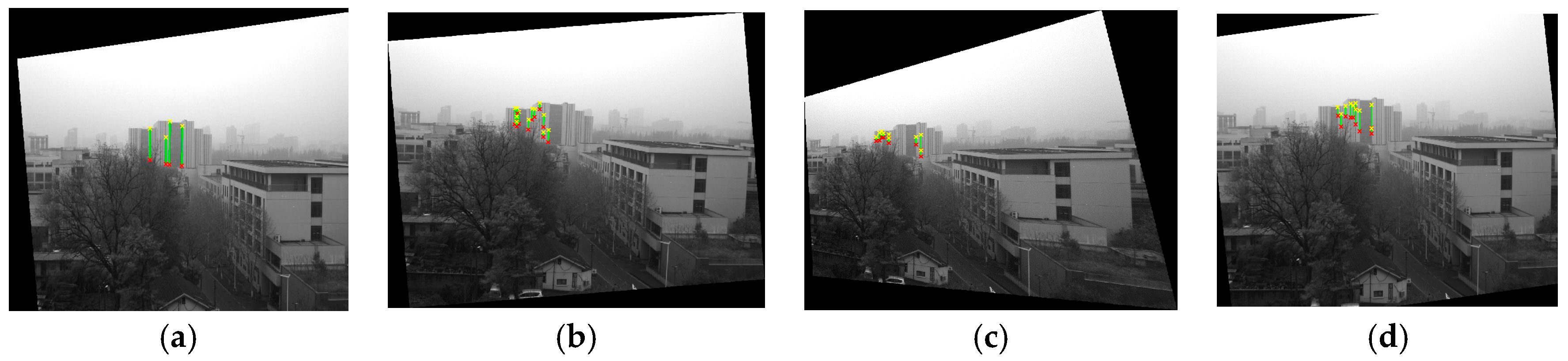
| (a) Image (a) | ||||||
| Line No. | Before Horizontal Correction | After Horizontal Correction | ||||
| Starting Point | End Point | Angle (°) | Starting Point | End Point | Angle (°) | |
| 1 | (1345, 1043) | (1327, 1169) | -81.87 | (1511, 1093) | (1510, 1185) | 89.38 |
| 2 | (1564, 1031) | (1544, 1162) | -81.32 | (1457, 1006) | (1457, 1120) | 90 |
| 3 | (1194, 1025) | (1178, 1137) | -80.37 | (1737, 1258) | (1737, 1359) | 90 |
| 4 | (1135, 1042) | (1123, 1125) | -81.77 | (1533, 1269) | (1533, 1357) | 90 |
| 5 | (1615, 1016) | (1589, 1185) | -81.25 | (1735, 1374) | (1735, 1461) | 90 |
| 6 | (1519, 1134) | (1501, 1248) | -81.03 | (1127, 1160) | (1127, 1348) | 90 |
| (b) Image (b) | ||||||
| Line No. | Before Horizontal Correction | After Horizontal Correction | ||||
| Starting Point | End Point | Angle (°) | Starting Point | End Point | Angle (°) | |
| 1 | (1646, 940) | (1710, 1348) | 81.09 | (1827, 1250) | (1827, 1537) | 90 |
| 2 | (1630, 1004) | (1642, 1085) | 81.57 | (1864, 1108) | (1864, 1246) | 90 |
| 3 | (1643, 1090) | (1663, 1213) | 80.76 | (1864, 1252) | (1864, 1348) | 90 |
| 4 | (1336, 1063) | (1366, 1254) | 81.07 | (1912, 1156) | (1912, 1399) | 90 |
| 5 | (1762, 1070) | (1785, 1221) | 81.34 | (2056, 1319) | (2056, 1566) | 90 |
| 6 | (1787, 1232) | (1807, 1359) | 81.05 | (1458, 1319) | (1458, 1427) | 90 |
| 7 | (1717, 1138]) | (1738, 1272) | 81.09 | (1801, 1258) | (1801, 1416) | 90 |
| 8 | (1739, 1277) | (1753, 1370) | 81.44 | (1510, 1374) | (1510, 1470) | 90 |
| 9 | (1801, 1010) | (1836, 1236) | 81.19 | (1771, 1307) | (1771, 1484) | 90 |
| 10 | (1369, 1058) | (1384, 1153) | 81.03 | (1487, 1184) | (1487, 1292) | 90 |
| (c) Image (c) | ||||||
| Line No. | Before Horizontal Correction | After Horizontal Correction | ||||
| Starting Point | End Point | Angle (°) | Starting Point | End Point | Angle (°) | |
| 1 | (1941, 1036) | (2017, 1470) | 80.07 | (2284, 1350) | (2284, 1402) | 90 |
| 2 | (1966, 1032) | (2001, 1232) | 80.07 | (2285, 1408) | (2285, 1464) | 90 |
| 3 | (2005, 1254) | (2041, 1463) | 80.23 | (1998, 1296) | (1998, 1352) | 90 |
| 4 | (2173, 998) | (2235, 1353) | 80.09 | (2027, 1181) | (2027, 1237) | 90 |
| 5 | (1886, 1047) | (1948, 1402) | 80.09 | (2030, 1353) | (2030, 1409) | 90 |
| 6 | (2050, 1158) | (2092, 1400) | 80.15 | (2081, 1409) | (2081, 1466) | 90 |
| 7 | (1580, 1179) | (1598, 1282) | 80.09 | (1675, 1356) | (1675, 1412) | 90 |
| 8 | (1599, 1287) | (1620, 1407) | 80.07 | (1707, 1298) | (1707, 1350) | 90 |
| 9 | (1878, 1150) | (1902, 1290) | 80.27 | (1708, 1355) | (1708, 1412) | 90 |
| 10 | (1634, 1166) | (1675, 1401) | 80.23 | (1774, 1355) | (1774, 1411) | 90 |
| 11 | (1677, 1159) | (1725, 1433) | 80.06 | (2056, 1410) | (2056, 1466) | 90 |
| 12 | (1934, 1143) | (1967, 1331) | 80.04 | (2142, 1466) | (2142, 1522) | 90 |
| Method | Proposed Method | PCA Method | Hough Method | Radon Method |
|---|---|---|---|---|
| Computation time (s) | 7.6137 | 35.3295 | 561.3933 | 9.3188 |
| Correction error (pixel) | 0.50 | 3.00 | 0.77 | 0.91 |
© 2018 by the authors. Licensee MDPI, Basel, Switzerland. This article is an open access article distributed under the terms and conditions of the Creative Commons Attribution (CC BY) license (http://creativecommons.org/licenses/by/4.0/).
Share and Cite
Kong, X.; Chen, Q.; Wang, J.; Gu, G.; Wang, P.; Qian, W.; Ren, K.; Miao, X. Inclinometer Assembly Error Calibration and Horizontal Image Correction in Photoelectric Measurement Systems. Sensors 2018, 18, 248. https://doi.org/10.3390/s18010248
Kong X, Chen Q, Wang J, Gu G, Wang P, Qian W, Ren K, Miao X. Inclinometer Assembly Error Calibration and Horizontal Image Correction in Photoelectric Measurement Systems. Sensors. 2018; 18(1):248. https://doi.org/10.3390/s18010248
Chicago/Turabian StyleKong, Xiaofang, Qian Chen, Jiajie Wang, Guohua Gu, Pengcheng Wang, Weixian Qian, Kan Ren, and Xiaotao Miao. 2018. "Inclinometer Assembly Error Calibration and Horizontal Image Correction in Photoelectric Measurement Systems" Sensors 18, no. 1: 248. https://doi.org/10.3390/s18010248