Field Distortion and Optimization of a Vapor Cell in Rydberg Atom-Based Radio-Frequency Electric Field Measurement

 , , ,
, , ,
Abstract
:1. Introduction
2. Theory and Methods
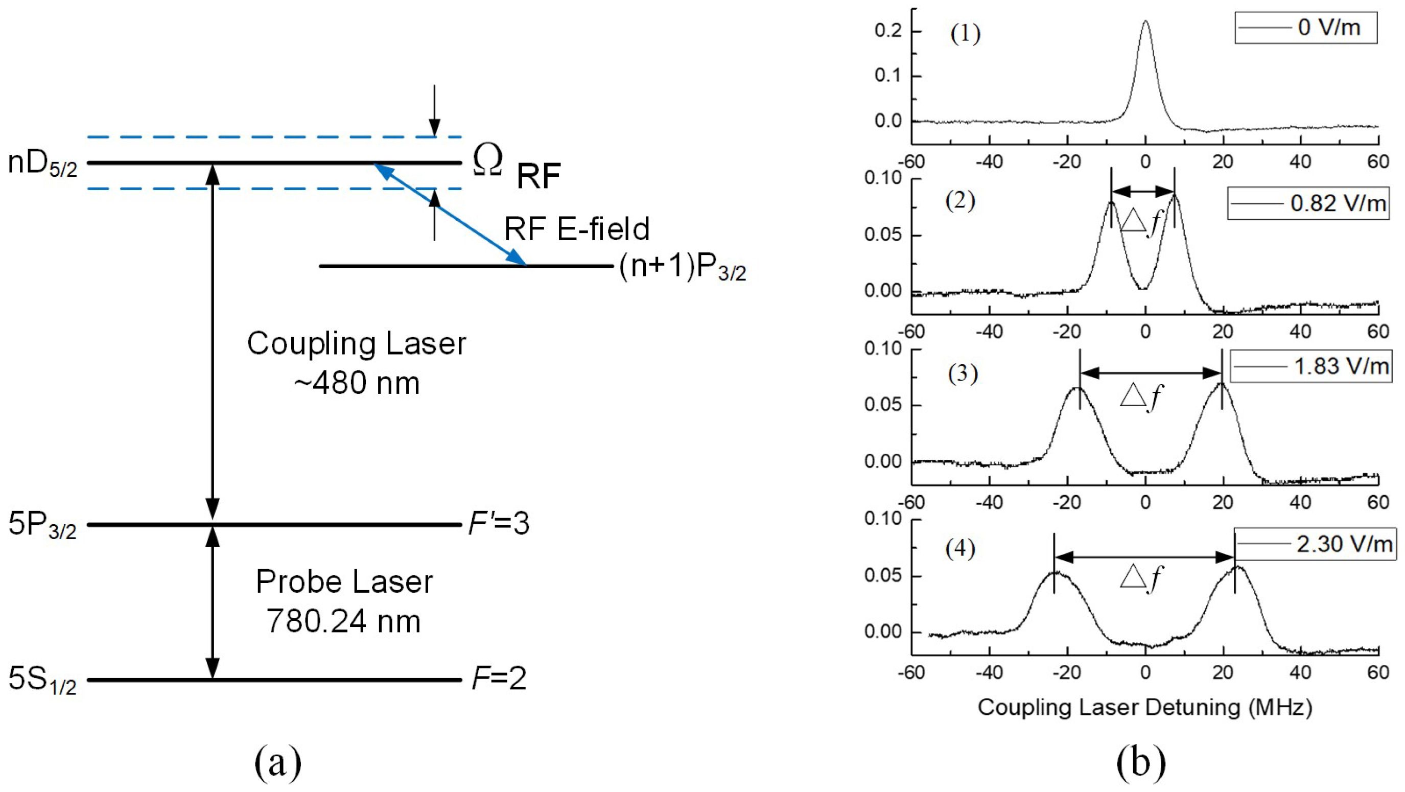
2.1. Quantum-Based RF E-Field Sensing
2.2. Experiment Apparatus and Configuration
3. Results
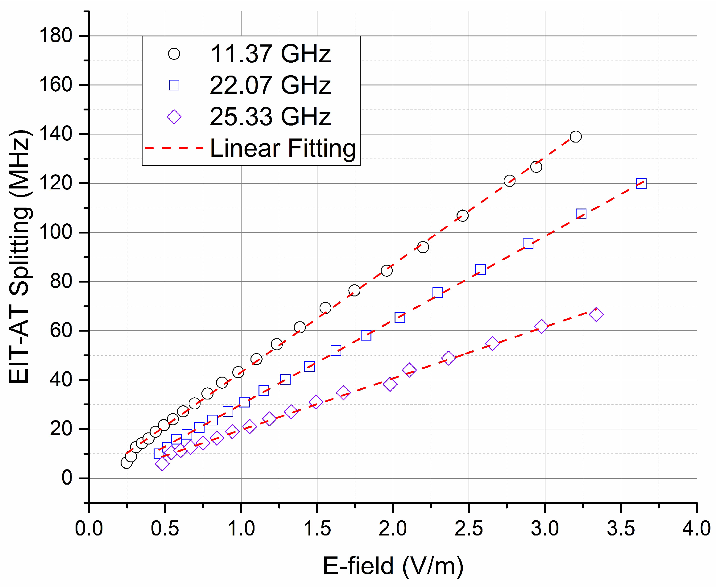
3.1. E-Field Strength Disturbance
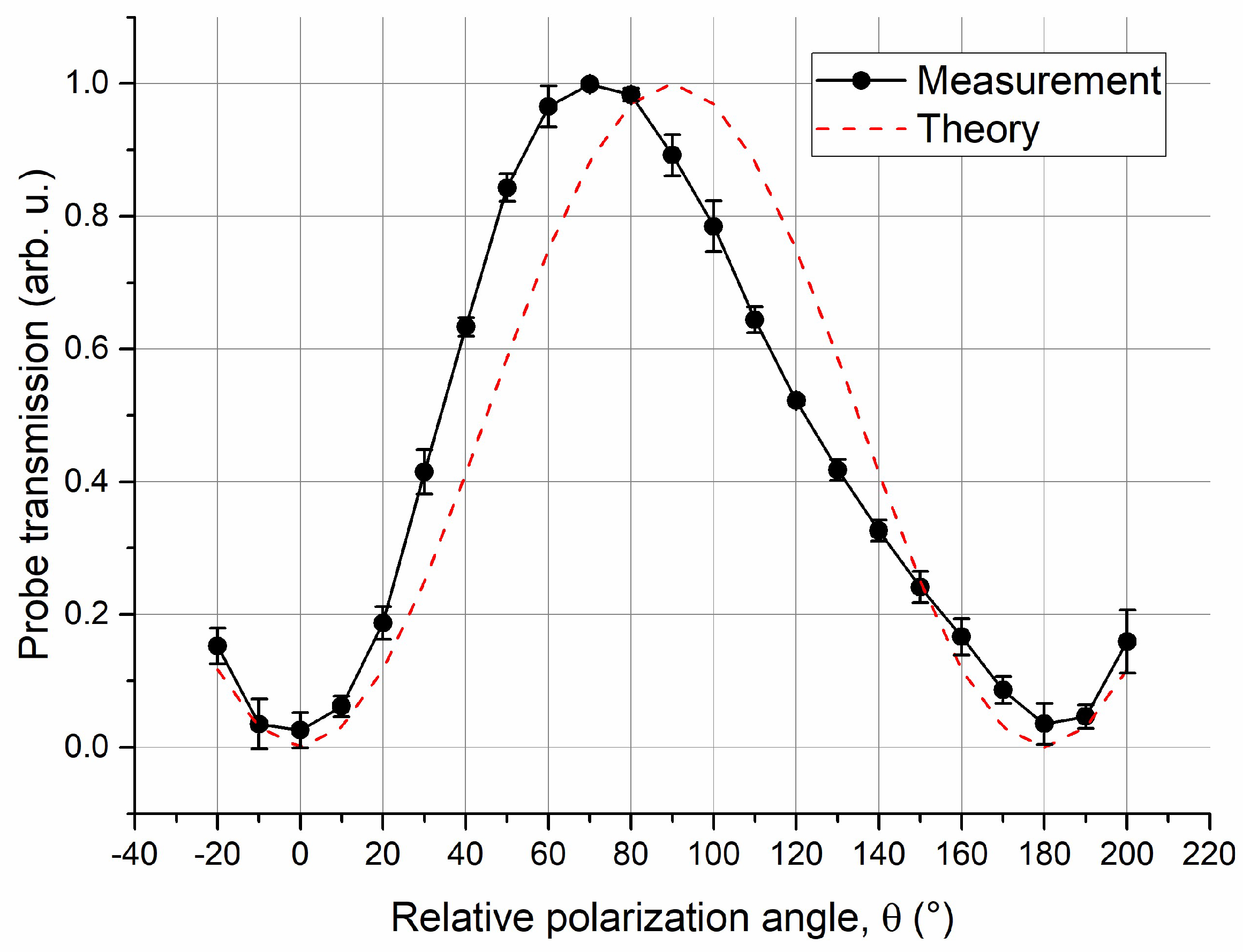
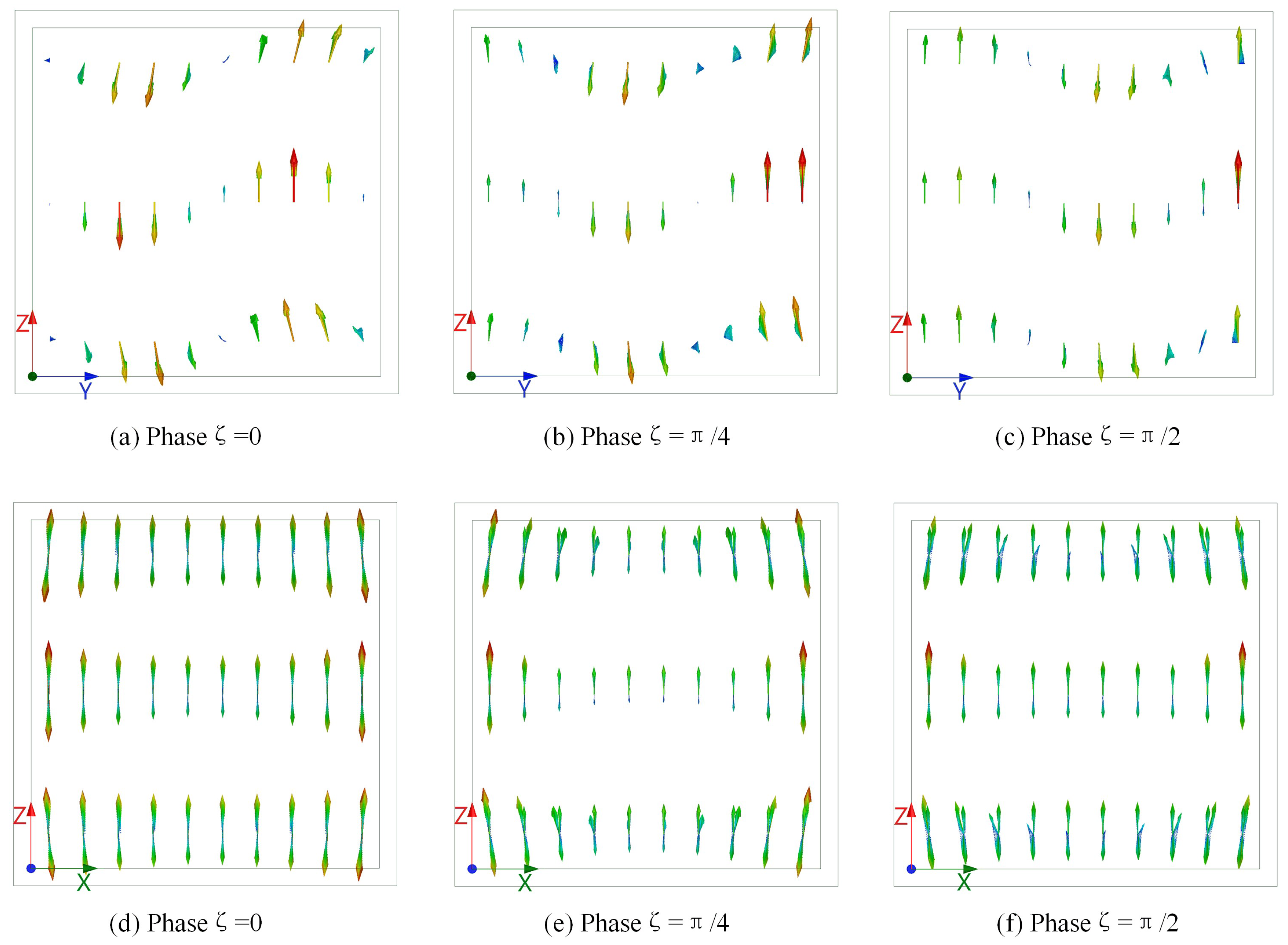
3.2. E-Field Polarization Disturbance
4. Conclusions
Author Contributions
Funding
Acknowledgments
Conflicts of Interest
References
- Degen, C.L.; Reinhard, F.; Cappellaro, P. Quantum Sensing. Rev. Mod. Phys. 2017, 89, 1–39. [Google Scholar] [CrossRef]
- Kitching, J.; Knappe, S.; Donley, E.A. Atomic Sensors—A Review. IEEE Sens. J. 2011, 11, 1749–1758. [Google Scholar] [CrossRef]
- Gallagher, T.F. Rydberg Atoms; Cambridge University Press: Cambridge, UK, 1994; ISBN 9788578110796. [Google Scholar]
- Saffman, M.; Walker, T.G.; Mølmer, K. Quantum information with Rydberg atoms. Rev. Mod. Phys. 2010, 82, 2313–2363. [Google Scholar] [CrossRef] [Green Version]
- Boller, K.; Imamolu, A.; Harris, S. Observation of electromagnetically induced transparency. Phys. Rev. Lett. 1991, 66, 2593–2596. [Google Scholar] [CrossRef] [PubMed]
- Harris, S.E. Eletromagnetically Induced Transparency. Phys. Today 1997, 50, 36–42. [Google Scholar] [CrossRef]
- Autler, S.H.; Townes, C.H. Stark effect in rapidly varying fields. Phys. Rev. 1955, 100, 703–722. [Google Scholar] [CrossRef]
- Sedlacek, J.A.; Schwettmann, A.; Kübler, H.; Löw, R.; Pfau, T.; Shaffer, J.P. Microwave electrometry with Rydberg atoms in a vapour cell using bright atomic resonances. Nat. Phys. 2012, 8, 819–824. [Google Scholar] [CrossRef]
- Sedlacek, J.A.; Schwettmann, A.; Kübler, H.; Shaffer, J.P. Atom-based vector microwave electrometry using rubidium rydberg atoms in a vapor cell. Phys. Rev. Lett. 2013, 111, 063001. [Google Scholar] [CrossRef] [PubMed]
- Holloway, C.L.; Gordon, J.A.; Jefferts, S.; Schwarzkopf, A.; Anderson, D.A.; Miller, S.A.; Thaicharoen, N.; Raithel, G. Broadband Rydberg atom-based electric-field probe for SI-traceable, self-calibrated measurements. IEEE Trans. Antennas Propag. 2014, 62, 6169–6182. [Google Scholar] [CrossRef]
- IEEE. IEEE Standard for Calibration of Electromagnetic Field Sensors and Probes, Excluding Antennas, From 9 kHz to 40 GHz; IEEE Std. 1309-2005; IEEE: Piscataway, NJ, USA, 2013. [Google Scholar] [CrossRef]
- Fan, H.; Kumar, S.; Sedlacek, J.; Kübler, H.; Karimkashi, S.; Shaffer, J.P. Atom based RF electric field sensing. J. Phys. B At. Mol. Opt. Phys. 2015, 48, 202001. [Google Scholar] [CrossRef] [Green Version]
- Kumar, S.; Fan, H.; Kübler, H.; Sheng, J.; Shaffer, J.P. Atom-Based Sensing of Weak Radio Frequency Electric Fields Using Homodyne Readout. Sci. Rep. 2017, 7, 42981. [Google Scholar] [CrossRef] [PubMed] [Green Version]
- Fan, H.Q.; Kumar, S.; Daschner, R.; Kübler, H.; Shaffer, J.P. Subwavelength microwave electric-field imaging using Rydberg atoms inside atomic vapor cells. Opt. Lett. 2014, 39, 3030. [Google Scholar] [CrossRef] [PubMed] [Green Version]
- Holloway, C.L.; Gordon, J.A.; Schwarzkopf, A.; Anderson, D.A.; Miller, S.A.; Thaicharoen, N.; Raithel, G. Sub-wavelength imaging and field mapping via electromagnetically induced transparency and Autler-Townes splitting in Rydberg atoms. Appl. Phys. Lett. 2014, 104, 244102. [Google Scholar] [CrossRef] [Green Version]
- Wade, C.G.; Šibali, N.; De Melo, N.R.; Kondo, J.M.; Adams, C.S.; Weatherill, K.J. Real-time near-field terahertz imaging with atomic optical fluorescence. Nat. Photonics 2017, 11, 40–43. [Google Scholar] [CrossRef]
- Kübler, H.; Shaffer, J.P.; Baluktsian, T.; Löw, R.; Pfau, T. Coherent excitation of Rydberg atoms in micrometre-sized atomic vapour cells. Nat. Photonics 2010, 4, 112–116. [Google Scholar] [CrossRef] [Green Version]
- Epple, G.; Kleinbach, K.S.; Euser, T.G.; Joly, N.Y.; Pfau, T.; Russell, P.S.J.; Löw, R. Rydberg atoms in hollow-core photonic crystal fibres. Nat. Commun. 2014, 5, 4132. [Google Scholar] [CrossRef] [PubMed]
- Simons, M.T.; Gordon, J.A.; Holloway, C.L. Fiber-coupled vapor cell for a portable Rydberg atom-based radio frequency electric field sensor. Appl. Opt. 2018, 57, 6456–6460. [Google Scholar] [CrossRef] [PubMed]
- Holloway, C.L.; Simons, M.T.; Gordon, J.A.; Dienstfrey, A.; Anderson, D.A.; Raithel, G. Electric field metrology for SI traceability: Systematic measurement uncertainties in electromagnetically induced transparency in atomic vapor. J. Appl. Phys. 2017, 121, 233106. [Google Scholar] [CrossRef] [Green Version]
- Fan, H.; Kumar, S.; Sheng, J.; Shaffer, J.P.; Holloway, C.L.; Gordon, J.A. Effect of Vapor-Cell Geometry on Rydberg-Atom-Based Measurements of Radio-Frequency Electric Fields. Phys. Rev. Appl. 2015, 4, 044015. [Google Scholar] [CrossRef]
- Song, Z.; Feng, Z.; Liu, X.; Li, D.; Zhang, H.; Liu, J.; Zhang, L. Quantum-Based Determination of Antenna Finite Range Gain by Using Rydberg Atoms. IEEE Antennas Wirel. Propag. Lett. 2017, 16, 1589–1592. [Google Scholar] [CrossRef]
- Mohr, P.J.; Newell, D.B.; Taylor, B.N.; Tiesinga, E. Data and analysis for the CODATA 2017 special fundamental constants adjustment. Metrologia 2018, 55, 125–146. [Google Scholar] [CrossRef] [Green Version]
- Simons, M.T.; Gordon, J.A.; Holloway, C.L.; Anderson, D.A.; Miller, S.A.; Raithel, G. Using frequency detuning to improve the sensitivity of electric field measurements via electromagnetically induced transparency and Autler-Townes splitting in Rydberg atoms. Appl. Phys. Lett. 2016, 108, 174101. [Google Scholar] [CrossRef]
- Anderson, D.A.; Schwarzkopf, A.; Miller, S.A.; Thaicharoen, N.; Raithel, G.; Gordon, J.A.; Holloway, C.L. Two-photon microwave transitions and strong-field effects in a room-temperature Rydberg-atom gas. Phys. Rev. A 2014, 90, 043419. [Google Scholar] [CrossRef]
- Song, Z.; Liu, X.; Zhang, L.; Zhang, H.; Zhao, J. Quantum based RF E-field sensing by using two-photon transition in Rydberg atoms. In Proceedings of the 2016 Conference on Precision Electromagnetic Measurements (CPEM 2016), Ottawa, ON, Canada, 10–15 July 2016; pp. 2–3. [Google Scholar]
- Simons, M.T.; Gordon, J.A.; Holloway, C.L. Simultaneous use of Cs and Rb Rydberg atoms for dipole moment assessment and RF electric field measurements via electromagnetically induced transparency. J. Appl. Phys. 2016, 120, 123103. [Google Scholar] [CrossRef] [Green Version]
- Mhaskar, R.; Knappe, S.; Kitching, J. A low-power, high-sensitivity micromachined optical magnetometer. Appl. Phys. Lett. 2012, 101, 241105. [Google Scholar] [CrossRef]


| Conventional Probe [11] (Dipole Antenna-Based) | Quantum Sensor | |
|---|---|---|
| Frequency range | <100 GHz | ~1–500 GHz (single sensor) [10] |
| Sensitivity | ~10−1 V/m | ~10−10 V/m (quantum limit) [12,13] |
| Uncertainty | 5–10% (0.5–1 dB) | 0.5% (potentially) [8] |
| Spatial resolution | ~λ/2 | ~λ/100 [14,15,16] |
| Physical dimension | Relatively large, frequency-dependent | Chip-scale, micro vapor cells [17,18,19] |
| Calibration | Needs calibration in a standard RF E-field | Self-calibrated [10] |
| Traceability | Complex | Clear, linking to Planck’s constant |
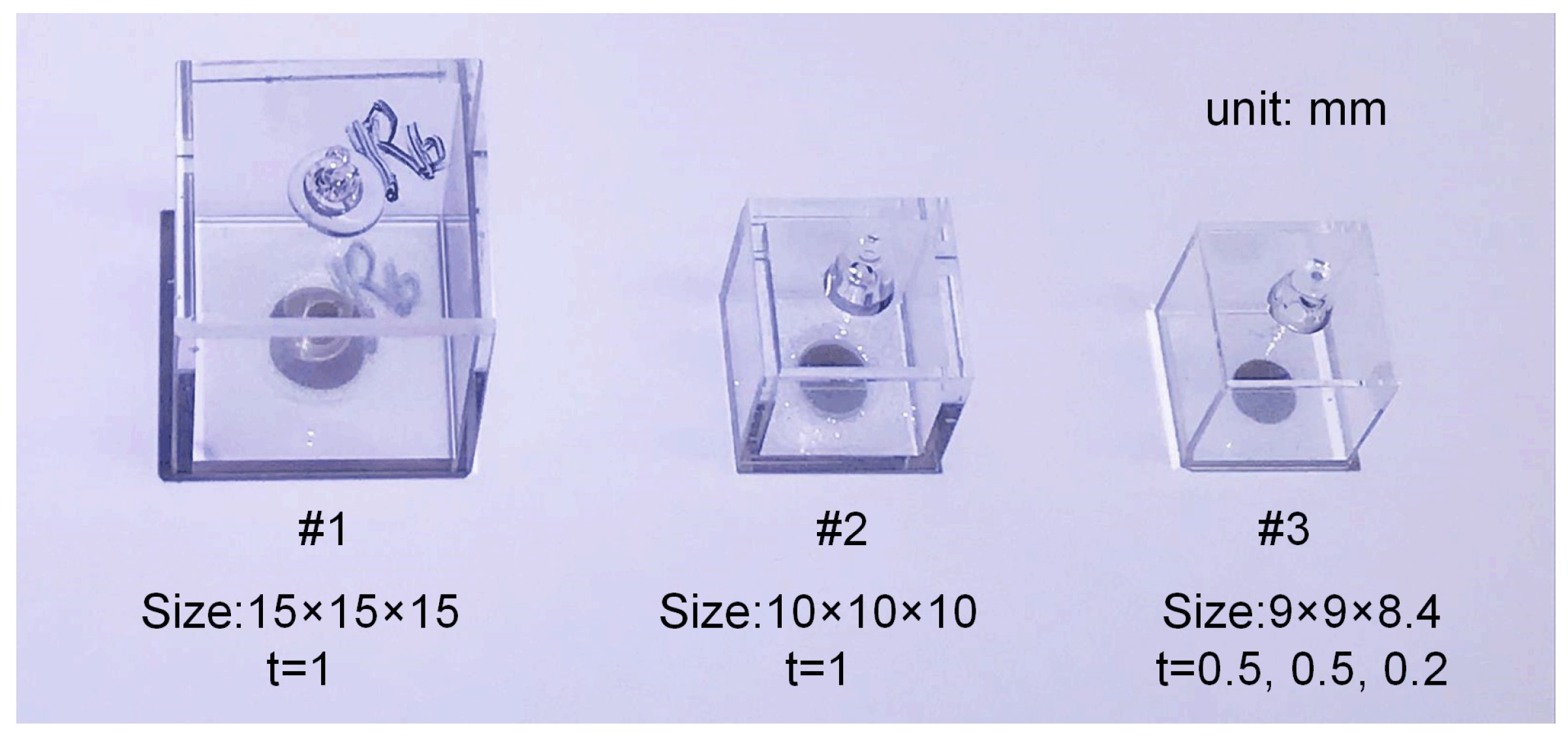
| Number | Dimensions (mm) | Resonant Frequencies (GHz) |
|---|---|---|
| 1 | 15 × 15 × 15, t 1 = 1 | 13.02, 14.87, 19.17, 20.01, 20.04 |
| 2 | 10 × 10 × 10, t = 1 | 18.01, 19.77, 24.68, 25.65, 26.44 |
| 3 | 8.4 × 8.4 × 8.4, t = 0.2 | 24.72, 29.67, 38.88, 39.03, 41.79 |
© 2018 by the authors. Licensee MDPI, Basel, Switzerland. This article is an open access article distributed under the terms and conditions of the Creative Commons Attribution (CC BY) license (http://creativecommons.org/licenses/by/4.0/).
Share and Cite
Song, Z.; Zhang, W.; Wu, Q.; Mu, H.; Liu, X.; Zhang, L.; Qu, J. Field Distortion and Optimization of a Vapor Cell in Rydberg Atom-Based Radio-Frequency Electric Field Measurement. Sensors 2018, 18, 3205. https://doi.org/10.3390/s18103205
Song Z, Zhang W, Wu Q, Mu H, Liu X, Zhang L, Qu J. Field Distortion and Optimization of a Vapor Cell in Rydberg Atom-Based Radio-Frequency Electric Field Measurement. Sensors. 2018; 18(10):3205. https://doi.org/10.3390/s18103205
Chicago/Turabian StyleSong, Zhenfei, Wanfeng Zhang, Qi Wu, Huihui Mu, Xiaochi Liu, Linjie Zhang, and Jifeng Qu. 2018. "Field Distortion and Optimization of a Vapor Cell in Rydberg Atom-Based Radio-Frequency Electric Field Measurement" Sensors 18, no. 10: 3205. https://doi.org/10.3390/s18103205