Odor Fingerprint Analysis Using Feature Mining Method Based on Olfactory Sensory Evaluation
by
 , ,
, ,
Hong Men
1,*, 
Yanan Jiao
1,
Yan Shi
1,
Furong Gong
1,
Yizhou Chen
2,
Hairui Fang
1 and
Jingjing Liu
1,*
1
Advanced Sensor Technology Institute, College of Automation Engineering, Northeast Electric Power University, Jilin 132012, China
2
Department of Neurobiology and Behavior, University of California, Irvine, CA 92697, USA
*
Authors to whom correspondence should be addressed.
Sensors 2018, 18(10), 3387; https://doi.org/10.3390/s18103387
Submission received: 15 September 2018
/
Revised: 6 October 2018
/
Accepted: 8 October 2018
/
Published: 10 October 2018
(This article belongs to the Special Issue Electronic Noses and Their Application)
Abstract
:In this paper, we aim to use odor fingerprint analysis to identify and detect various odors. We obtained the olfactory sensory evaluation of eight different brands of Chinese liquor by a lab-developed intelligent nose. From the respective combination of the time domain and frequency domain, we extract features to reflect the samples comprehensively. However, the extracted feature combined time domain and frequency domain will bring redundant information that affects performance. Therefore, we proposed data by Principal Component Analysis (PCA) and Variable Importance Projection (VIP) to delete redundant information to construct a more precise odor fingerprint. Then, Random Forest (RF) and Probabilistic Neural Network (PNN) were built based on the above. Results showed that the VIP-based models achieved better classification performance than PCA-based models. In addition, the peak performance (92.5%) of the VIP-RF model had a higher classification rate than the VIP-PNN model (90%). In conclusion, odor fingerprint analysis using a feature mining method based on the olfactory sensory evaluation can be applied to monitor product quality in the actual process of industrialization.
1. Introduction
Due to its particularity and generality, fingerprint can provide the basis to distinguish between samples due to its uniqueness and reliability [1]. Odor fingerprint analysis is preferred to the use of intelligent instruments which are sensitive to the stimulation of odor to produce the relevant data of volatile feature components. Adoption of odor fingerprint analysis is widely used in the field of foods. For example, the maturity of fruits could be expressed by the odor intensity [2], the degree of freshness [3], and diseases [4,5] could be determined by odor fingerprint analysis. Thus, the use of odor as a biometrics recognition method is feasible [6].
Chinese liquors belong to the distilled liquor which is loved by people for its strong aromatic odor. As a traditional fermented beverage, the saccharifying ferment of Chinese liquor is daqu, xiaoqu, bran koji and yeast wine, which is produced with cereal grains as the main raw materials and is processed by distilling, saccharifying and fermenting [7]. The microconstituents of liquors are organic compounds which directly influence the flavor of liquor quality. These organic contents are 1% to 2% including acids, esters, alcohols, aldehydes, and so on. Depending on the different brewing techniques and raw materials, different liquors have significant differences in aromatic characters and odor fingerprint. Therefore, the case study of Chinese liquor is representative and typical.
Currently, there are multiple studies on liquors by traditional sensory evaluation and physical or chemical methods [8,9]. With the advantages of simple operation and immediate results, the sensory evaluation method is generally acknowledged and widely adopted. However, this method mainly depends on the reviewers’ subjective sense of smell and taste [10]. In addition, there is a great deal of time and cost to train qualified professionals. On the other hand, the physical or chemical method analyzes samples using infrared spectrometer, chromatographic analyzer, mass spectrometer and other instruments [11,12]. These methods are reliable to analyze constituents of samples. However, there are some shortcomings, such as time-consuming, costs. These methods cannot comprehensively evaluate sample and cannot meet the development of process of industrialization.
Along with the rapid development of artificial intelligence, intelligent nose, also known as artificial nose, intelligent olfaction system, as a new bionic detection instrument, could make up the deficiency of the traditional olfactory sensory evaluation [13]. Intelligent nose consists of three parts: sensor array, signal processing unit, and pattern recognition. These three parts can respectively simulate the acquisition of information by human olfactory receptor sensory neurons, the encoding of the olfactory nerve, and the processing of information by the human olfactory system [14]. Therefore, odor fingerprint information gathered by intelligent nose could evaluate samples comprehensively. Based on the human olfaction, each olfactory neuron can detect different odorant molecules. On the other hand, each odorant molecule is able to respond to multiple olfactory neurons. The same goes for the principle of intelligent nose: Different sensors respond differently to different odorants. The intelligent nose can provide overall information of volatile compounds and it is widely used in analyzing the quality of wine [15], tobacco [16], tea [17], rice [18] and fruit [19,20,21]. Furthermore, it also involved in medical diagnosis [22], environment monitoring [23] and other fields. However, there are only a handful of published studies focusing on the detection of odor fingerprint information of Chinese liquors using intelligent nose, such as analyzing different flavor types [24], authenticity [25], place origin [26] and age [27].
As is known to all, drift is an inevitable question in measurement. Sensor drift refers to the output of sensor changes from time to time when the input remains unchanged. Currently, it is believed that sensor drift is caused by two causes, on the one hand is the chemical process which occurs between the sensor material and the environment, on the other hand is the system noise [28]. In practice, the outputs gradually fail to match the right gases for sensor drift reason. For this problem, researchers have done a great deal of work to ensure the response of sensors. Ma et al. [28] proposed the ODAELM-S and ODAELM-T for online sensor drift compensation in E-Nose systems. This method aims to achieve timely processing without losing the recognition accuracies for sensor drift. Zhang et al. [29] proposed the DAELM-S and DAELM-T to compensate sensor drift. Another effective method is unsupervised feature adaptation (UFA)-based transfer, learning ideas for enhancing the drift tolerance of E-noses [30]. The above methods focus on online compensation to resolve the sensor drift effectively.
In this paper, taking Chinese liquors as an example, we followed the offline sensor drift compensation approach for the intelligent nose system while the majority of past studies have focused on the simulation of human olfaction to detect and identify odor fingerprint information.
The appropriate multivariate statistical and pattern recognition methods can effectively increase the differentiation of odor fingerprints based on the intelligent nose and can check the accuracy of models. Previous research primarily focused on the feature extraction of time domain features such as peak, mean, maximum variance, root mean square and standard deviation [31,32]. However, the basic characteristics of signals, both in the time domain and frequency domain, can provide comprehensive angles for signal analysis. The time domain is the only real domain which is parallel to the real world and it is the relationship between mathematical functions and physical signals to time. While the frequency domain is a mathematical category which follows particular rules which can reveal the inner characteristics signals [33,34]; the feature extraction method, combining time domain and frequency domain features, can be used to mine information that reflects different odor fingerprint features about samples [35,36]. However, this method causes information redundancy, that is, as the number of dimensions increases, the training time and forecasting time of the model will take longer. Therefore, it is of greatest importance to find a more reasonable and effective feature mining method to extract efficient features.
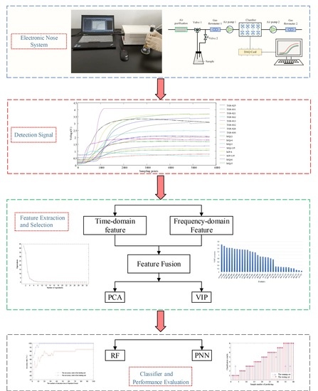
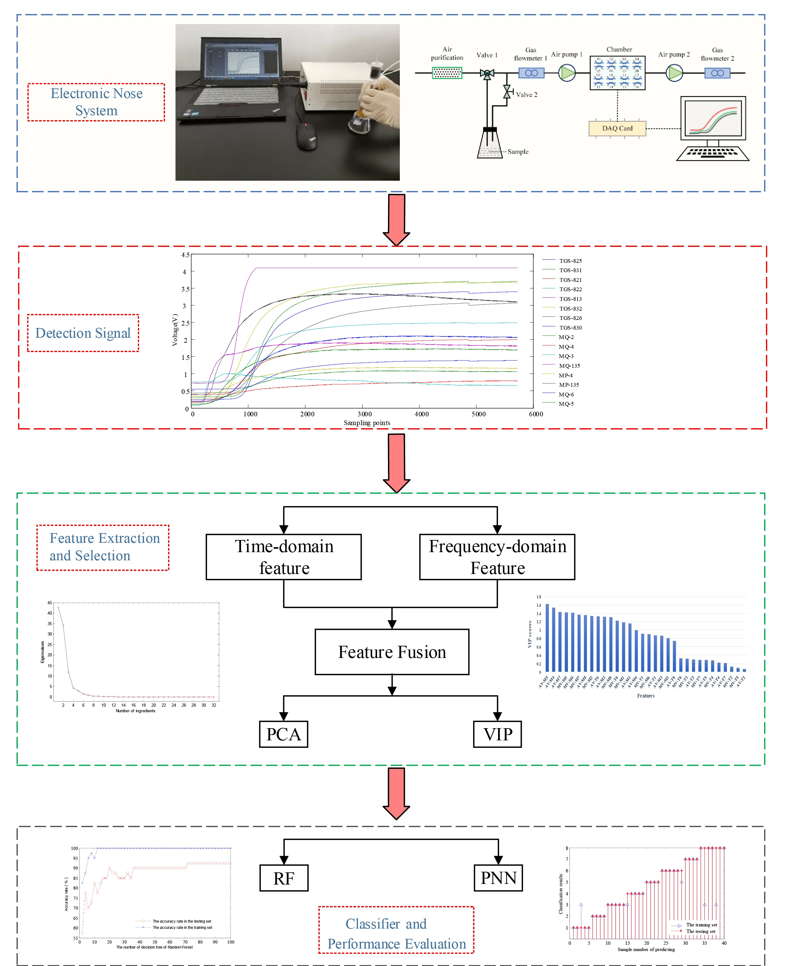
Taking eight different brands of Chinese liquors as an example, this paper aims to use the odor fingerprint analysis, simulate human olfaction through experiments with the lab-developed intelligent nose and adopt the feature mining method to detect and identify various odors. According to the raw experimental data from 16 sensors of the lab-developed intelligent nose, we extracted the time domain and frequency domain characteristics to construct the odor fingerprint. In addition, odor fingerprints were analyzed by PCA and VIP scores for selecting characteristic features. Next, we selected Random Forest (RF) and Probabilistic Neural Network (PNN) to dynamically characterize the interactions among the feature variables, and then obtained the best variable characteristics and the highest classification accuracy. This is a significant study for the detection and identification of Chinese liquors through odor fingerprint analysis based on the olfactory sensory evaluation. Figure 1 shows the flow chart of odor fingerprint analysis for this article.
2. Materials and Methods
2.1. Liquor Samples
In this paper, eight different brands of Chinese liquors purchased at a local liquor store were selected as samples. These samples differed in brand, alcohol content, flavor, raw materials, and origin. Details were listed in Table 1.
2.2. Intelligent Nose
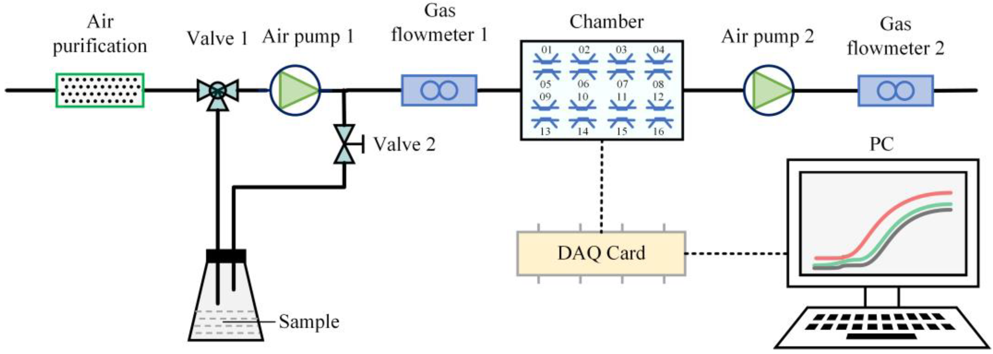
As shown in Figure 2, the lab-developed intelligent nose system contains three units—the air flow velocity and direction control unit (consists of air purification, valve, gas flowmeter, and air pump), the sensors unit (includes sensor arrays and chamber), and the data acquisition and analysis unit (contains data acquisition card (DAQ) and PC with the self-made test software). The two major functions (gas injection and system cleaning) were carried out by adjusting valves. The air purification consists of activated carbon, molecular sieve and allochroic silicagel gel, and more remarkably, allochroic silicagel gel, which belongs to the high-grade drying agent, can visually signal the relative humidity of the environment according to the color variation (from blue to red). It is usually used for instruments, equipments and other closed conditions. The role of air pump 1 and 2 are to clean the system and to collect gas, respectively. In addition, the combination of these two air pumps are used to raise the gas volume rate in the gas cleaning process. The dimension of the chamber is 10.5 cm long, 8.2 cm wide and 5 cm high with a volume of about 431 cm3. The chamber is made of cardboard which is covered by Polytetrafluoroethylene (PTFE). PTFE has weak adsorption and strong leakproofness so that there is no other interfering research to affect the test results in the air chamber. Sensor arrays contain a temperature sensor, humidity sensor and 16 independent sensors. LM35CZ type temperature sensor by National Semiconductor, Santa Clara, CA, USA and HIH-4000-003 type humidity sensor by Yi Jiajie Electronic Technology CO., LTD, ShenZhen, China, in the air chamber are used to monitor the internal temperature and humidity. Sixteen independent sensors are sensitive to different substances. These sensors can detect odor fingerprint data and consist of two systems: TGS-8 system by FIGARO, Japan and MQ/MP system by ZhengZhou Winsen Electronics Techbology CO., LTD, ZhengZhou, China. Details of these sensors used in the experiment are listed in Table 2. The NI USB-6211 type data acquisition card by National Instruments, Austin, TX, USA, was selected to collect data. There are eight analog input channels and two analog output channels and the sample rate reaches 48 Ks/s.
The static head-space sampling method was adopted in this experiment. The lab environment is best to control the temperature at 23 ± 2 °C and the relative humidity at 60 ± 5%. The experimental procedure was performed as following:
(1) Open the air pump 2 and valve 1, put a clean and empty Erlenmeyer flask in the defined location. Then observe the zero value of each sensor and compare with the standard value.
(2) Twenty milliliters of the sample was put in a 100 mL Erlenmeyer flask, sealed and left to sit for 5 min.
(3) Close air pump 2 and adjust air pump 1 so that the gas flowmeters 1 and 2 (by Qihai Electromechanical Manufacturing CO., LTD, Chengdu, China) display 2 L/min to clean windpipes for 10 s. Then open air pump 2 to clean the entire device. This process lasted 5 min to eliminate the influence by other gases.
(4) Place the test samples in the defined location and adjust air pumps 1 and 2 so that the gas flowmeters 1 and 2 display 0.5 L/min to let the gas enters the chamber. Ten seconds later, close air pump 2 and keep the gas coming into the chamber sequentially. At the same time, observe the signals and record test data.
(5) Without loss of generality, repeat the experiment 10 times for each sample by repeating Steps (2)–(4). Note that the relative humidity will not change in the course of the experiment. At last, a total of 80 sets of data is obtained.
In this paper, we extracted time domain and frequency domain features to construct an odor fingerprint map. The time-domain feature is the average value (AV) of intelligent nose response signals of sensors. The frequency domain feature is the mean of variance (MV) of the eight wavelet packet coefficients obtained by three layers of wavelet packet decomposition with db6 wavelet [37].
The time domain features of the ith sensor of TGS-8 system were defined as:
where xTi1, xTi2, …, xTi5940 are response value of the ith sensor of TGS-8 system intelligent nose.
The time domain features of the ith sensor of the MQ/MP system were defined as:
where xMi1, xMi2, …, and xMi5940 are response values of the ith sensor of the MQ/MP system electronic nose.
The time domain features of the ith sensor of the TGS-8 system were defined as:
where STi1, STi2, …, STi8 are the variance yields extracted from the coefficients of the wavelet packet of the ith sensor of the TGS intelligent nose; the response value measured from the intelligent nose was decomposed into wavelet packet components based on the db6 wavelet, and then extracting the coefficients of the wavelet packet.
The frequency domain features of the ith sensor of the MQ/MP system were defined as:
where SMi1, SMi2, …, SMi8 in the formula are the variance yields extracted from coefficients of wavelet packet of the ith sensor of the MQ/MP intelligent nose; the response value measured from the intelligent nose was decomposed into wavelet packet components based on the db6 wavelet, and then extracting the coefficients of the wavelet packet.
2.3. Feature Selection
2.3.1. Data Processing of Odor Fingerprint Analysis
As is known to all, sensor sensitivity has a great influence on the intelligent nose system performance. The sensitivity of the sensor should be considered to achieve the best performance.
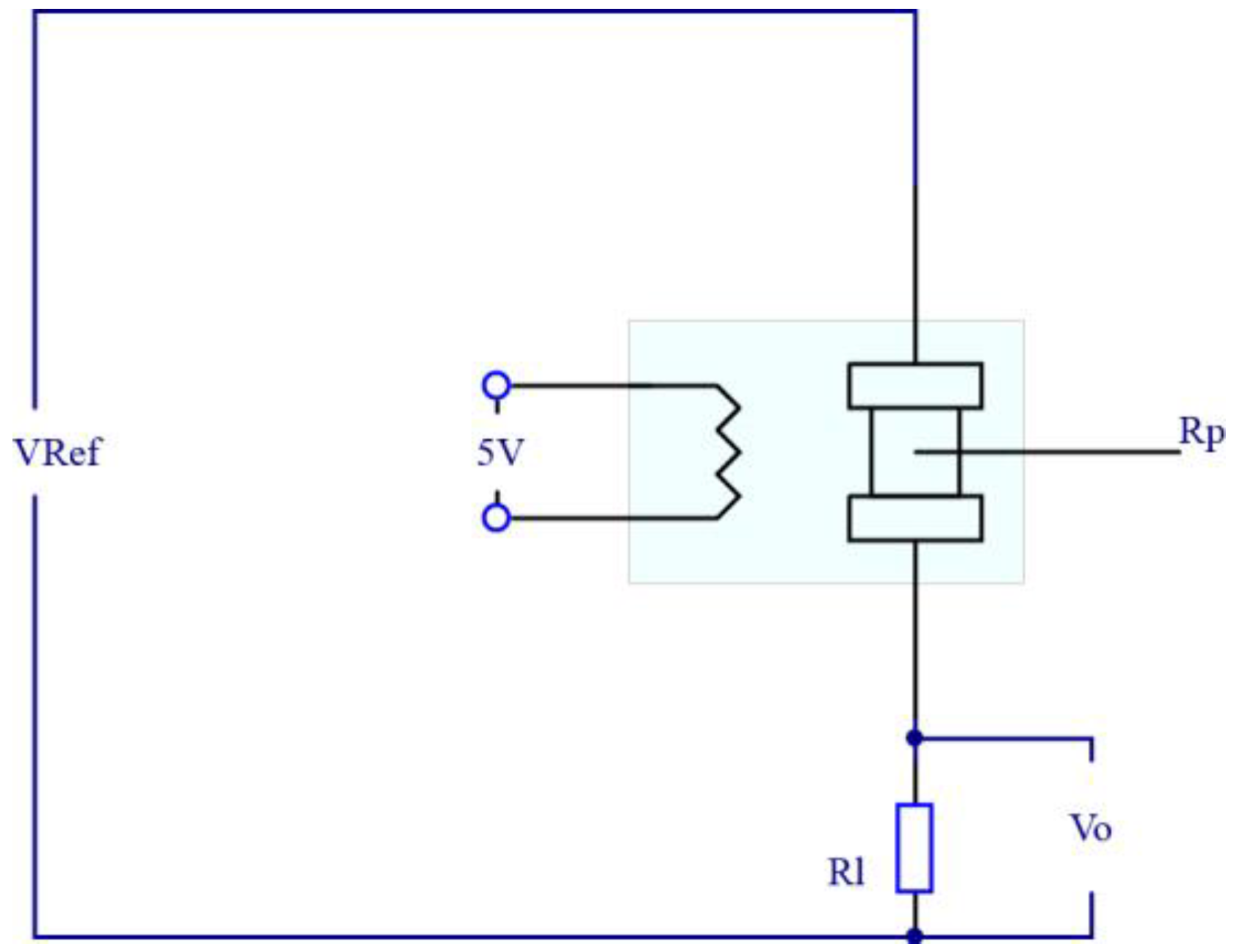
As shown in Figure 3, in the drive circuit of the sensor, Rp is the resistance value of the sensor. Rl is the resistance value of the load resistance and the output voltage of sensor is the voltage across the load resistance. The relationship between the output voltage and reference voltage is as follows:
All these show that when Rl is equal to Rp, the sensor has the greatest response sensitivity to improve the performance of the intelligent nose system.
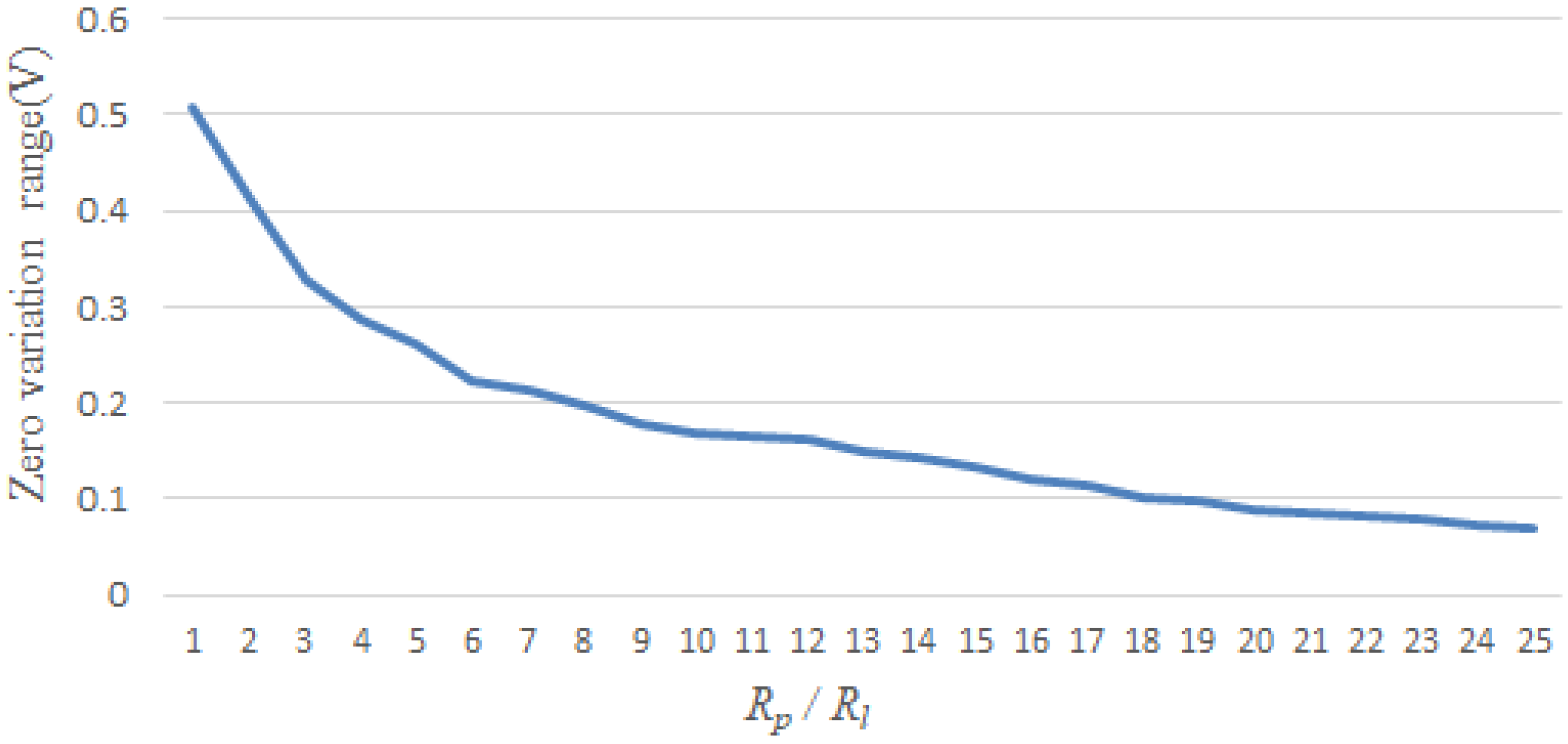
As shown in Figure 4, taking the TGS-821 sensor for example, the best output response was studied by changing different Rl values. Other sensors have the same characteristics.
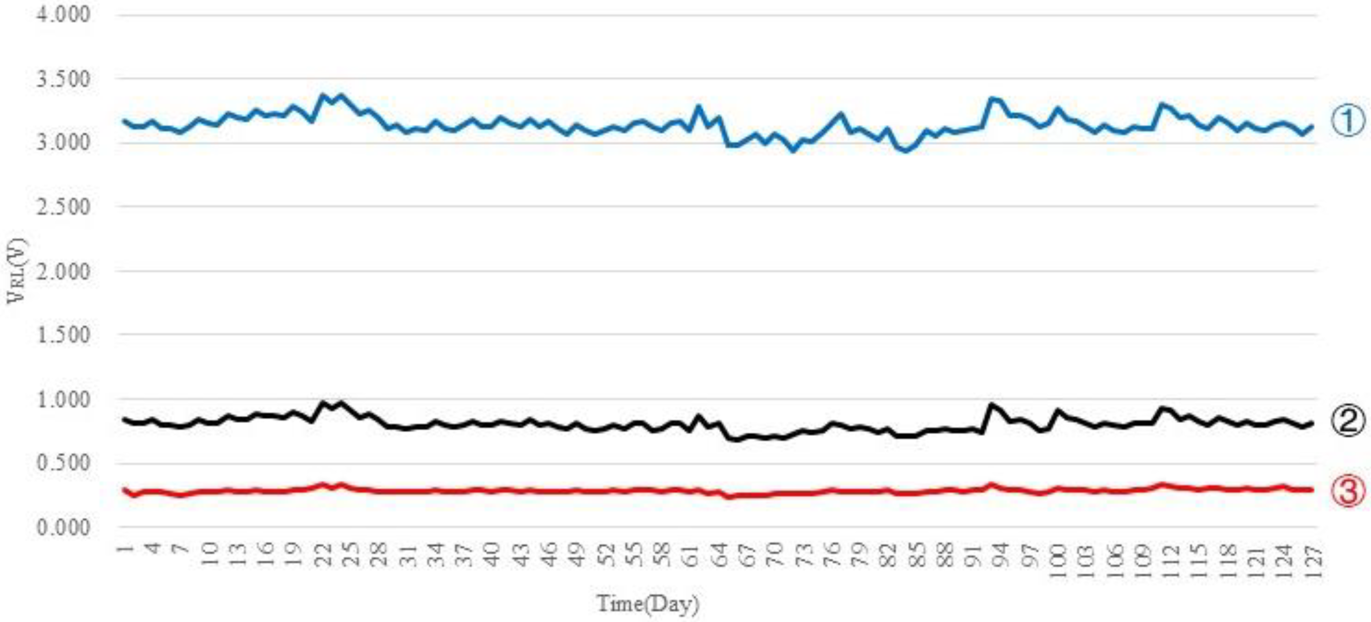
As shown in Figure 5, in order to find the appropriate resistance value of the load resistor in experiment, we perform an experiment with the purpose of supervising the zero value of sensors which continued for 127 days. By experiment, when Rl is about one-fifteenth of the value of Rp, the output response of sensors is obvious.
Signal processing, as an important step of improving the performance of the intelligent nose, refers to preprocess signals of sensor array responses. The standardized processing is the most popular method that translates raw data into a dimensionless index. Therefore, this step can avoid pattern recognition failure because of the large magnitude of some sensors. We choose the relative difference method to suppress sensor drift. xs(0) is the zero response value of the sensor.
Then, in order to expedite the convergence rate of the model, the odor fingerprint information obtained by different sensors should be converted to the same dimension and the same order of magnitudes. We normalized the fusion feature sets and the normalized interval is (0, +1). After the series of the above-mentioned processing (relative difference method and normalization), additive drift and response drift of the sensor will be suppressed.
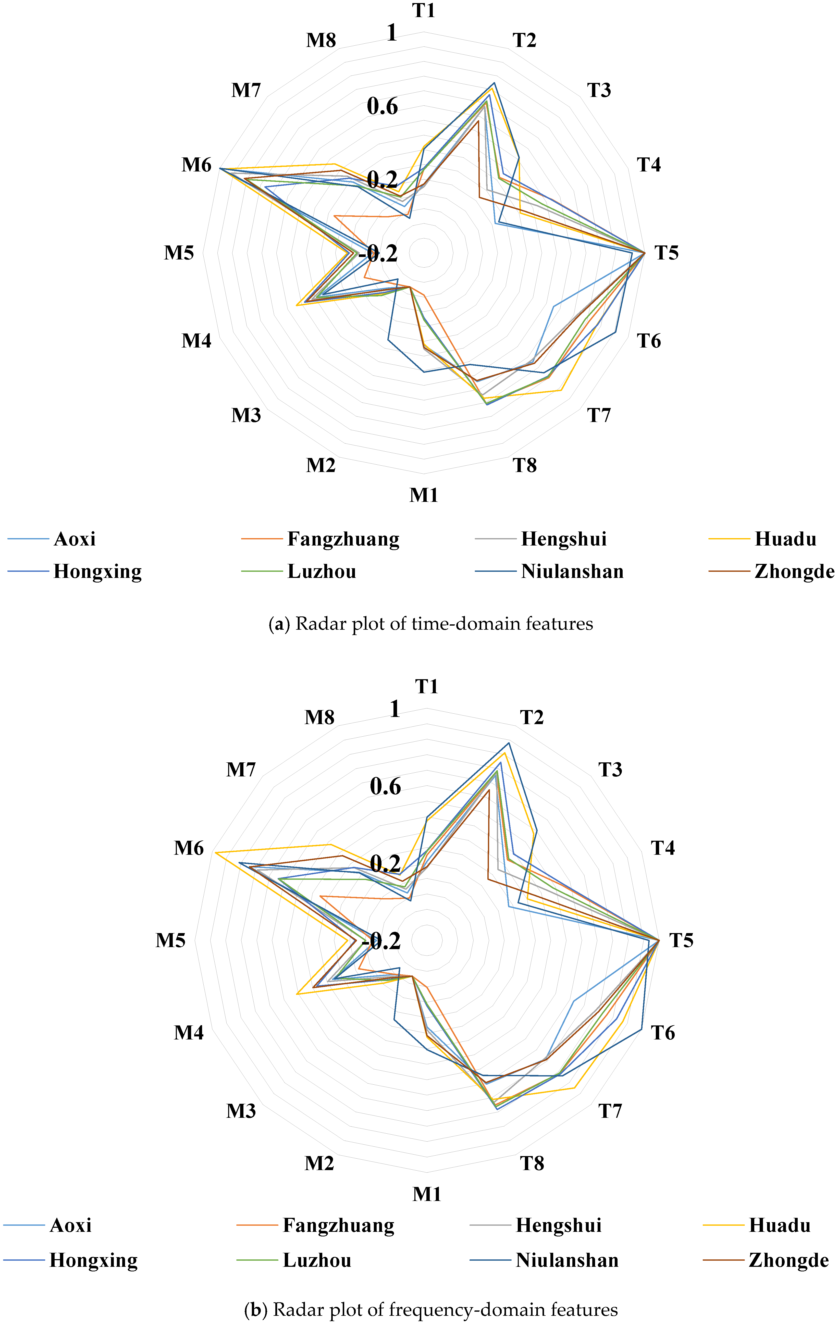
Figure 6a,b shows radar plots for time domain and frequency domain features, respectively. Since each sensor detects cross-information of olfactory, it is difficult to determine which features are the characteristic values that affect the olfactory information of liquors. It can be seen that the sensor T3 and T4 are obviously different in AV value. Does it proves these two values are the main factors affecting the olfactory information of Chinese liquors? Meanwhile, the sensor M1 and M2 are slightly difference in MV value. Does it proves these two characteristics have little effect on the olfactory information of Chinese liquors? Therefore, it is indispensable to find a suitable feature mining method to delete the redundant information and select characteristic features that can affect the olfactory information of Chinese liquors. In addition, the best combination of variables and fusion methods to reduce the complexity of the model prediction and achieve the best classification performance have to be chosen.
2.3.2. Feature Extraction and Filtering
Principal Component Analysis (PCA) is a meaningful multivariate statistical method. It can convert multiple variables to a few comprehensive variables through linear transforming. These comprehensive variables that are principal components can reflect most of the information of the original variables at the greatest extent. These principal components are not only linearly independent of each other but also mutually orthogonal. In this paper, PCA was used to process the original features that fused the time domain and frequency domain. From this, principal components can express characteristic features of Chinese liquors’ olfactory information.
In the Partial Least Square (PLS), the Variable Importance of Projection (VIP) scores were used to create a new data space in a lower dimensional system [38]. The VIP scores can express the interpretative ability of the independent variables to dependent variables. With higher scores meaning a greater rate of contribution to covariance and stronger distinguishing ability, each variable of the original feature was evaluated and obtained corresponding scores. These variables were sorted based on the VIP scores and selected to form the new characteristic space. The feature fusion strategy is as follows: (1) The original features that fused time domain and frequency domain were sorted based on VIP scores. (2) K = [k1, k2, …, km] variable subsets were generated based on the best VIP scores. Which ki means the subset has top ith variables and m is the number of all variables. In this paper, we analyzed the original features and generated 32 subsets based on the VIP scores to express the interaction between different variables.
2.3.3. Multivariate Analysis
In this paper, altogether 80 sets of data were divided into two parts based on the Kennard-stone algorithm, 1/2 as the training set and the rest as the testing set. The former was used to construct the classification model and the latter was used to test the classification performance of models established by the former.
The KS algorithm is commonly used as an effective method to select a training set. In the KS algorithm, all samples were considered as candidates for training sets that were selected in order. The KS algorithm can be summarized as follows: (1) Calculating the distance between every two samples and selecting the two samples with the largest distance. (2) Calculating the distance between the remaining sample and the selected two samples, respectively. (3) Repeating this step until the number of selected samples is equal to the predetermined number [39].
Random Forest (RF) is an ensemble of classification and regression tree (CART). It was first proposed by Kam in 1995 [40] and Breiman made an intensive study [41]. The essence of RF is a nonlinear classifier that contains multiple decision trees. There is no correlation between these trees. When the testing data entered into the random forest, the data was classified by each decision tree. The final results are the most classified results in all trees.
With its fast training rate and simple realization, it is widely used in biological information [42], ecology [43], medicine [44], economic finance [45], computer vision [46], speech [47], data mining [48], remote sensing geography [49] and other fields. The execution procedure of RF is: Assuming that the number of attributes of the sample is M. Resampling based on the Bootstrap method. Then T training sets S1, S2, …, ST were generated. (2) The corresponding decision trees C1, C2, …, CT were generated by each training set. Before the property was selected on each internal node, m properties that were randomly selected from M properties should be seen as the split attribute set of the current node. (3) Each tree has complete growth without pruning. (4) For the testing set sample X, every decision tree was tested to obtain the corresponding categories C1(X), C2(X), …, CT(X). (5) By taking the vote, the most output category in the T decision trees was taken as the category of the testing set.
Probabilistic Neural Networks (PNN) is the supervised classifier which was first put forward by D. F. Speeht in 1990 [50]. It is a parallel algorithm based on the Bayes classification rule and the Parzen window’s probability density function. With its simple learning process, fast training speed, better compatibility and strong nonlinear ability, PNN was applied to image recognition [51], chemical detection [52] and stereo vision matching [53] fields. PNN generally consists of four layers: The input layer, the model layer, the summation layer, and the output layer. The steps of PNN networks are as follows: (1) Collecting sample data and dividing into a training set and a testing set. (2) Creating PNN networks and training the network according to training sets. (3) Testing network performance.
3. Results
3.1. Dimension Reduction by PCA
The odor fingerprint information obtained in the experiment was analyzed by the PCA algorithm. The first three principal components account for 42.59%, 34.16%, and 11.95% respectively. Figure 7a shows the PCA processing results of different brands of Chinese liquors.
Observing the scree plot from Figure 7b, when the number of principal components reaches 10, the polyline area is stable. The cumulative contribution of principal components reaches 99.368%, which can represent all characteristic data. Therefore, we extracted the first 10 principal components as a new feature data set to substitute the original variables. Results showed that it provides a reliable method to construct a little more concise odor fingerprint map.
3.2. Variable Selection by VIP Scores
Figure 8 shows the VIP scores for each feature variable of the original fusion dataset measured by PLS discrimination analysis. As shown, the VIP score of AVM5, AVM4, AVM7, MVM5, MVM4, MVM7, AVM8, MVM2, AVT6, AVM2, MVM8, MVT6, MVM1 and AVM1 are greater than 1, indicating that these variables have significant meaning in the odor fingerprint of Chinese liquors. While the VIP scores of the rest are less than 1, which means that these variables have less effect on the classification of Chinese liquors, VIP scores cannot give a verdict for the classification performance of models. Therefore, we found a series of fusion matrix as an input of the model based on VIP scores. Each subset includes the top several variables, in other words, subset #1 includes AVM5, subset #2 contains AVM5 and AVM4, the last subset #32 contains all variables. We can select the prime variable combination by dynamically observing the classification performance of RF networks and PNN network. Results showed that it provides a reliable method to construct a much more concise odor fingerprint map by selecting the best combination of variables.
Table 3 shows the accuracy rate achieved by RF and PNN models. As the number of variables increases, the classification accuracy rates show an upward tendency. Specifically, the classification accuracy of RF and PNN in subset #11 have reached the same accuracy as the original fusion dataset. This indicates that the original fusion dataset contains a large amount of redundant information. With the number of variables increasing, RF models appeared to have the highest accuracy rate of 92.5% under the subset #15 and PNN appeared to have the highest accuracy rate of 87.5% under subset #16. We continued to raise variables, and the accuracy rate of each model did not exceed the above-mentioned maximum value. These results are consistent with the VIP scores shown in Figure 8. That is, the performance of the model increased with variables added whose VIP scores were greater than one, while the performance of the model decreased with the rest of the variables added whose VIP scores were less than one. From above, we chose subset #15 as the best combination.
3.3. Classification Using Random Forest
In RF networks, the value of mtry and the number of decision trees are the main parameters of generalization performance. The default mtry value is the square root of the total number of variables, so the value of mtry in the experiment was four. We selected the number of decision trees from 2 to 100 at two trees intervals. The training accuracy rate and predicting accuracy rate were regarded as the evaluation criterion. From this, we can focus on the influence of decision trees on the classification performance in RF networks.
The three feature sets (original, PCA-optimized, and VIP-optimized, from which the 15th variable subset was extracted based on the VIP scores) combined with the RF model achieved the classification for olfactory information of Chinese liquors. To reduce the impact of randomness, 100 prediction models were established, and their accuracy rates were averaged as the classification accuracy rate of the current model. As shown form Figure 9a–c, the training accuracy rate reaches 100% when the number of decision trees is greater than 8, 4, and 12, respectively. Besides, in the RF model based on the VIP-optimized feature set, when the number of decision trees exceeds 72, the testing accuracy reaches up to 92.5%. Further, along with the continual increase of the decision trees, the system remains stable. Results showed that the olfactory information of original features contains redundant information. Besides, the feature mining method based on VIP-optimized can extract effective features.
3.4. Classification Using PNN
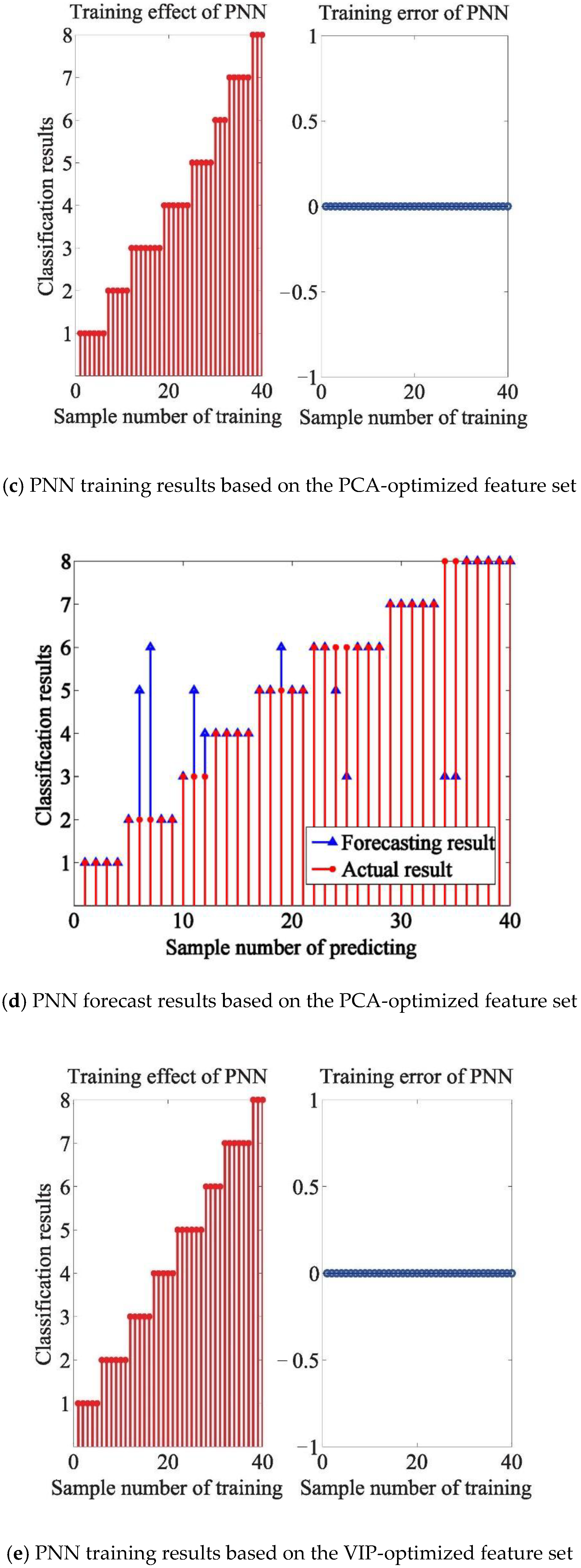
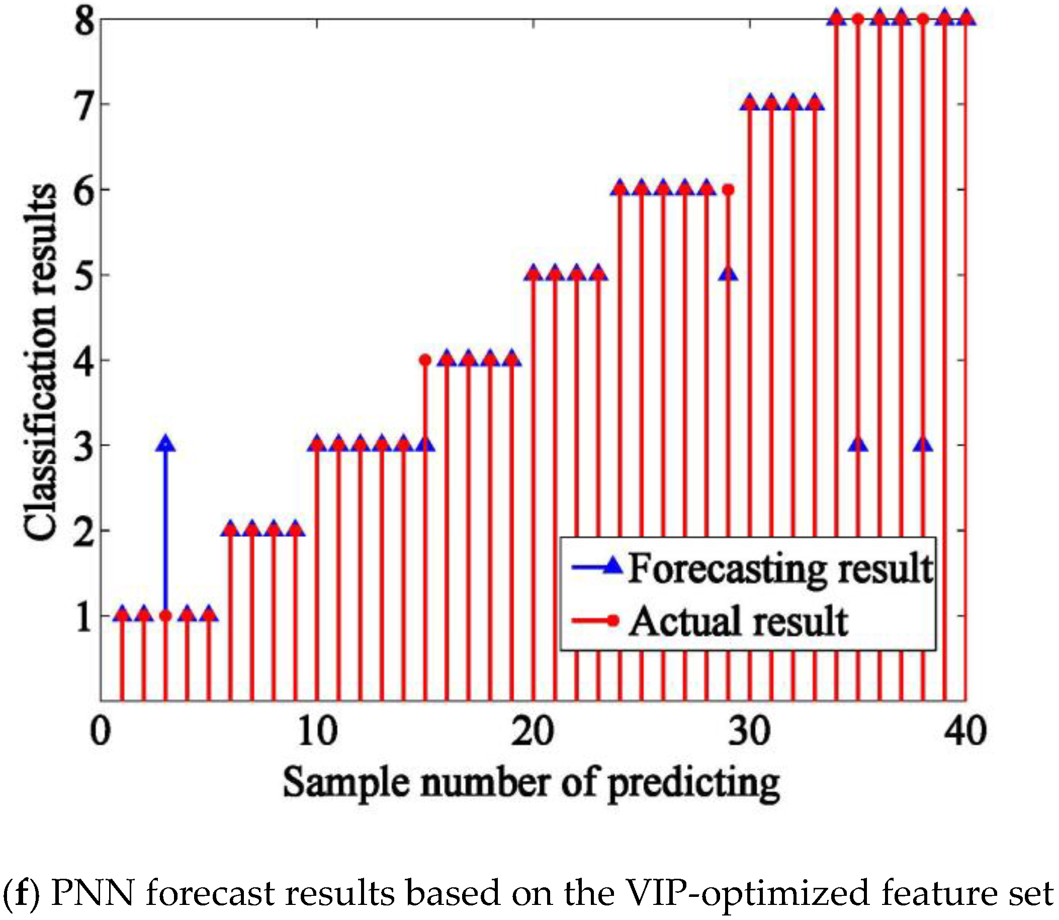
The three feature sets (original, PCA-optimized, and VIP-optimized from which the 16th variable subset was extracted based on the VIP scores) combined with the PNN model work well in classifying the olfactory information of Chinese liquors. As shown in Figure 10a,c and e, 40 training samples were classified correctly, as shown in predicting effect of PNN, the test accuracy rate was 65%, 77.5% and 87.5% with 40 test samples (The vertical axis is category label. And from 1 to 8 are category labels of eight brands of Chinese liquors, respectively.).
The PNN models based on PCA-optimized and VIP-optimized are superior to the model based on the original features, which means that there is a lot of redundant information in the original features. Compared with the PNN model based on PCA-optimized, the model of VIP-optimized performed well, which means that the feature mining method based on VIP-optimized can improve the accuracy rate and extract effective features.
4. Discussion
Table 4 shows the classification accuracies under different data processing and pattern recognition methods. As shown in Table 4:
(1) By comparison, the classification accuracy of the RF network was better than the PNN network based on the different feature methods. Thus, it can be seen that the RF network has stronger processing power in this experiment.
(2) Compared with the original features, classification performance did not significantly improve based on the PCA-optimized both in the RF network and PNN network. The data processing method based on PCA cannot obtain the best combination of variables to identify various odors more accurately.
(3) Compared with the original feature and PCA-optimized, selected features based on the best VIP scores obtained the obvious promotion of the classification performance. The classification accuracy of the RF network in subset #15 and the PNN network in subset #16 was 92.5% and 87.5%, respectively. Finally, the RF network showed the best classification performance of 92.5% in subset #15. Combined with VIP scores, AVM5, AVM4, AVM7, MVM5, MVM4, MVM7, AVM8, MVM2, AVT6, AVM2, MVM8, MVT6, MVM1, AVM1, and AVM6 were considered as the characteristic features.
5. Conclusions
In conclusion, taking eight different brands of Chinese liquors as an example, our work adopted the odor fingerprint analysis based on olfactory sensory evaluation and the feature mining method which combined the time domain and frequency domain to simulate human olfaction and to identify various odors. Variable selection using VIP scores is especially suitable for extracting features from a mass of data. In addition, the VIP-based models achieved better prediction accuracies than the PCA’s. The results demonstrated that VIP coupled with the RF or PNN network is effective in extracting and analyzing features of odor fingerprint. Compared with the PNN model, the RF model achieved the slightly higher accuracy. Meanwhile, compared with the traditional statistical methods and simple extraction, this feature mining method used the least characteristic variables and the best fusion method and can capture hidden patterns and variables inside the odor fingerprint. The odor fingerprint analysis using the feature mining method based on olfactory sensory evaluation can be applied to the food and drinks industry for product discrimination, classification, quality and control. Besides, the lab-developed intelligent nose can be used in the actual process of industrialization to monitor product quality.
Author Contributions
H.M. and J.L. conceived and designed experiments. Y.J. analyzed the data and wrote the paper. Y.S. and F.G. performed the experiment to obtain the olfactory information. Y.C. and H.F. extracted the olfactory characteristic information.
Funding
This paper supported by the National Natural Science Foundation of China (31772059, 31871882), the Provincial Special Funds for Industrial Innovation of Jilin Province (2018C034-8), the Key Science and Technology Project of Jilin Province (20170204004SF) and the Graduate Innovation Fund Project of Northeast Electric Power University (Y2017014).
Conflicts of Interest
The authors declare no conflict of interest.
References
- Baldisserra, D.; Franco, A.; Maio, D.; Maltoni, D. Fake Fingerprint Detection by Odor Analysis International Conference on Advances in Biometrics. In Proceedings of the International Conference on Biometrics, Hong Kong, China, 5–7 January 2006; pp. 265–272. [Google Scholar]
- Kinjo, H.; Oshiro, N.; Duong, S.C. Fruit maturity detection using neural network and an odor sensor: Toward a quick detection. In Proceedings of the 10th Asian Control Conference, Kota Kinabalu, Malaysia, 31 May–3 June 2015; pp. 1–4. [Google Scholar]
- Lee, K.M.; Son, M.; Kang, J.H.; Kim, D.; Hong, S.; Park, T.H.; Chun, H.S.; Choi, S.S. A triangle study of human, instrument and bioelectronic nose for non-destructive sensing of seafood freshness. Sci. Rep. 2018, 8, 547. [Google Scholar] [CrossRef] [PubMed]
- Covington, J.A.; Wedlake, L.; Andreyev, J.; Ouaret, N.; Thomas, M.G.; Nwokolo, C.U.; Bardhan, K.D.; Arasaradnam, R.P. The detection of patients at risk of gastrointestinal toxicity during pelvic radiotherapy by electronic nose and FAIMS: A pilot study. Sensors 2012, 12, 13002–13018. [Google Scholar] [CrossRef] [PubMed]
- Dymerski, T.; Gębicki, J.; Wiśniewska, P.; Śliwińska, M.; Wardencki, W.; Namieśnik, J. Application of the Electronic Nose Technique to Differentiation between Model Mixtures with COPD Markers. Sensors 2013, 13, 5008–5027. [Google Scholar] [CrossRef] [PubMed] [Green Version]
- Gibbs, M.D. Biometrics: Body odor authentication perception and acceptance. ACM SIGCAS Comput. Soc. 2010, 40, 16–24. [Google Scholar] [CrossRef]
- Huo, D.Q.; Yin, M.M.; Hou, C.J.; Hui, Q.; Zhang, M.M.; Dong, J.L.; Luo, X.G.; Shen, C.H.; Zhang, S.Y. Identification of Different Aromatic Chinese Liquors by Colorimetric Array Sensor Technology. Fenxi Huaxue 2011, 39, 516–520. [Google Scholar]
- Rochaparra, D.; Chirife, J.; Zamora, C.; De Pascual-Teresa, S. Chemical Characterization of an Encapsulated Red Wine Powder and Its Effects on Neuronal Cells. Molecules 2018, 23, 842. [Google Scholar] [CrossRef] [PubMed]
- Gonzalez Viejo, C.; Fuentes, S.; Torrico, D.; Howell, K.; Dunshea, F.R. Assessment of beer quality based on foamability and chemical composition using computer vision algorithms, near infrared spectroscopy and machine learning algorithms. J. Sci. Food Agric. 2018, 98, 618–627. [Google Scholar] [CrossRef] [PubMed]
- Chira, K.; Teissedre, P.L. Chemical and sensory evaluation of wine matured in oak barrel: Effect of oak species involved and toasting process. Eur. Food Res. Technol. 2015, 240, 533–547. [Google Scholar] [CrossRef]
- Plutowska, B.; Wardencki, W. Application of gas chromatography-olfactometry (GC-O) in analysis and quality assessment of alcoholic beverages—A review. Food Chem. 2008, 107, 449–463. [Google Scholar] [CrossRef]
- Di, S.V.; Avellone, G.; Bongiorno, D.; Cunsolo, V.; Muccilli, V.; Sforza, S.; Dossena, A.; Drahos, L.; Vekey, K. Applications of liquid chromatography-mass spectrometry for food analysis. J. Chromatogr. A 2012, 1259, 74–85. [Google Scholar]
- Winquist, F.; Lundström, I.; Wide, P. The combination of an electronic tongue and an electronic nose. Sens. Actuators B Chem. 1999, 58, 512–517. [Google Scholar] [CrossRef]
- Persaud, K.; Dodd, G. Analysis of discrimination mechanisms in the mammalian olfactory system using a model nose. Nature 1982, 299, 352–355. [Google Scholar] [CrossRef] [PubMed]
- Buratti, S.; Benedetti, S.; Scampicchio, M.; Pangerod, E.C. Characterization and classification of Italian Barbera wines by using an electronic nose and an amperometric electronic tongue. Anal. Chim. Acta 2004, 525, 133–139. [Google Scholar] [CrossRef]
- Luo, D.; Hosseini, H.G.; Stewart, J.R. Application of ANN with extracted parameters from an electronic nose in cigarette brand identification. Sens. Actuators B Chem. 2004, 99, 253–257. [Google Scholar] [CrossRef]
- Bhattacharyya, N.; Seth, S.; Tudu, B.; Tamuly, P.; Jana, A.; Ghosh, D.; Bandyopadhyay, R.; Bhuyan, M. Monitoring of black tea fermentation process using electronic nose. J. Food Eng. 2007, 80, 1146–1156. [Google Scholar] [CrossRef]
- Lu, L.; Deng, S.; Zhu, Z.; Tian, S. Classification of Rice by Combining Electronic Tongue and Nose. Food Anal. Methods 2015, 8, 1893–1902. [Google Scholar] [CrossRef]
- Xu, S.; Lü, E.; Lu, H.; Zhou, Z.; Wang, Y.; Yang, J.; Wang, Y. Quality Detection of Litchi Stored in Different Environments Using an Electronic Nose. Sensors 2016, 16, 852. [Google Scholar] [CrossRef] [PubMed]
- Baietto, M.; Wilson, A.D. Electronic-Nose Applications for Fruit Identification, Ripeness and Quality Grading. Sensors 2015, 15, 899–931. [Google Scholar] [CrossRef] [PubMed] [Green Version]
- Brezmes, J.; Llobet, E.; Vilanova, X.; Orts, J.; Saiz, G.; Correig, X. Correlation between electronic nose signals and fruit quality indicators on shelf-life measurements with pinklady apples. Sens. Actuators B Chem. 2001, 80, 41–50. [Google Scholar] [CrossRef]
- Wang, P.; Tan, Y.; Xie, H.; Shen, F. A novel method for diabetes diagnosis based on electronic nose. Biosens. Bioelectron. 1997, 12, 1031–1036. [Google Scholar] [PubMed]
- Nicolas, J.; Romain, A.C.; Ledent, C. The electronic nose as a warning device of the odour emergence in a compost hall. Sens. Actuators B 2006, 116, 95–99. [Google Scholar] [CrossRef] [Green Version]
- Zhang, Q.; Xie, C.; Zhang, S.; Wang, A.; Zhu, B.; Wang, L.; Yang, Z. Identification and pattern recognition analysis of Chinese liquors by doped nano ZnO gas sensor array. Sens. Actuators B 2005, 110, 370–376. [Google Scholar] [CrossRef]
- Shi, Z.B.; Yu, T.; Zhao, Q.; Li, Y.; Lan, Y.B. Comparison of Algorithms for an Electronic Nose in Identifying Liquors. J. Bionic Eng. 2008, 5, 253–257. [Google Scholar] [CrossRef]
- Martí, M.P.; Busto, O.; Guasch, J. Application of a headspace mass spectrometry system to the differentiation and classification of wines according to their origin, variety and ageing. J. Chromatogr. A 2004, 1057, 211–217. [Google Scholar] [CrossRef] [PubMed]
- Xu, W.; Li, Z.; Li, J.; Song, F.; Pu, H. Detection and classification of Chinese spirits with different wine age by z Nose. Shipin Yu Fajiao Gongye 2016, 42, 144–149. [Google Scholar]
- Ma, Z.; Luo, G.; Qin, K.; Wang, N.; Niu, W. Online Sensor Drift Compensation for E-Nose Systems Using Domain Adaptation and Extreme Learning Machine. Sensors 2018, 18, 742. [Google Scholar] [CrossRef] [PubMed]
- Zhang, L.; Zhang, D. Domain Adaptation Extreme Learning Machines for Drift Compensation in E-Nose Systems. IEEE Trans. Instrum. Meas. 2015, 64, 1790–1801. [Google Scholar] [CrossRef]
- Zhang, L.; Zhang, D. Efficient Solutions for Discreteness, Drift, and Disturbance (3D) in Electronic Olfaction. IEEE Trans. Syst. Man Cybern. Syst. 2016, 48, 242–254. [Google Scholar] [CrossRef]
- Distante, C.; Leo, M.; Siciliano, P.; Persaud, K.C. On the study of feature extraction methods for an electronic nose. Sens. Actuators B Chem. 2002, 87, 274–288. [Google Scholar] [CrossRef]
- Eklöv, T.; Mårtensson, P.; Lundström, I. Enhanced selectivity of MOSFET gas sensors by systematical analysis of transient parameters. Anal. Chim. Acta 1997, 353, 291–300. [Google Scholar] [CrossRef]
- Calvo, D.; Durán, A.; Valle, M.D. Use of sequential injection analysis to construct an electronic-tongue: Application to multidetermination employing the transient response of a potentiometric sensor array. Anal. Chim. Acta 2007, 600, 97–104. [Google Scholar] [CrossRef] [PubMed]
- Yin, Y.; Yu, H.; Zhang, H. A feature extraction method based on wavelet packet analysis for discrimination of Chinese vinegars using a gas sensors array. Sens. Actuators B Chem. 2008, 134, 1005–1009. [Google Scholar] [CrossRef]
- Güneş, S.; Dursun, M.; Polat, K.; Yosunkaya, S. Sleep spindles recognition system based on time and frequency domain features. Expert Syst. Appl. 2011, 38, 2455–2461. [Google Scholar] [CrossRef]
- Phinyomark, A.; Phukpattaranont, P.; Limsakul, C. Feature reduction and selection for EMG signal classification. Expert Syst. Appl. 2011, 38, 7420–7431. [Google Scholar] [CrossRef]
- Zhi, R.; Zhao, L.; Zhang, D. A Framework for the Multi-Level Fusion of Electronic Nose and Electronic Tongue for Tea Quality Assessment. Sensors 2017, 17, 1007. [Google Scholar] [CrossRef] [PubMed]
- Men, H.; Shi, Y.; Fu, S.; Jiao, Y.; Qiao, Y.; Liu, J. Mining Feature of Data Fusion in the Classification of Beer Flavor Information Using E-Tongue and E-Nose. Sensors 2017, 17, 1656. [Google Scholar] [CrossRef]
- Kennard, R.W.; Stone, L.A. Computer Aided Design of Experiments. Technometrics 1969, 11, 137–148. [Google Scholar] [CrossRef]
- Ho, T.K. Random decision forests. In Proceedings of the International Conference on Document Analysis and Recognition, Montreal, QC, Canada, 14–16 August 1995; pp. 278–282. [Google Scholar]
- Breiman, L. Random Forest. Mach. Learn. 2001, 45, 5–32. [Google Scholar] [CrossRef]
- Animesh, A.; Bjorn, K.; Visser, R.G.F.; Chris, M. Integration of multi-omics data for prediction of phenotypic traits using random forest. BMC Bioinform. 2016, 17, 180. [Google Scholar]
- Peters, J.; Baets, B.D.; Verhoest, N.E.C.; Samson, R.; Degroeve, S.; Becker, P.D.; Huybrechts, W. Random forests as a tool for ecohydrological distribution modelling. Ecol. Model. 2007, 207, 304–318. [Google Scholar] [CrossRef]
- Lee, S.L.; Kouzani, A.Z.; Hu, E.J. Random forest based lung nodule classification aided by clustering. Comput. Med. Imaging Graph. 2010, 34, 535–542. [Google Scholar] [CrossRef] [PubMed]
- Cutler, D.R.; Edwards Jr, E.T.; Beard, K.H.; Cutler, A.; Hess, K.T.; Gibson, J.; Lawler, J.J. Random forests for classification in ecology. Ecology 2007, 88, 2783–2792. [Google Scholar] [CrossRef] [PubMed]
- Lindner, C.; Bromiley, P.A.; Ionita, M.C.; Cootes, T.F. Robust and Accurate Shape Model Matching Using Random Forest Regression-Voting. IEEE Trans. Pattern Anal. Mach. Intell. 2015, 37, 1862–1874. [Google Scholar] [CrossRef] [PubMed]
- Baumann, T. Decision tree usage for incremental parametric speech synthesis. In Proceedings of the IEEE International Conference on Acoustics, Speech and Signal, Florence, Italy, 4–9 May 2014; pp. 3819–3823. [Google Scholar]
- Xiong, C.; Johnson, D.; Xu, R.; Corso, J.J. Random forests for metric learning with implicit pairwise position dependence. J. Mach. Learn. 2012, 57, 958–966. [Google Scholar]
- Pal, M. Random forest classifier for remote sensing classification. Remote Sens. 2005, 26, 217–222. [Google Scholar] [CrossRef]
- Specht, D.F. Probabilistic neural networks. Neural Netw. 1990, 3, 109–118. [Google Scholar] [CrossRef]
- Mao, K.Z.; Tan, K.C.; Ser, W. Probabilistic neural-network structure determination for pattern classification. IEEE Trans. Neural Netw. 2000, 11, 1009–1016. [Google Scholar] [CrossRef] [PubMed]
- Kaiser, K.L.; Niculescu, S.P. Using probabilistic neural networks to model the toxicity of chemicals to the fathead minnow (Pimephales promelas): A study based on 865 compounds. Chemosphere 1999, 38, 3237–3245. [Google Scholar] [CrossRef]
- Pajares, G.; De La Cruz, J.M. A Probabilistic Neural Network for Attribute Selection in Stereovision Matching. Neural Comput. Appl. 2002, 11, 83–89. [Google Scholar] [CrossRef]
Figure 1.
Flow chart of odor fingerprint analysis.

Figure 2.
The block diagram of the intelligent nose analysis system.

Figure 3.
Drive circuit of the sensor.

Figure 4.
TGS-821 sensor’s zero value changes with Rl variation.

Figure 5.
Data graph of sensors. ①.Rl = Rp, ② Rl = (1/10)Rp, ③ Rl = (1/16)Rp.

Figure 6.
Radar plot for different kinds of Chinese liquors.

Figure 7.
PCA scatter plot for Chinese liquor.

Figure 8.
Relative variable importance based on calculated VIP.

Figure 9.
Classification performance of RF network based on decision trees.


Figure 10.
Classification performance of PNN network based on PNN.


Table 1.
Liquor sample characteristics.
| No. | Brand | Alcohol Content (%vol) | Flavor Type | Main Raw Material | Place of Origin |
|---|---|---|---|---|---|
| 1 | Aoxi Erguotou | 56 | Feng-flavor | pure water, Chinese sorghum | Tongzhou district, Peking City |
| 2 | Fangzhuang Beijing Erguotou | 56 | Feng-flavor | pure water, red sorghum | Daxing district, Peking City |
| 3 | Hengshui old white dry | 50 | Laobaigan-flavor | Chinese sorghum, wheat, pure water | Hengshui City, Hebei Province |
| 4 | Huadu Beijing Erguotou | 56 | Feng-flavor | pure water, Chinese sorghum | Changping district, Peking City |
| 5 | Hongxing Erguotou | 56 | Feng-flavor | Chinese sorghum, pure water, corn, barley, pea | Jixian county, Tianjin |
| 6 | Luzhou Laojiao | 45 | Luzhou-flavor | pure water, Chinese sorghum, wheat | Luzhou city, Sichuan Province |
| 7 | Niulanshan Erguotou | 56 | Feng-flavor | pure water, Chinese sorghum, barley, wheat, pea | Shunyi district, Peking City |
| 8 | Zhongde Erguotou | 43 | Feng-flavor | pure water, Chinese sorghum, wheat | Fangshan district, Peking City |
Table 2.
Characteristics of sensors.
| No. | Sensor Name | Sensitive Gas | Detection Range (mg/L) |
|---|---|---|---|
| 1 | TGS-825 | Hydrogen sulfide | 5–100 |
| 2 | TGS-831 | R-21 and R-22 | 100–3000 |
| 3 | TGS-821 | hydrogen | 30–1000 |
| 4 | TGS-822 | Ethanol | 50–5000 |
| 5 | TGS-813 | Methane, Propane and Butane | 500–10,000 |
| 6 | TGS-832 | R-134a | 100–3000 |
| 7 | TGS-826 | Ammonia | 30–300 |
| 8 | TGS-830 | R-113, hydrogen and Ethanol | 100–3000 |
| 9 | MQ-2 | Ethanol, Propane and hydrogen | 300–10,000 |
| 10 | MQ-4 | Alkanes | 300–10,000 |
| 11 | MQ-3 | Ethanol | 40–4000 |
| 12 | MQ-135 | Hydrogen, R-113 and Ethanol | 10–1000 |
| 13 | MP-4 | Methane | 300–10,000 |
| 14 | MP-135 | hydrogen | 30–1000 |
| 15 | MQ-6 | Isobutane, Propane and LPG | 300–10,000 |
| 16 | MQ-5 | Methylpropane | 300–10,000 |
Table 3.
Comparison of the results based on different classification models.
| Subsets | Features | RF (%) | PNN (%) |
|---|---|---|---|
| #1 | AVM5 | 35 | 27.5 |
| #2 | AVM5 + AVM4 | 60 | 35 |
| #3 | AVM5 + AVM4 + AVM7 | 72.5 | 35 |
| #4 | AVM5 + AVM4+AVM7 + MVM5 | 67.5 | 47.5 |
| #5 | AVM5 + AVM4 + AVM7 + MVM5 + MVM4 | 72.5 | 72.5 |
| #6 | AVM5 + AVM4 + AVM7 + MVM5 + MVM4 + MVM7 | 77.5 | 60 |
| #7 | AVM5 + AVM4 + AVM7 + MVM5 + MVM4 + MVM7 + AVM8 | 70 | 62.5 |
| #8 | AVM5 + AVM4 + AVM7 + MVM5 + MVM4 + MVM7 + AVM8 + MVM2 | 85 | 82.5 |
| #9 | AVM5 + AVM4 + AVM7 + MVM5 + MVM4 + MVM7 + AVM8 + MVM2 + AVT6 | 85 | 80 |
| #10 | AVM5 + AVM4 + AVM7 + MVM5 + MVM4 + MVM7 + AVM8 + MVM2 + AVT6 + AVM2 | 85 | 80 |
| #11 | AVM5 + AVM4 + AVM7 + MVM5 + MVM4 + MVM7 + AVM8 + MVM2 + AVT6 + AVM2 + MVM8 | 87.5 | 75 |
| #12 | AVM5 + AVM4 + AVM7 + MVM5 + MVM4 + MVM7 + AVM8 + MVM2 + AVT6 + AVM2 + MVM8 + MVT6 | 80 | 67.5 |
| #13 | AVM5 + AVM4 + AVM7 + MVM5 + MVM4 + MVM7 + AVM8 + MVM2 + AVT6 + AVM2 + MVM8 + MVT6 + MVM1 | 85 | 60 |
| #14 | AVM5 + AVM4 + AVM7 + MVM5 + MVM4 + MVM7 + AVM8 + MVM2 + AVT6 + AVM2 + MVM8 + MVT6 + MVM1 + AVM1 | 85 | 60 |
| #15 | AVM5 + AVM4 + AVM7 + MVM5 + MVM4 + MVM7 + AVM8 + MVM2 + AVT6 + AVM2 + MVM8 + MVT6 + MVM1 + AVM1 + AVM6 | 92.5 | 80 |
| #16 | AVM5 + AVM4 + AVM7 + MVM5 + MVM4 + MVM7 + AVM8 + MVM2 + AVT6 + AVM2 + MVM8 + MVT6 + MVM1 + AVM1 + AVM6 + MVT1 | 82.5 | 87.5 |
| #17 | AVM5 + AVM4 + AVM7 + MVM5 + MVM4 + MVM7 + AVM8 + MVM2 + AVT6 + AVM2 + MVM8 + MVT6 + MVM1 + AVM1 + AVM6 + MVT1 + MVM6 | 85 | 87.5 |
| #18 | AVM5 + AVM4 + AVM7 + MVM5 + MVM4 + MVM7 + AVM8 + MVM2 + AVT6 + AVM2 + MVM8 + MVT6 + MVM1 + AVM1 + AVM6 + MVT1 + MVM6 + AVT1 | 87.5 | 87.5 |
| #19 | AVM5 + AVM4 + AVM7 + MVM5 + MVM4 + MVM7 + AVM8 + MVM2 + AVT6 + AVM2 + MVM8 + MVT6 + MVM1 + AVM1 + AVM6 + MVT1 + MVM6 + AVT1 + AVM3 | 87.5 | 87.5 |
| #20 | AVM5 + AVM4 + AVM7 + MVM5 + MVM4 + MVM7 + AVM8 + MVM2 + AVT6 + AVM2 + MVM8 + MVT6 + MVM1 + AVM1 + AVM6 + MVT1 + MVM6 + AVT1 + AVM3 + MVM3 | 85 | 82.5 |
| #21 | AVM5 + AVM4 + AVM7 + MVM5 + MVM4 + MVM7 + AVM8 + MVM2 + AVT6 + AVM2 + MVM8 + MVT6 + MVM1 + AVM1 + AVM6 + MVT1 + MVM6 + AVT1 + AVM3 + MVM3 + AVT8 | 85 | 82.5 |
| #22 | AVM5 + AVM4 + AVM7 + MVM5 + MVM4 + MVM7 + AVM8 + MVM2 + AVT6 + AVM2 + MVM8 + MVT6 + MVM1 + AVM1 + AVM6 + MVT1 + MVM6 + AVT1 + AVM3 + MVM3 + AVT8 + MVT8 | 87.5 | 65 |
| #23 | AVM5 + AVM4 + AVM7 + MVM5 + MVM4 + MVM7 + AVM8 + MVM2 + AVT6 + AVM2 + MVM8 + MVT6 + MVM1 + AVM1 + AVM6 + MVT1 + MVM6 + AVT1 + AVM3 + MVM3 + AVT8 + MVT8 + MVT3 | 85 | 67.5 |
| #24 | AVM5 + AVM4 + AVM7 + MVM5 + MVM4 + MVM7 + AVM8 + MVM2 + AVT6 + AVM2 + MVM8 + MVT6 + MVM1 + AVM1 + AVM6 + MVT1 + MVM6 + AVT1 + AVM3 + MVM3 + AVT8 + MVT8 + MVT3 + AVT3 | 82.5 | 72.5 |
| #25 | AVM5 + AVM4 + AVM7 + MVM5 + MVM4 + MVM7 + AVM8 + MVM2 + AVT6 + AVM2 + MVM8 + MVT6 + MVM1 + AVM1 + AVM6 + MVT1 + MVM6 + AVT1 + AVM3 + MVM3 + AVT8 + MVT8 + MVT3 + AVT3 + MVT7 | 82.5 | 77.5 |
| #26 | AVM5 + AVM4 + AVM7 + MVM5 + MVM4 + MVM7 + AVM8 + MVM2 + AVT6 + AVM2 + MVM8 + MVT6 + MVM1 + AVM1 + AVM6 + MVT1 + MVM6 + AVT1 + AVM3 + MVM3 + AVT8 + MVT8 + MVT3 + AVT3 + MVT7 + AVT5 | 82.5 | 77.5 |
| #27 | AVM5 + AVM4 + AVM7 + MVM5 + MVM4 + MVM7 + AVM8 + MVM2 + AVT6 + AVM2 + MVM8 + MVT6 + MVM1 + AVM1 + AVM6 + MVT1 + MVM6 + AVT1 + AVM3 + MVM3 + AVT8 + MVT8 + MVT3 + AVT3 + MVT7 + AVT5 + MVT4 | 77.5 | 67.5 |
| #28 | AVM5 + AVM4 + AVM7 + MVM5 + MVM4 + MVM7 + AVM8 + MVM2 + AVT6 + AVM2 + MVM8 + MVT6 + MVM1 + AVM1 + AVM6 + MVT1 + MVM6 + AVT1 + AVM3 + MVM3 + AVT8 + MVT8 + MVT3 + AVT3 + MVT7 + AVT5 + MVT4 + AVT4 | 77.5 | 67.5 |
| #29 | AVM5 + AVM4 + AVM7 + MVM5 + MVM4 + MVM7 + AVM8 + MVM2 + AVT6 + AVM2 + MVM8 + MVT6 + MVM1 + AVM1 + AVM6 + MVT1 + MVM6 + AVT1 + AVM3 + MVM3 + AVT8 + MVT8 + MVT3 + AVT3 + MVT7 + AVT5 + MVT4 + AVT4 + AVT7 | 80 | 67.5 |
| #30 | AVM5 + AVM4 + AVM7 + MVM5 + MVM4 + MVM7 + AVM8 + MVM2 + AVT6 + AVM2 + MVM8 + MVT6 + MVM1 + AVM1 + AVM6 + MVT1 + MVM6 + AVT1 + AVM3 + MVM3 + AVT8 + MVT8 + MVT3 + AVT3 + MVT7 + AVT5 + MVT4 + AVT4 + AVT7 + MVT2 | 87.5 | 70 |
| #31 | AVM5 + AVM4 + AVM7 + MVM5 + MVM4 + MVM7 + AVM8 + MVM2 + AVT6 + AVM2 + MVM8 + MVT6 + MVM1 + AVM1 + AVM6 + MVT1 + MVM6 + AVT1 + AVM3 + MVM3 + AVT8 + MVT8 + MVT3 + AVT3 + MVT7 + AVT5 + MVT4 + AVT4 + AVT7 + MVT2 + MVT5 | 87.5 | 65 |
| #32 | AVM5 + AVM4 + AVM7 + MVM5 + MVM4 + MVM7 + AVM8 + MVM2 + AVT6 + AVM2 + MVM8 + MVT6 + MVM1 + AVM1 + AVM6 + MVT1 + MVM6 + AVT1 + AVM3 + MVM3 + AVT8 + MVT8 + MVT3 + AVT3 + MVT7 + AVT5 + MVT4 + AVT4 + AVT7 + MVT2 + MVT5 + AVT2 | 87.5 | 75 |
Table 4.
Classification ability comparison.
| Method | Classification Accuracy (%) |
|---|---|
| RF | 82.5 |
| PNN | 65 |
| PCA-RF | 82.5 |
| PCA-PNN | 77.5 |
| VIP-RF | 92.5 |
| VIP-PNN | 90 |
© 2018 by the authors. Licensee MDPI, Basel, Switzerland. This article is an open access article distributed under the terms and conditions of the Creative Commons Attribution (CC BY) license (http://creativecommons.org/licenses/by/4.0/).
Share and Cite
MDPI and ACS Style
Men, H.; Jiao, Y.; Shi, Y.; Gong, F.; Chen, Y.; Fang, H.; Liu, J. Odor Fingerprint Analysis Using Feature Mining Method Based on Olfactory Sensory Evaluation. Sensors 2018, 18, 3387. https://doi.org/10.3390/s18103387
AMA Style
Men H, Jiao Y, Shi Y, Gong F, Chen Y, Fang H, Liu J. Odor Fingerprint Analysis Using Feature Mining Method Based on Olfactory Sensory Evaluation. Sensors. 2018; 18(10):3387. https://doi.org/10.3390/s18103387
Chicago/Turabian StyleMen, Hong, Yanan Jiao, Yan Shi, Furong Gong, Yizhou Chen, Hairui Fang, and Jingjing Liu. 2018. "Odor Fingerprint Analysis Using Feature Mining Method Based on Olfactory Sensory Evaluation" Sensors 18, no. 10: 3387. https://doi.org/10.3390/s18103387
Note that from the first issue of 2016, this journal uses article numbers instead of page numbers. See further details here.