A Bayesian Density Model Based Radio Signal Fingerprinting Positioning Method for Enhanced Usability
by
 ,
,
Zheng Li
1,2, 
Jingbin Liu
1,3,*,
Fan Yang
1,3,
Xiaoguang Niu
3,4,
Leilei Li
5,
Zemin Wang
2 and
Ruizhi Chen
1,3 1
State Key Laboratory of Information Engineering in Surveying, Mapping and Remote Sensing, Wuhan University, Wuhan 430079, China
2
Chinese Antarctic Center of Surveying and Mapping, Wuhan University, Wuhan 430079, China
3
Collaborative Innovation Center of Geospatial Technology, Wuhan University, Wuhan 430079, China
4
School of Computer Science, Wuhan University, Wuhan 430072, China
5
College of Aerospace Engineering, Chongqing University, Chongqing, China, 400044
*
Author to whom correspondence should be addressed.
Sensors 2018, 18(11), 4063; https://doi.org/10.3390/s18114063
Submission received: 10 October 2018
/
Revised: 13 November 2018
/
Accepted: 19 November 2018
/
Published: 21 November 2018
(This article belongs to the Collection Positioning and Navigation)
Abstract
:Indoor navigation and location-based services increasingly show promising marketing prospects. Indoor positioning based on Wi-Fi radio signal has been studied for more than a decade because Wi-Fi, a signal of opportunity without extra cost, is extensively deployed for internet connections. Bayesian fingerprinting positioning, a classical Wi-Fi-based indoor positioning method, consists of two phases: radio map learning and position inference. Thus far, the application of Bayesian fingerprinting positioning is limited due to its poor usability; radio map learning requires an adequate number of received signal strength indication (RSSI) observables at each reference point, long-term fieldwork, and high development and maintenance costs. In this paper, based on a statistical analysis of actual RSSI observables, a Weibull–Bayesian density model is proposed to represent the probability density of Wi-Fi RSSI observables. The Weibull model, which is parameterized with three parameters that can be calculated with fewer samples, can calculate the probability density with a higher accuracy than the traditional histogram method. Furthermore, the parameterized Weibull model can simplify the radio map by storing only three parameters that can restore the whole probability density, i.e., it is not necessary to store the probability distribution based on traditionally separated RSSI bins. Bayesian positioning inference is performed in the positioning phase using probability density rather than the traditional probability distribution of predefined RSSI bins. The proposed method was implemented on an Android smartphone, and the performance was evaluated in different indoor environments. Results revealed that the proposed method enhanced the usability of Wi-Fi Bayesian fingerprinting positioning by requiring fewer RSSI observables and improved the positioning accuracy by 19–32% in different building environments compared with the classic histogram-based method, even when more samples were used.
1. Introduction
Because of their social and commercial value, indoor location-based services (ILBS), which are predicted to be worth US$10 billion by 2020 and US$58 billion by 2023 [1,2], have attracted substantial attention in recent years. Smartphones, which are equipped with a variety of sensors that can be used for indoor positioning, are the most preferred platforms for such services. Techniques that are used to collect data with various sensors in a smartphone include wireless communication technologies (Wi-Fi [3], BLE [4], RFID [5,6]); optical and vision [7], and magnetic [8] among others. Among the growing number of techniques, Wi-Fi-based indoor positioning has particularly become a research hotspot [9] because Wi-Fi access points (APs) are widely deployed throughout indoor environments, such as offices and airports. As a result, Wi-Fi signals can be used for positioning signals of opportunity, thereby requiring no extra cost. In general, Wi-Fi-based indoor positioning applied in smartphone have many favorable features, such as low deployment costs, required accuracy, tolerable uncertainty, and fewer necessary computational resources [10].
Accordingly, many studies have developed different Wi-Fi-based indoor positioning approaches [11,12], such as those based on measurements of the time difference of arrival (TDOA), direction of arrival (DOA), phase of arrival (POA), and time of arrival (TOA) [12]. However, these techniques require particular hardware, which are not available with a smartphone, to acquire the corresponding measurements. Moreover, these methods need to know the locations of the APs, which are typically difficult to obtain when using signals of opportunity. As a consequence of these issues, these approaches are characterized by poor scalability. As an alternative, given a set of APs located within a space, smartphones can freely observe received signal strength indication (RSSI) measurements of Wi-Fi signals. These measurements have been used for positioning in two approaches: triangulation and fingerprinting [11]. Triangulation positioning converts RSSI measurements into distances between APs and a smartphone using a signal propagation model; therefore, it needs to know the locations of at least three APs. The performance of this approach depends on the accuracy of RSSI-based distance observables and the availability of the locations of APs [13]. A number of studies on the signal propagation model have been performed. For example, the rain attenuation effect has been incorporated into the signal propagation model [14]. Previous researches have also presented deep analysis on the impact of different disturbing phenomena such as reflections, diffraction, and scattering on the measurement accuracy [15,16]. In addition, some simple formulas to estimate the achievable accuracy have been introduced to clarify the effect of distance, antenna pattern, propagation model, and propagation conditions on the location accuracy [17]. Varying environments, APs, and smartphone hardware may cause different signal propagation model relationships between RSSI measurements and distances; hence, the accuracy and stability of triangulation positioning are limited by environmental interference of Wi-Fi signals.
In contrast, fingerprinting positioning exploits the signature of environmental variations in RSSI observables as effective measurements and therefore does not need to know the locations of the APs [18,19]. Hence, Wi-Fi fingerprinting with RSSI observables is preferable for indoor positioning. The fingerprinting algorithm consists of two phases. The first phase is radio map learning [18], which aims to establish the RSSI statistic and location relation database within the area of interest. The second phase is position inference [20], which estimates the position of the smartphone by matching the real-time RSSI measurements received by the smartphone with a radio map. In the fingerprinting approach, the efficiency and quality of radio map learning are fundamental to achieving a good positioning performance [21]. If an insufficient number of RSSI samples is utilized for radio map learning, the RSSI statistics will not be accurate, and the fingerprinting positioning accuracy will correspondingly be degraded. In the Bayesian fingerprinting approach [22,23], to enhance the radio map learning quality, as many RSSI samples as possible should be acquired to calculate the RSSI statistics. However, the acquisition of RSSI data necessitates laborious fieldwork, complex computational resources, and increased cost of both deployment and maintenance of related services. Therefore, for large-scale applications, the fingerprinting positioning approach requires an enhanced usability, which demands a suitable positioning accuracy using acceptable field acquisition, computational resources, and high-quality radio map learning costs. Some studies have introduced methods to reduce computational costs at the operational stage, such as a cluster algorithm using the coarse localization algorithm [24] and a novel metric, called the penalized logarithmic Gaussian distance metric, which can boost the performance of the clustering [25]. In another report, the fingerprint method used a previously stored map of signal strength at several positions and positioning using similarity functions and majority rules [26] to reduce additional efforts. In addition, a number of studies on radio map have been performed to reduce costs needed for radio map learning. For example, a novel method based on the radio propagation model was used to construct a radio map with full fingerprints [27]. Another research proposed RSSI measurements in some positions, with the rest of the fingerprints to be calculated by linear interpolation or Delaunay algorithm [28]. Gaussian processes regression (GPR) has also been utilized to construct the radio map [29,30]. However, these methods come at the cost of lower accuracy.
Based on the above discussion, this study proposes a Bayesian density model to represent the probability density of Wi-Fi RSSI samples of a specific location. The proposed Bayesian density model is based on the Weibull function, which contains three parameters. With the proposed model, the Bayesian fingerprinting approach is enhanced in three aspects. First, the three parameters of the Weibull function can be estimated with a limited number of RSSI samples, and the resulting Weibull–Bayesian density model can represent the probability density with a much higher accuracy than can be achieved by classic Bayesian fingerprinting positioning methods, such as the histogram [31] or kernel methods [32,33]. Thus, the amount of fieldwork and the cost of radio map learning are both reduced, and the data collection efficiency is improved. Second, the structure and computational complexity of the radio map database are simplified because the proposed method needs to store only the abovementioned three parameters of the Weibull function that can restore the complete probability density; in other words, it is not necessary to store probability distribution based on separated RSSI bins as in traditional approaches. Third, for the position inference phase, this study proposes a Bayesian inference algorithm that utilizes the Weibull–Bayesian density model. Unlike traditional methods that calculate the probability distribution of RSSI bins that are predefined, the proposed method calculates the posterior probability using the Bayesian density model and a run-time dynamically defined bin according to the real-time RSSI measurements. Then, the position solution is determined with the maximum likelihood estimation. Experiments conducted with an Android smartphone showed that the proposed method needed far fewer RSSI samples for radio map learning than traditional Bayesian positioning methods and could achieve better positioning accuracy. In this respect, the usability of the Bayesian fingerprinting positioning method was improved.
2. Fingerprinting Positioning Using Radio RSSI Measurements
Location fingerprinting is mainly based on a fingerprint database of target features for their identification, and the positioning process can be divided into two phases: radio map learning and position inference [18,34,35].
2.1. Radio Map Learning Phase
The first phase is the offline radio map learning phase, the main purpose of which is to establish a number of reference points in the target area. Following this, a smartphone can be used to collect the received signal characteristic parameter data (e.g., RSSI measurements) from multiple APs at each reference point. These parameters, in addition to the position coordinates of the point, form a set of data stored in the database [36], and the RSSI fingerprint database is called a radio map [37]. The fingerprints may represent average RSSIs (i.e., a deterministic approach) [37,38] or RSSI probability distributions (i.e., a probabilistic approach) [37,39]. The more accurate the generated radio map, the better is the positioning accuracy that can be achieved [13]. The efficiency and quality of the radio map are fundamental to implementing the fingerprinting algorithm.
In the conventional probabilistic approach, the RSSI probabilities of all APs received at each reference point are stored in the Bayesian fingerprinting positioning database [40,41]. In the conventional Bayesian algorithm, the probability of an RSSI measurement between a reference point and an AP can be expressed as follows:
where is the number of times RSSI measurement appears in the training data set of the i-th reference point. Here, is the total number of training samples collected at the i-th reference point. The entire fingerprint database is expressed by the following equation:
where is the total number of reference points in the target area. In addition, to improve the computational process and weaken the RSSI measurements associated with signal strength singularities, a bin-based solution is adopted. The conventional algorithm divides the signal strength distribution into nine ranges, and each range can be regarded as a bin. In this way, the probability distribution of each AP is recorded bin-wise as a unit of the fingerprint database. During the positioning, the corresponding bin acquisition probability of each received AP is determined based on the received RSSI measurements [42]. In the conventional Bayesian algorithm, at the i-th reference point, the probability of an RSSI measurement falling within bin for an AP Am can be expressed as follows:
where denotes the range of (,]; n is the number of bins; and are the left and right boundary values of bin , respectively; and denotes the number of times an RSSI measurement appears within the range of (,]. All RSSI measurements in bin are cumulated to count the probability. In this paper, the operation of this conventional acquisition probability value is called static bin. To improve upon the static bin operation, this paper proposes a more efficient operation method called dynamic bin, which will be introduced in detail below.
2.2. Position Inference Phase
The second phase is the online position inference phase. Using the smartphone that receives the same signal parameters stored at the positioning point, we use the corresponding matching algorithm to determine which fingerprint data in the fingerprint database are the most similar. Then, we use the most similar sets or groups of fingerprint data corresponding to the matching algorithm, and those data can be used to estimate the actual user location [36].
Two classic types of methods, namely, the deterministic approach and the probabilistic approach, are currently utilized [43]. The deterministic approach is relatively simple and boasts a more extensive range of current applications. Examples of this technique include the nearest neighbor (NN) algorithm, K-nearest neighbor (KNN) algorithm, and weighted K-nearest neighbor (WKNN) algorithm [11]. Most of the previous works have simply used the definition of Euclidean metric in the signal space to understand the minimum distance mapping within the RSSI signal space as the minimum distance for a physical location [11,43]. Many studies have also used alternative distance metrics, for instance, RSSI rank-based [44], threshold strategy [45], similarity functions, and majority rules [26,45]. During the online positioning phase, a smartphone receives a set of RSSI measurements and calculates the shortest distance from the RSSI measurements corresponding to the same AP within the fingerprint database [38]. Then, the NN algorithm outputs the position coordinates of the reference point with the shortest distance solution as a positioning result. The KNN algorithm finds the NN reference point of K (K > 2), representing the position coordinates of K reference points with the shortest distance, and takes the mean value to obtain the positioning result. Meanwhile, the optimization of the WKNN algorithm, which is based on the KNN algorithm, is employed to find the NN reference point of K (K > 2) and multiply the coordinates of each reference point by a weighting coefficient to obtain the positioning result [11,38].
However, because Wi-Fi signals are susceptible to interference within indoor environments, the signal space composed of Wi-Fi RSSI measurements does not exhibit a one-to-one mapping relationship with the physical location [46]. Therefore, the probabilistic approach can provide better accuracy and greater usability for Wi-Fi positioning than the deterministic approach [37,40,41]. In general, the Bayesian position estimation algorithm is superior to the WKNN algorithm [42,46]. Thus, the proposed method is based on the probabilistic Bayesian fingerprinting positioning approach.
3. Bayesian Position Estimation Approach Based on the Weibull Signal Model
The algorithm proposed in this paper is based on the probabilistic Bayesian position estimation method, and some improvements to existing problems in this method are proposed herein to enhance the accuracy and usability of the algorithm. In this paper, we optimize both the radio map learning phase and the position inference phase of the Bayesian probabilistic algorithm.
3.1. Weibull–Bayesian Density Model of Radio Signals
Bayesian inference in models employed to generate a density estimation is usually described using a mixture of the Dirichlet process [47]. These models [47,48] provide natural settings for estimating the density. Moreover, efficient fitting methods can be used to approximate various prior, posterior, and predictive distributions, thereby allowing inferences regarding a variety of practical issues [47], including smoothing and uncertainties in density estimates. Bayesian approaches using a mixture of the Dirichlet process provide theoretical bases for more traditional nonparametric methods, and hence, an appropriate Bayesian modeling framework can address various practical problems [47,48,49]. We therefore propose a Weibull–Bayesian density model for Wi-Fi signals.
Understanding the statistical characteristics of the RSSI probability distribution is fundamental [37,50] to implementing the proposed Bayesian position estimation method. A number of studies on the RSSI probability distribution have been performed. For example, a lognormal distribution [51] was used to model the RSSI. In another report, a shape-filtered empirical distribution was utilized to estimate the RSSI distribution [52]. In kernel methods, Gaussian-based kernel functions are usually employed to approximate the probability density function (PDF) of the RSSI [32,33,52]. Previous researches has found that the RSSI typically follows a non-Gaussian, left-skewed distribution [50,53]. In addition, an improved double-peak Gaussian distribution (IDGD) has been introduced to approximate the RSSI probability distribution [38]. However, although a normal distribution is often used for Wi-Fi RSSI measurements [13,19], some studies [37] have shown that this assumption is not always correct.
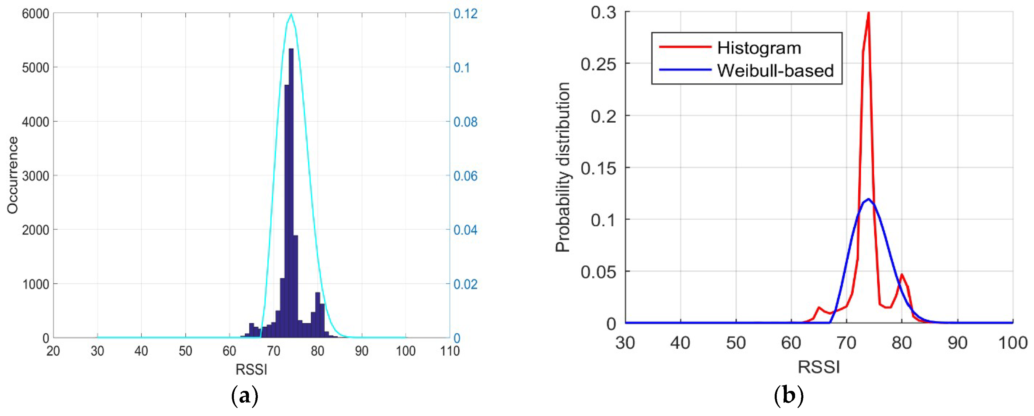
In this study, a sampling test was performed over a period of 12 h in an indoor environment, namely, in the official building of the Central Creative Building covered with Wi-Fi signals, and more than 17,000 RSSI samples were obtained. An interesting distribution can be observed in Figure 1a,b, where the real distribution is almost entirely non-Gaussian and left-skewed. Based on this observation, in this paper, we introduce the Weibull signal model to approximate the RSSI probability distribution of all APs received at each fingerprinting point. The Weibull signal model is a traditional method for modeling the signal strength of propagation radio waves [54]. The corresponding PDF can be expressed as follows:
Accordingly, the cumulative distribution function (CDF) can be expressed as follows:
where is the variable of the function; is the shape parameter; λ is the scale parameter; and is the shift parameter [31,42].
The parameters of the Weibull signal model can be estimated with a limited number of sampled RSSI measurements. The model parameters (, , and ) can be calculated with the following equation [53,55]:
where is the mean value of the RSSI measurements set ; STD denotes the standard deviation; and is the gamma function. The term is an approximation of the expression when [31,47].
Therefore, the distribution probability of each possible RSSI measurement in the fingerprint database can be expressed as follows:
For a fingerprint database measured with the Weibull signal model, we can calculate the probability of occurrence of any RSSI measurement. As the RSSI measurements are integers, the probability for each bin in the fingerprint database can be generated as follows:
where w is the width of the bin, and x is the RSSI value at the left boundary value of bin.
The fingerprinting method using the radio map based on the Weibull–Bayesian density model can be represented by a set of Weibull signal models that simulate the distribution of RSSI measurements. Each Weibull signal model contains three parameters (, , and ) representing the probability distribution of the RSSI measurements between an AP Am and a smartphone at a reference point . The structure of the radio map can be greatly simplified in this case because it requires storing only three parameters of the Weibull function that can restore the complete probability density; in other words, it is not necessary to store probability distribution based on separated RSSI bins as in traditional approaches.
To evaluate the performance of the proposed approach, a fitting experiment was carried out to determinate whether the shape of the Weibull signal model derived from the same RSSI samples can approximate the reference shape derived from a multitude of RSSI measurements acquired over a long recording session. For this purpose, a test was performed over a long recording session in the official building of the Central Creative Building, and 17,874 RSSI samples were acquired. Consequently, considering that the histogram probability distribution derived from the 17,874 RSSI samples collected over a 12-h period was close to the real RSSI probability distribution, we used it as the baseline distribution for the purpose of comparison.
Next, Equations (6)–(10) were used with all of the RSSI samples to calculate the parameters of the Weibull signal mode derived from the entire set of samples as follows: shape = 2.5, scale λ = 8.4428, and shift θ = 67. The estimated Weibull signal mode was then used to compute the PDF, shown as the cyan line in Figure 1a, which was close to the real PDF, as demonstrated in Figure 1a, where the blue colored bars represent the histogram of all RSSI samples. Using Equation (11), we obtained the Weibull-based probability distribution, as shown with the blue line in Figure 1b; the red line is the baseline distribution. Evidently, the shapes of the two lines are similar.
3.2. Fingerprinting Positioning Using the Weibull–Bayesian Density Model
During the position inference phase, the bins were dynamically divided based on the Weibull signal model according to the RSSI measurement of each AP received in real time. Therefore, with the same fingerprinting method, we could compare the probabilities generated from the same data set using three different algorithms: the conventional Bayesian fingerprinting histogram algorithm with static bin; the Weibull bin fingerprinting algorithm based on the Weibull–Bayesian density model with static bin; and the Weibull PDF fingerprinting algorithm based on the Weibull–Bayesian density model with dynamic bin.
The fingerprinting positioning method employed in this paper relied on Bayesian theory and the histogram maximum likelihood algorithm [39]. The principle of this method, which is also called the Bayesian probability algorithm, is to use the conditional probability model for location fingerprinting and the Bayesian inference mechanism to estimate the position of the smartphone [56]. The basic principle can be expressed as follows:
where is a reference point in the fingerprint database; y is the RSSI measurements of the AP received by the smartphone at the anchor point; is the probability that the anchor point is the reference point x when the RSSI measurement is y; is the probability that the RSSI measurement is y at the reference point ; is the probability of a reference point that usually does not consider the difference between the reference points (the default is the equal probability of all reference points); and is the RSSI measurement occurring with the full probability (the default AP is usually mutually independent). From Equation (8), when the value of is maximum, the probability of reference point x occurring when the RSSI value received at the anchor point is y also reaches a maximum. In other words, the best match with the anchor point can be used as the positioning result output. Therefore, the Bayesian probability algorithm is used to find the maximum value of at which x is the positioning result, and the formula can be expressed as follows:
To obtain the maximum value of , we know that and are the same at each fingerprinting point according to the Bayesian theory formula. The maximum value of can be transformed to solve for the maximum value of , which represents the probability of RSSI measurements of each AP being received at reference point x. Because each AP is independent, this method determines the probability product maximum value of the RSSI measurements of each AP, and the formula can be expressed as follows:
where is the total number of AP received by the smartphone at the anchor point; represents the RSSI measurements of the j-th AP received by the smartphone at the anchor point; x is a reference point in the fingerprint database. Therefore, the conditional probability product of all APs at each reference point can be calculated, the maximum probability can be found according to the histogram maximum likelihood algorithm, and the corresponding reference point is the positioning result.
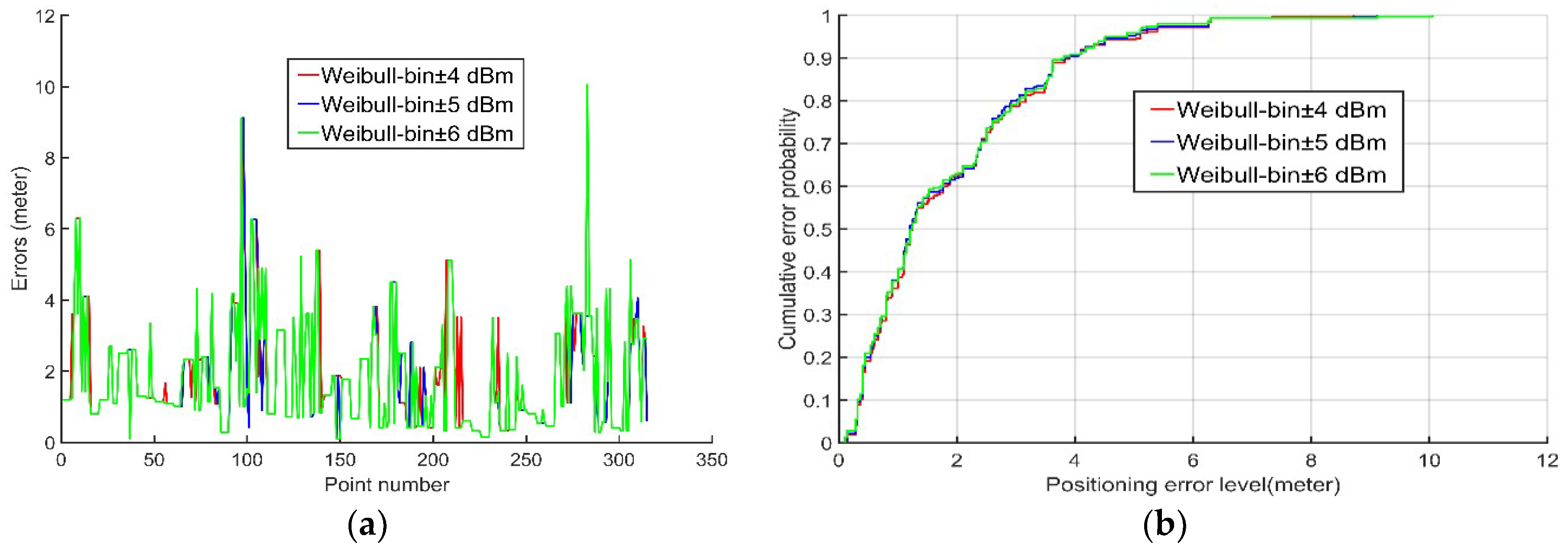
In this paper, the conventional static bin method stored the probability distribution of the RSSI measurements of each AP received at each reference point in a well-defined bin as a radio map. In contrast, the dynamic bin method proposed in this paper added ±B dBm to the RSSI measurements of each AP received during the positioning phase, thereby incorporating a dynamic bin to account for the probability in Equation (5). Accordingly, we calculated a large number of Wi-Fi APs RSSI measurements and found that most of them had a standard deviation between 2 and 3, and 95% of the measurements errors were within twice the standard deviation if the errors followed the Gaussian distribution, according to the theory of the statistics. Thus, the parameter B was given the value of twice the standard deviation. Considering the differences between different APs, an experiment was carried out to compare the positioning accuracy with ±4 dBm, ±5 dBm, and ±6 dBm to identify which would be the best as the value of B. We used the proposed algorithm to calculate the average error and root-mean-square (RMS) error of each RSSI range and plotted the error distribution graphs with ±4 dBm, ±5 dBm, and ±6 dBm in addition to the probability cumulative distribution function of the positioning error. More details about the experiment will be introduced in Section 4.1.
Table 1 and Figure 2 demonstrate that, although they exhibited few differences, the positioning accuracy obtained with ±5 dBm (blue line in Figure 2) were slightly superior to those obtained with both ±4 dBm (red line in Figure 2) and ±6 dBm (green line in Figure 2). Therefore, ±5 dBm proved to be the best B value. The dynamic bin probability of RSSI measurements of each AP received at the anchor point can be expressed as follows:
where is the RSSI value of AP Am received by the smartphone at reference point ; B is the half width of the bin; and are the left and right edges of the dynamic bin, respectively; and represents the probability of occurrence at point when the RSSI value of AP Am is .
The three parameters required by the Weibull–Bayesian density model are stored in the radio map to first model the probability distribution of the RSSI measurements between an AP Am and a smartphone at a reference point and then dynamically calculate the probability value of the bin in real time. This approach constitutes the fingerprinting algorithm based on the Weibull–Bayesian density model with the dynamic bin method proposed in this paper.
4. Experiments and Results
In this positioning experiment, the average error and root-mean-square error in the positioning results of the three algorithms were compared in different actual scenarios. The objective of the experiment was to compare the positioning performance of the two Weibull-based algorithms (Weibull bin and Weibull PDF) with that of the conventional histogram algorithm.
4.1. Experimental Environment and Process
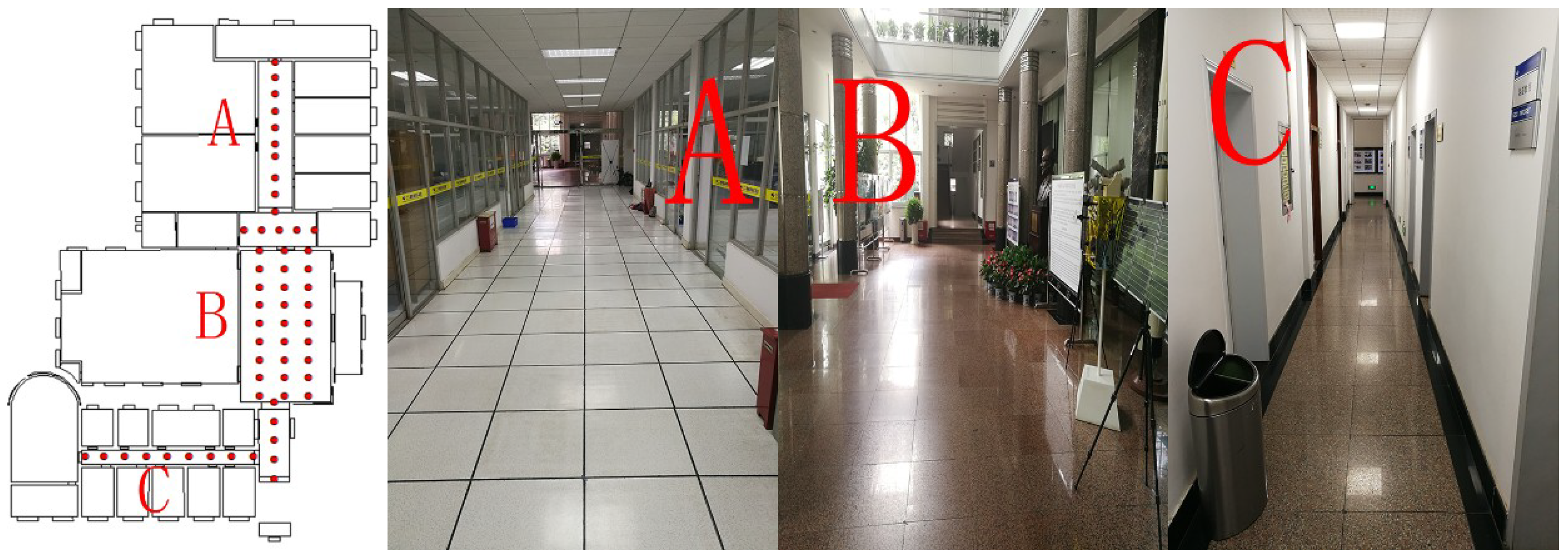
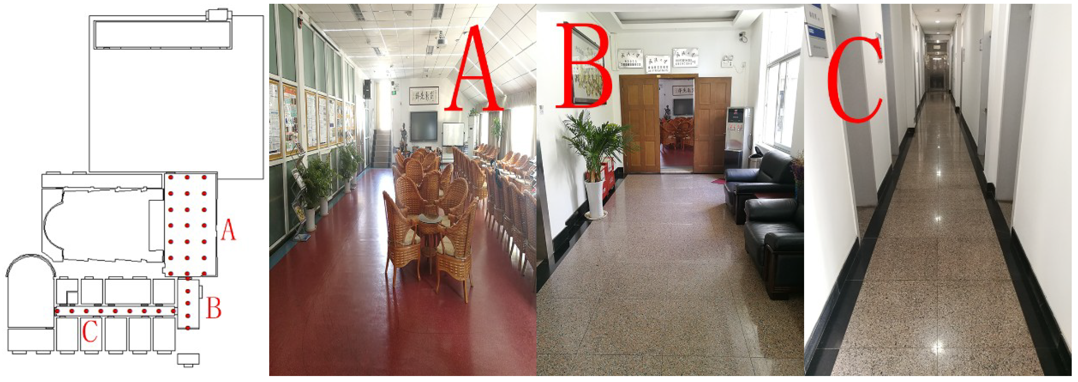
In this experiment, two floor plans were selected to verify the broad applicability of the proposed algorithm in various environments. The two experiments were carried out in public areas on the second and fourth floors, both of which are 53 m by 73 m in size, within the office building of our laboratory. The second floor is mainly composed of a lobby, students’ computer labs, and multiple corridors (see the four maps in Figure 3), whereas the fourth-floor environment is sample and consists only of conference rooms and corridors (see the four maps in Figure 4). Sketches of the floor plans and actual photos are shown in Figure 3 and Figure 4.
Figure 3 and Figure 4 show that our experimental area included most actual scenarios in an office building, including a lobby and a conference room in addition to different types of corridors. In our experiment, 56 reference points were established on a grid map at intervals of 2–3 m in public areas, such as the lobby and corridors on the second floor, and 30 sets of sample data were collected at each reference point to establish the fingerprint database. Subsequently, we randomly selected 43 evaluation points within the experimental area and then measured and recorded the true coordinates of those evaluation points. At each evaluation point, five discontinuous sets of RSSI measurements were collected at different times; as a result, a total of 215 independent sets of data were collected for testing. In the same way, a total of 35 reference points were collected on the fourth floor, and 30 sets of sample data were collected at each fingerprinting point to establish a fingerprint database. A total of 20 evaluation points were selected at random, and five discontinuous sets of RSSI measurements were collected at different times at each evaluation point. In this way, a total of 100 independent sets of data were acquired for testing.
Based upon our experience, it is impractical to dedicate vast amounts of computational and human resources to acquire data at each reference point to train the database. Approximately 20 RSSI samples can be obtained over a one-minute sampling duration, and 30 RSSI samples can be obtained over a 90 s sampling duration. Therefore, we selected 20 samples as a subset of the 30 samples and 30 samples as limited sampling cases for comparison.
4.2. Validation of the Weibull–Bayesian Density Model
Based on the long recording session, 17,874 RSSI samples were acquired in the official building of the Central Creative Building. More fitting experiments were carried out to determine whether the shape of the Weibull signal model derived from a limited subset of RSSI samples could approximate the reference shape derived from a multitude of RSSI measurements acquired over a long recording session. The fitting experiments revealed that the model shape was very similar, even when the number of samples decreased from 10,000 to 30 or 20.
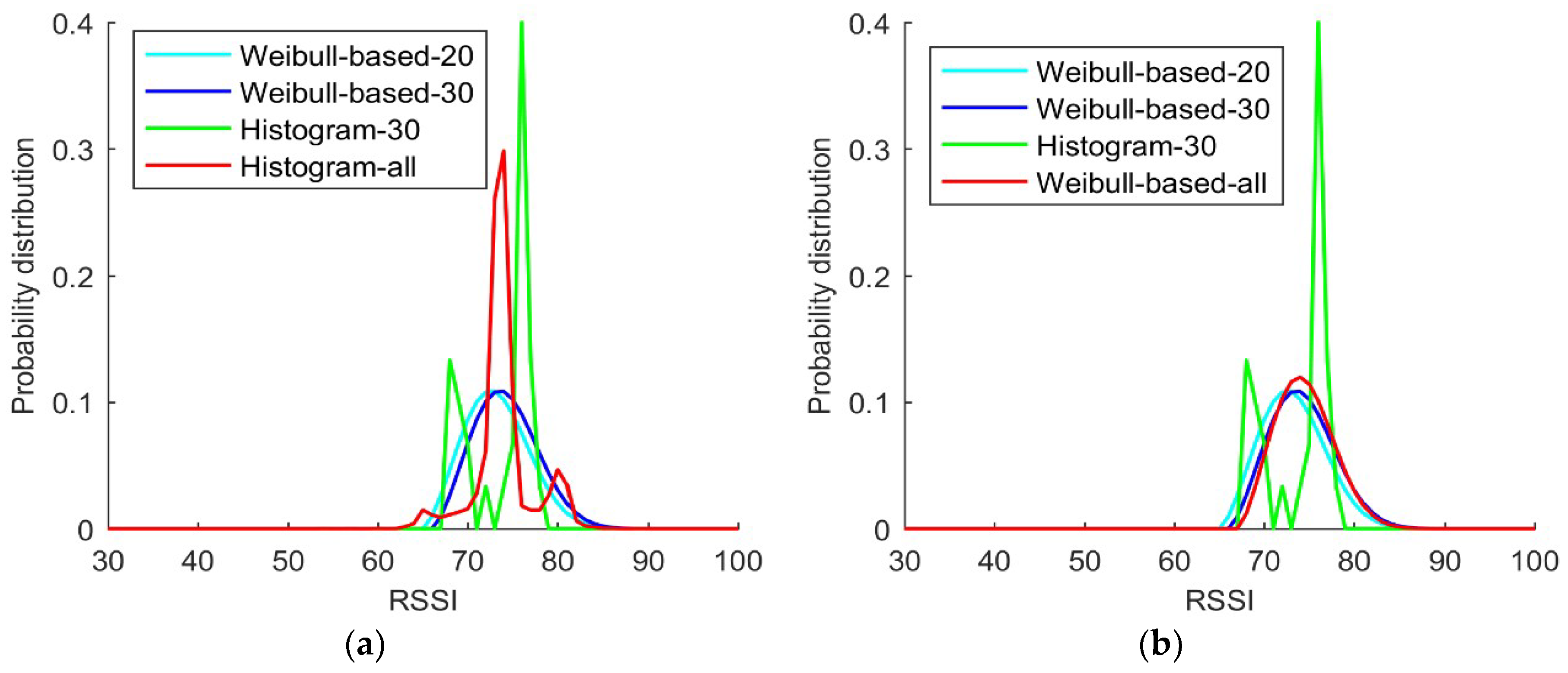
In Figure 5a,b, the blue lines represent the probability distribution derived from a Weibull-based solution using 30 RSSI samples randomly selected from the large data set, while the cyan lines represent the probability distribution derived from a Weibull-based solution using fewer (only 20 out of 30) RSSI samples. The green lines represent the probability distribution derived from the histogram solution for the same data set of 30 RSSI measurement samples, while the red lines in the two figures are different but can be both considered as the baseline distribution according to the comparison in Figure 1. The baseline distribution is the histogram probability distribution derived from all samples in Figure 5a and the probability distributions derived from the Weibull-based solution with all samples in Figure 5b.
Figure 5a,b shows that the shape of the Weibull signal model derived from either 20 or 30 RSSI samples are similar to that of the two baseline distributions. By comparing the probabilities estimated using the conventional Histogram solution with 30 samples with those estimated using the Weibull signal model with 30 samples, it is obvious that the probabilities estimated using the latter are closer to the baseline distribution than is the former. A comparison of the probabilities estimated using the conventional Histogram solution with 30 samples with those estimated using the Weibull signal model with 20 samples reveals that the latter is also better than the former, thereby demonstrating that the Weibull-based solution is more efficient than conventional Histogram solution. Furthermore, the probability distributions estimated with the Weibull-based solutions are significantly better than those obtained from the conventional Histogram solution. Thus, from this experiment, the fingerprint database with the Weibull signal model can improve the efficiency and accuracy of the algorithm.
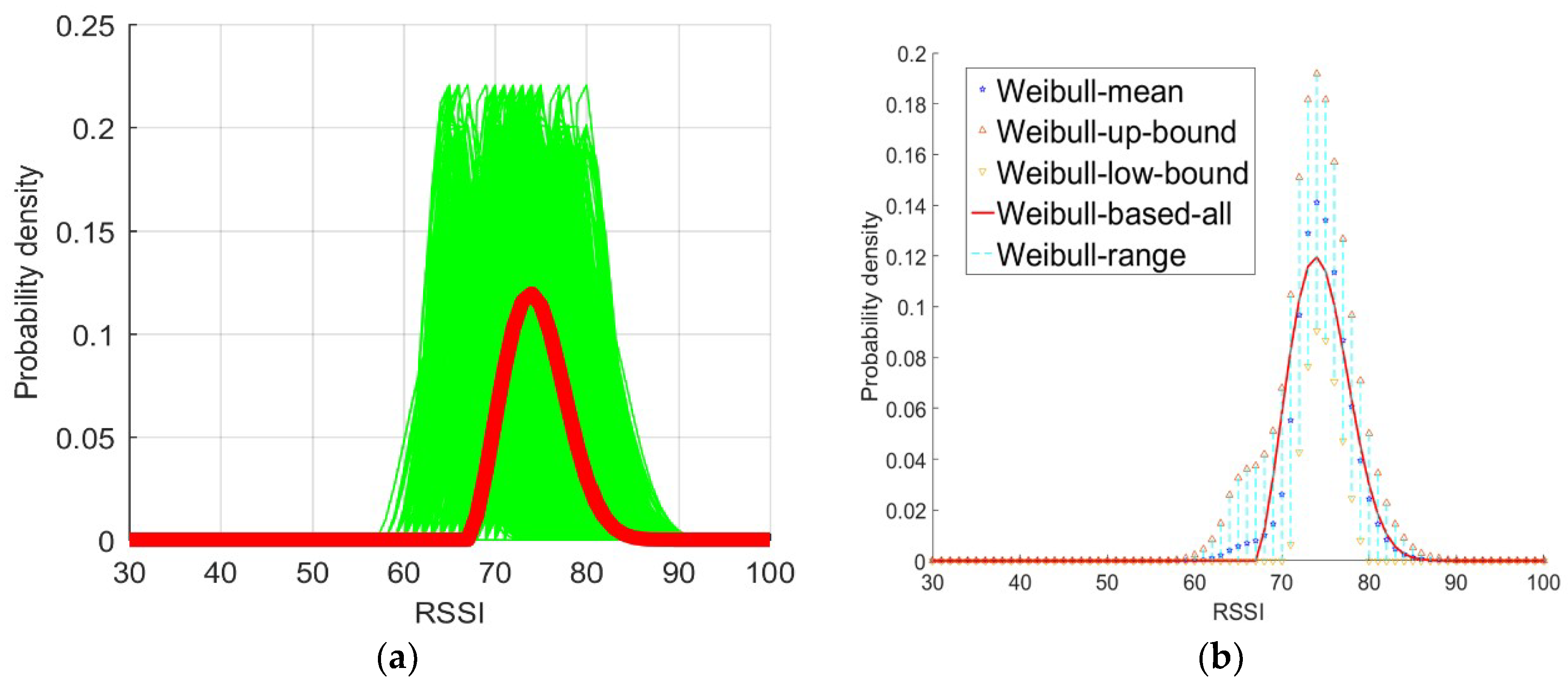
As shown in Figure 6, every set of 30 RSSI samples was taken from the entire sample data set as one session to estimate the parameters of the Weibull signal model (green line in Figure 6a) for the purpose of comparing the resulting probability density with the baseline probability density derived with all samples (red line in Figure 6a). For a more detailed test, the Weibull signal model was used to derive the probability densities and calculate the mean (blue star in Figure 6b) and variance of all sessions. We obtained the ranges of the variables for all sessions where the variable for each session ranges from the mean plus the variance (magenta triangles in Figure 6b) to the mean minus the variance (inverted magenta triangles in Figure 6b). The estimated Weibull signal model with all samples was used to compute the probability density (shown as the red line in Figure 6b). The results intuitively illustrate that the probability density derived with every set of 30 samples was close to the probability density derived with all samples.
It is not difficult to see that the shapes of most Weibull signal model based probability distributions based on the Weibull signal model derived from 30 RSSI samples were close to that of the baseline distribution (the red line in Figure 6). Hence, according to the test, the Weibull signal model based probability distribution derived from 30 RSSI measurement samples effectively approximated the baseline probability distribution.
4.3. Indoor Positioning Performance Evaluation
First, we used all data sets to verify which RSSI range constitutes the best bin for the Weibull PDF algorithm proposed in this paper. Based on the findings shown in Table 1 and Figure 2, we chose ±5 dBm as the RSSI dynamic bin of the Weibull PDF algorithm. In addition, we used three algorithms to calculate the positioning coordinates of all data sets and compared them with the true coordinates recorded to calculate the average error and RMS error of each algorithm. We also plotted the error distribution graph of three algorithms and the probability CDF of the positioning error.
In this study, two dynamic experiments were conducted in which 215 and 100 sets of data were acquired on the second and fourth floors, respectively, within the office building of our laboratory. The test data sets were employed to estimate the position using the histogram algorithm and the two Weibull-based algorithms. All algorithms perform slightly better on the fourth floor than on the second floor. From the actual maps of the two floors (Figure 3 and Figure 4), the result of this experiment could be inferred because the environment on the fourth floor is more open, and the Wi-Fi signal is less disturbed.
The test data sets were applied to estimate the position using the histogram and Weibull-based fingerprint databases. The histogram fingerprint database was generated using Equation (3) with 30 RSSI samples, while the Weibull-based solution was derived from Equation (12) with 20 out of 30 RSSI samples. The experimental results are presented in Table 2 and Table 3. Evidently, the Weibull-based solution performed significantly better than the histogram solution. For a more detailed analysis, the same data sets were utilized to estimate the position using the histogram and Weibull PDF fingerprint databases. The Weibull PDF algorithm clearly performed significantly better than both the conventional histogram algorithm and the Weibull bin algorithm. The accuracy of the Weibull PDF algorithm solution for the data from the second floor was 0.56 m better than that of the histogram solution for the same data set. For the data from the fourth floor, the error of the Weibull PDF algorithm was 0.59 m lower than that of the histogram solution. Compared with the conventional histogram algorithm, the RMS errors of the Weibull PDF algorithm were 20.8% and 35.2% higher in the two different scenarios.
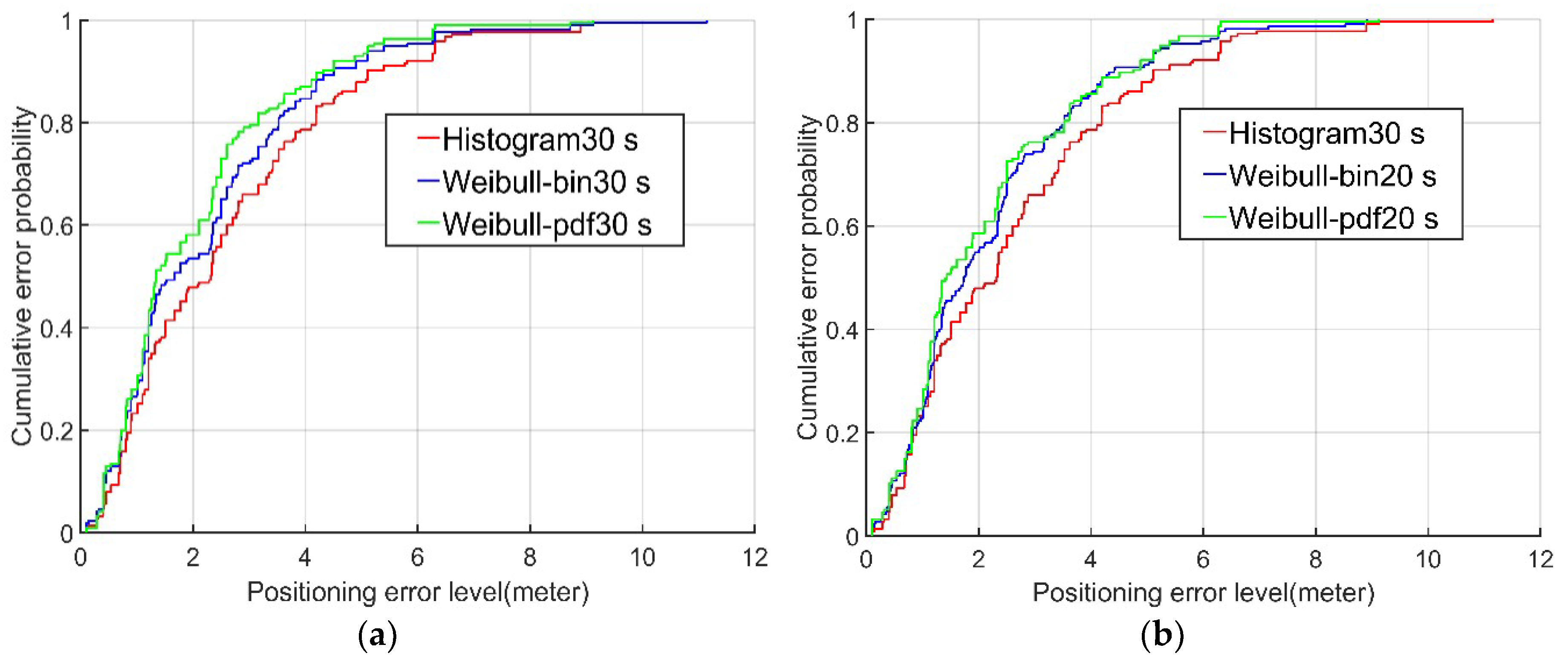
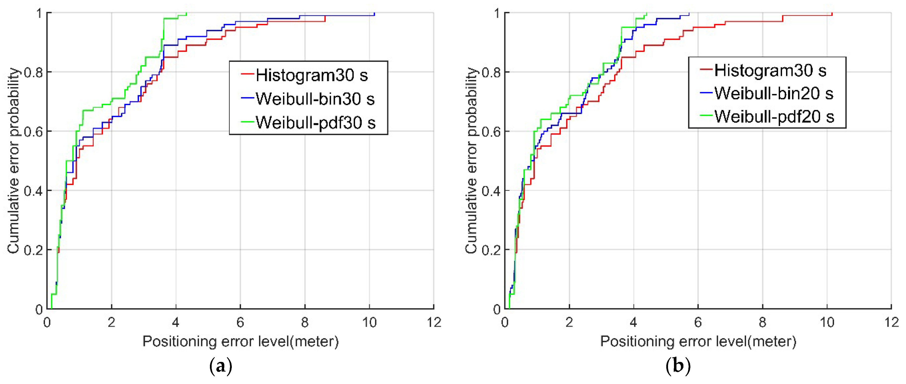
Examining the cumulative probability distributions in the error graph, the positioning results for the data from the second and fourth floors using the Weibull PDF algorithm (green lines in Figure 7 and Figure 8) were 60% and 70%, respectively, when the positioning error was less than 2 m. In contrast, the corresponding results using the conventional histogram algorithm (red lines in Figure 7 and Figure 8) and the Weibull bin algorithm (blue lines in Figure 7 and Figure 8) were only approximately 50% and 60%, respectively, when the positioning error was less than 2 m. When the cumulative probability of the positioning error was 95%, the positioning errors of the Weibull PDF algorithm were 5.22 m and 3.63 m on the second and fourth floors, respectively, while the positioning errors of the conventional histogram algorithm were only 6.3 m and 6.18 m, respectively, and those of the Weibull bin algorithm were 5.81m and 5.45 m, respectively. It is obvious from this that the Weibull PDF algorithm proposed in this paper had the highest accuracy. Even when the established fingerprint database contained only 20 RSSI samples, the Weibull PDF algorithm performed better than the conventional histogram algorithm with 30 RSSI samples.
In general, the three algorithms utilized in the experiment exhibited some points with larger errors, although the Weibull PDF algorithm always performed significantly better than the conventional histogram algorithm and Weibull bin algorithm. The mean errors of the proposed algorithm were 2.03 m and 1.37 m for the two actual scenes on the second and fourth floors, respectively, and 90% and 98% of the positioning errors were within 4 m. In addition, compared with the conventional histogram algorithm, the RMS errors of the Weibull PDF algorithm were 20.8% and 35.2% higher in the two different scenarios. These findings reveal that the proposed algorithm improved not only the positioning accuracy but also the acquisition and calculation efficiency of the fingerprint database.
5. Conclusions
The utility of radio-signal-based indoor positioning has recently received increased attention from researchers. Accordingly, in this paper, a method is proposed based on the Bayesian fingerprinting positioning method with Wi-Fi RSSI observables that optimizes the radio map learning and position inference phase to enhance its usability. During the radio map learning phase, the proposed method uses a Weibull–Bayesian density model to represent the PDF of Wi-Fi RSSI observables, which can be calculated with fewer samples. Moreover, the proposed method can calculate the PDF with a higher accuracy than the traditional histogram method. The parameterized Weibull model can greatly reduce both the amount of necessary fieldwork and the cost of the radio map learning phase. Furthermore, the method proposed herein effectively resolves the contradiction between large sampling statistics and data collection efficiency. During the position inference phase, the proposed method calculates the posterior probability using the Bayesian density model and a dynamically defined run-time bin according to real-time RSSI observables rather than the probability distribution of predefined RSSI bins as is accomplished in traditional methods. When implemented on an Android smartphone in different indoor environments, the proposed method enhanced the usability of Wi-Fi Bayesian fingerprinting positioning by requiring a smaller number (i.e., one-third) of signal observables and improved the positioning accuracy by 19–32% in different building environments compared with the classical histogram-based method. In general, the new method proposed in this paper exhibits good prospects.
However, the presented results are only for Wi-Fi fingerprinting positioning, and the proposed method has not been integrated with pedestrian dead reckoning (PDR) or other localization sources; hence, the positioning accuracy is not fully up-to-date. In the future, we will conduct additional studies on multisource integrated positioning. For instance, the fusion of Wi-Fi fingerprinting with PDR and maps will result in a better positioning accuracy.
Author Contributions
Conceptualization, Z.L. and J.L.; Methodology, Z.L., F.Y., X.N., and L.L.; Software, Z.L. and F.Y.; Validation, Z.L. and F.Y.; Formal Analysis, Z.L., J.L., F.Y., X.N., and L.L.; Investigation, Z.L.; Resources, J.L.; Data Curation, Z.L., J.L., F.Y., X.N., and L.L.; Writing—Original Draft Preparation, Z.L. and J.L.; Writing—Review and Editing, Z.L., J.L., X.N., L.L., Z.W., and R.C.; Visualization, Z.L. and F.Y.; Supervision, Z.W. and R.C.; Project Administration, J.L.; Funding Acquisition, J.L.
Funding
This study was supported in part by the National Key Research Development Program of China with project No. 2016YFB0502204, the Natural Science Fund of China with Project No. 41874031, the Natural Science Fund of China with Project No. 61872431, the Technology Innovation Program of Hubei Province with Project No. 2018AAA070, and the Natural Science Fund of Hubei Province with Project No. 2018CFA007.
Conflicts of Interest
The authors declare no conflict of interest.
References
- He, S.; Chan, S.H.G. Wi-Fi fingerprint-based indoor positioning: Recent advances and comparisons. IEEE Commun. Surv. Tutor. 2017, 18, 466–490. [Google Scholar] [CrossRef]
- Global Indoor Location Market Analysis (2017–2023). Available online: https://www.reportlinker.com/p05207399/Global-Indoor-Location-Market-Analysis.html (accessed on 23 November 2017).
- Moreira, A.; Silva, I.; Meneses, F.; Nicolau, M.J.; Pendão, C.; Torres-Sospedra, J. Multiple simultaneous Wi-Fi measurements in fingerprinting indoor positioning. In Proceedings of the 2017 International Conference on Indoor Positioning and Indoor Navigation (IPIN), Sapporo, Japan, 18–21 September 2017. [Google Scholar]
- Jovan Powar, C.G.; Harle, R. Assessing the Impact of Multi-Channel BLE Beacons on Fingerprint-based Positioning. In Proceedings of the 2017 International Conference on Indoor Positioning and Indoor Navigation (IPIN), Sapporo, Japan, 18–21 September 2017. [Google Scholar]
- Jiménez, A.R.; Seco, F. Combining RSS-based trilateration methods with radio-tomographic imaging: Exploring the capabilities of long-range RFID systems. In Proceedings of the 2015 International Conference on Indoor Positioning and Indoor Navigation (IPIN), Banff, AB, Canada, 13–16 October 2015; pp. 13–16. [Google Scholar]
- Jiménez, A.R.; Zampella, F.; Seco, F. Light-Matching: A new Signal of Opportunity for Pedestrian Indoor Navigation. In Proceedings of the International Conference on Indoor Positioning and Indoor Navigation (IPIN), Montbeliard-Belfort, France, 28–31 October 2013; pp. 777–786. [Google Scholar]
- Antigny, N.; Servières, M.; Renaudin, V. Pedestrian Track Estimation with Handheld Monocular Camera and Inertial-Magnetic Sensor for Urban Augmented Reality. In Proceedings of the 2017 International Conference on Indoor Positioning and Indoor Navigation (IPIN), Sapporo, Japan, 18–21 September 2017. [Google Scholar]
- Hanley, D.; Faustino, A.; Zelman, S.; Degenhardt, D.; Bretl, T. MagPIE: A Dataset for Indoor Positioning with Magnetic Anomalies. In Proceedings of the 2017 International Conference on Indoor Positioning and Indoor Navigation (IPIN), Sapporo, Japan, 18–21 September 2017. [Google Scholar]
- Vaughan-Nichols, S.J. Will mobile computing’s future be location, location, location? Computer 2009, 42, 14–17. [Google Scholar] [CrossRef]
- Torres-Sospedra, J.; Jiménez, A.R.; Moreira, A.; Lungenstrass, T.; Lu, W.; Knauth, S.; Mendoza-Silva, G.M.; Seco, F.; Pérez-Navarro, A.; Nicolau, M.J.; et al. Off-Line Evaluation of Mobile-Centric Indoor Positioning Systems: The Experiences from the 2017 IPIN Competition. Sensors 2018, 18, 487. [Google Scholar] [CrossRef] [PubMed]
- Davidson, P.; Piche, R. A survey of selected indoor positioning methods for smartphones. IEEE Commun. Surv. Tutor. 2017, 19, 1347–1370. [Google Scholar] [CrossRef]
- Günther, A.; Hoene, C. Measuring Round Trip Times to Determine the Distance Between WLAN Nodes. In Proceedings of the 4th IFIP-TC6 International Conference on Networking Technologies, Services, and Protocols; Performance of Computer and Communication Networks; Mobile and Wireless Communication Systems, Waterloo, ON, Canada, 2–6 May 2005; pp. 768–779. [Google Scholar]
- Li, Q.; Li, W.; Sun, W.; Wang, J.; Li, J. Wi-Fi indoor localization algorithm based on rssi and assistant nodes collaboration. J. Electron. Measur. Instrum. 2016, 30, 794–802. [Google Scholar]
- Fang, S.; Cheng, Y.; Chien, Y. Exploiting Sensed Radio Strength and Precipitation for Improved Distance Estimation. IEEE Sens. J. 2018, 18, 6863–6873. [Google Scholar] [CrossRef]
- Whitehouse, K.; Karlof, C.; Culler, D. A practical evaluation of radio signal strength for ranging-based localization. ACM SIGMOBILE Mob. Comput. Commun. Rev. 2007, 11, 41–52. [Google Scholar] [CrossRef]
- Pivato, P.; Palopoli, L.; Petri, D. Accuracy of RSS-Based Centroid Localization Algorithms in an Indoor Environment. IEEE Trans. Instrum. Meas. 2011, 60, 3451–3460. [Google Scholar] [CrossRef] [Green Version]
- Laitinen, H.; Juurakko, S.; Lahti, T.; Korhonen, R.; Lahteenmaki, J. Experimental Evaluation of Location Methods Based on Signal-Strength Measurements. IEEE Trans. Veh. Technol. 2007, 56, 287–296. [Google Scholar] [CrossRef]
- Le Dortz, N.; Gain, F.; Zetterberg, P. WiFi Fingerprint Indoor Positioning System Using Probability Distribution Comparison. In Proceedings of the IEEE International Conference on Acoustics, Speech and Signal Processing (ICASSP), Kyoto, Japan, 25–30 March 2012; pp. 2301–2304. [Google Scholar]
- Chen, B.; Liu, R.; Chen, Y.; Liu, J.; Jiang, X.; Liu, D. WiFi fingerprint based self-adaptive indoor localization in the dynamic environment. Chin. J. Sens. Actuators 2015, 28, 729–738. [Google Scholar]
- Llombart, M.; Ciurana, M.; Barcelo-Arroyo, F. On the Scalability of a Novel WLAN Positioning System based on Time of Arrival Measurements. In Proceedings of the 5th Workshop on Positioning, Navigation and Communication, Hannover, Germany, 27 March 2006; pp. 15–21. [Google Scholar]
- Tang, J.; Chen, Y.; Chen, L.; Liu, J.; Hyyppä, J.; Kukko, A.; Kaartinen, H.; Hyyppä, H.; Chen, R. Fast fingerprint database maintenance for indoor positioning based on UGV SLAM. Sensors 2015, 15, 5311–5330. [Google Scholar] [CrossRef] [PubMed]
- Kim, K.; Cho, S. Modular Bayesian Networks with Low-Power Wearable Sensors for Recognizing Eating Activities. Sensors 2017, 17, 2877. [Google Scholar] [Green Version]
- Berkvens, R.; Peremans, H.; Weyn, M. Conditional Entropy and Location Error in Indoor Localization Using Probabilistic Wi-Fi Fingerprinting. Sensors 2016, 16, 1636. [Google Scholar] [CrossRef] [PubMed]
- Yu, F.; Jiang, M.; Liang, J.; Qin, X.; Hu, M.; Peng, T.; Hu, X. Expansion RSS-based Indoor Localization Using 5G WiFi Signal. In Proceedings of the IEEE International Conference on Computational Intelligence and Communication Networks, Bhopal, India, 14–16 November 2014; pp. 510–514. [Google Scholar]
- Cramariuc, A.; Huttunen, H.; Lohan, S. Clustering benefits in mobile-centric WiFi positioning in multi-floor buildings. In Proceedings of the 2016 International Conference on Localization and GNSS (ICL-GNSS), Barcelona, Spain, 28–30 June 2016. [Google Scholar]
- Marques, N.; Meneses, F.; Moreira, A. Combining similarity functions and majority rules for multi-building, multi-floor, WiFi Positioning. In Proceedings of the 2012 International Conference on Indoor Positioning and Indoor Navigation (IPIN), Sydney, Australia, 13–15 November 2012. [Google Scholar]
- He, C.; Guo, S.; Wu, Y.; Yang, Y. A novel radio map construction method to reduce collection effort for indoor localization. Measurement 2016, 94, 423–431. [Google Scholar] [CrossRef]
- Racko, J.; Machaj, J.; Brida, P. Wi-Fi fingerprint radio map creation by using interpolation. Procedia Eng. 2017, 192, 753–758. [Google Scholar] [CrossRef]
- Ferris, B.; Hahnel, D.; Fox, D. Gaussian Processes for Signal Strength-Based Location Estimation. In Proceedings of the Robotics Science and Systems, Ann Arbor, MI, USA, 20–22 June 2006. [Google Scholar]
- Ferris, B.; Fox, D.; Lawrence, D. WiFi-SLAM Using Gaussian Process Latent Variable Models. In Proceedings of the National Conference on Artificial Intelligence, Hyderabad, India, 8 January 2007; pp. 2480–2485. [Google Scholar]
- Liu, J.; Chen, R.; Pei, L.; Chen, W.; Tenhunen, T.; Kuusniemi, H.; Kröger, T.; Chen, Y. Accelerometer assisted robust wireless signal positioning based on a hidden Markov model. In Proceedings of the IEEE/ION Position, Location and Navigation Symposium, Indian Wells, CA, USA, 4–6 May 2010; pp. 488–497. [Google Scholar]
- Kushki, A.; Plataniotis, K.N.; Venetsanopoulos, A.N. Kernel-based positioning in wireless local area networks. IEEE Trans. Mob. Comput. 2007, 6, 689–705. [Google Scholar] [CrossRef]
- Kaemarungsi, K.; Krishnamurthy, P. Properties of Indoor Received Signal Strength for WLAN Location Fingerprinting. In Proceedings of the First Annual International Conference on Mobile and Ubiquitous Systems: Networking and Services, Boston, MA, USA, 26 August 2004; pp. 14–23. [Google Scholar]
- Li, B.; Wang, Y.; Lee, H.K.; Dempster, A.; Rizos, C. Method for yielding a database of location fingerprints in WLAN. IEE Proc. Commun. 2005, 152, 580–586. [Google Scholar] [CrossRef]
- Badawy, O.M.; Hasan, M.A.B. Decision Tree Approach to Estimate User Location in WLAN based on Location Fingerprinting. In Proceedings of the National Radio Science Conference, Cairo, Egypt, 13–15 March 2007; pp. 1–10. [Google Scholar]
- Yan, Y.; Tan, Q.; Li, P.; Yang, H. Study on WIFI Indoor Location Techniques based on Android. In Proceedings of the 2017 International Conference on Computer Systems, Electronics and Control (ICCSEC), Dalian, China, 25–27 December 2017. [Google Scholar]
- Chen, L.; Li, B.; Zhao, K.; Rizos, C.; Zheng, Z. An improved algorithm to generate a Wi-Fi fingerprint database for indoor positioning. Sensors 2013, 13, 11085–11096. [Google Scholar] [CrossRef] [PubMed]
- Wu, D.; Xu, Y.; Ma, L. Research on RSS based Indoor Location Method. In Proceedings of the 2009 Pacific-Asia Conference on Knowledge Engineering and Software Engineering, Shenzhen, China, 19–20 December 2009; pp. 205–208. [Google Scholar]
- Youssef, M.A.; Agrawala, A.; Shankar, A.U. WLAN Location Determination via Clustering and Probability Distributions. In Proceedings of the First IEEE International Conference on Pervasive Computing and Communications, Fort Worth, TX, USA, 26 March 2003; pp. 143–150. [Google Scholar]
- Liu, J.; Chen, R.; Chen, Y.; Pei, L.; Chen, L. iParking: An intelligent indoor location-based smartphone parking service. Sensors 2012, 12, 14612–14629. [Google Scholar] [CrossRef] [PubMed]
- Pei, L.; Liu, J.; Guinness, R.; Chen, Y.; Kuusniemi, H.; Chen, R. Using LS-SVM based motion recognition for smartphone indoor wireless positioning. Sensors 2012, 12, 6155–6175. [Google Scholar] [CrossRef] [PubMed]
- Pei, L.; Chen, R.; Liu, J.; Kuusniemi, H.; Tenhunen, T.; Chen, Y. Using inquiry-based bluetooth RSSI probability distributions for indoor positioning. J. Glob. Position. Syst. 2010, 9, 122–130. [Google Scholar]
- Sun, Y.; Xu, Y.; Ma, L.; Deng, Z. KNN-FCM Hybrid Algorithm for Indoor Location in WLAN. In Proceedings of the 2nd International Conference on Power Electronics and Intelligent Transportation System (PEITS), Shenzhen, China, 19–20 December 2009; pp. 251–254. [Google Scholar]
- Machaj, J.; Piché, R.; Brida, P. Rank Based Fingerprinting Algorithm for Indoor Positioning. In Proceedings of the 2011 International Conference on Indoor Positioning and Indoor Navigation, Guimaraes, Portugal, 21–23 September 2011. [Google Scholar]
- Torres-Sospedra, J.; Montoliu, R.; Trilles, S.; Belmonte, Ó.; Huerta, J. Comprehensive Analysis of Distance and Similarity Measures for Wi-Fi Fingerprinting Indoor Positioning Systems. Expert Syst. Appl. 2015, 42, 9263–9278. [Google Scholar] [CrossRef] [Green Version]
- Zhang, W.; Hua, X.; Qiu, W.; Xue, W.; Zhou, D. A new combinatorial optimization algorithm for WiFi positioning. Eng. Surv. Mapp. 2017, 26, 14–18. [Google Scholar]
- Escobar, M.D.; West, M. Bayesian density estimation and inference using mixtures. J. Am. Stat. Assoc. 1995, 90, 577–588. [Google Scholar] [CrossRef]
- Argiento, R.; Guglielmi, A.; Pievatolo, A. Bayesian density estimation and model selection using nonparametric hierarchical mixtures. Comput. Stat. Data Anal. 2010, 54, 816–832. [Google Scholar] [CrossRef] [Green Version]
- Dunson, D.B.; Pillai, N.; Park, J.-H. Bayesian density regression. J. R. Stat. Soc. Series B 2007, 69, 163–183. [Google Scholar] [CrossRef] [Green Version]
- Kaemarungsi, K. Distribution of WLAN Received Signal Strength Indication for Indoor Location Determination. In Proceedings of the 1st International Symposium on Wireless Pervasive Computing, Phuket, Thailand, 16–18 January 2006. [Google Scholar]
- Youssef, M.A. HORUS: A WLAN-Based Indoor Location Determination System. Ph.D. Thesis, University of Maryland, College Park, MD, USA, 2004. [Google Scholar]
- Xiang, Z.; Song, S.; Chen, J.; Wang, H.; Huang, J.; Gao, X. A wireless LAN-based indoor positioning technology. IBM J. Res. Dev. 2004, 48, 617–626. [Google Scholar] [CrossRef] [Green Version]
- Liu, J.; Chen, R.; Pei, L.; Guinness, R.; Kuusniemi, H. A hybrid smartphone indoor positioning solution for mobile LBS. Sensors 2012, 12, 17208–17233. [Google Scholar] [CrossRef] [PubMed]
- Sagias, N.C.; Karagiannidis, G.K. Gaussian class multivariate weibull distributions: Theory and applications in fading channels. IEEE Trans. Inf. Theory 2005, 51, 3608–3619. [Google Scholar] [CrossRef]
- Papoulis, A. Probability, random variables, and stochastic processes. Phys. Today 2001, 20, 135. [Google Scholar] [CrossRef]
- Roos, T.; Myllymäki, P.; Tirri, H.; Misikangas, P.; Sievänen, J. Probabilistic approach to WLAN user location estimation. Int. J. Wirel. Inf. Networks 2002, 9, 155–164. [Google Scholar] [CrossRef]
Figure 1.
Comparison of probability distributions: (a) a typical comparison of the RSSI probability density derived with the histogram ( = 74, STD = 3.186) and Weibull signal model (cyan line, referring to the right axis); (b) Weibull-based probability distribution ( = 2.5, λ = 8.4428, θ = 67) with 17,874 samples (blue line) vs. the histogram probability distribution with 17,874 samples (red line). The RSSI is in the unit of –dBm in this paper.

Figure 2.
The (a) positioning error and (b) cumulative distribution function (CDFs) of different RSSI ranges.
Figure 2.
The (a) positioning error and (b) cumulative distribution function (CDFs) of different RSSI ranges.

Figure 3.
Second-floor plan: Area (A) is the corridor between the students’ computer labs, which is characterized by a large flow of people, and is large, and has a complex Wi-Fi signal environment. Area (B) is a large, spacious lobby with fewer Wi-Fi signals. Area (C) is the corridor between the teacher’s office characterized by a simple physical environment and a simple Wi-Fi signal environment. The area in the first picture (where there is no reference point) is private and cannot be tested.

Figure 4.
Fourth-floor plan: Area (A) is a large conference room that is irregular and has fewer Wi-Fi signals. Areas (B,C) are different types of corridors with simple physical environments and simple Wi-Fi signal environments. The area in the first picture (where there is no reference point) is private and cannot be tested.

Figure 5.
Comparison of probability distributions: (a) Weibull-based probability distribution with 20 samples (cyan line) vs. Weibull-based probability distribution with 30 samples (blue line) vs. histogram probability distribution with 30 samples (green line) vs. histogram probability distribution with all samples (red line). (b) Weibull-based probability distribution with 20 samples (cyan line) vs. Weibull-based probability distribution with 30 samples (blue line) vs. histogram probability distribution with 30 samples (green line) vs. Weibull-based probability distribution with all samples (red line).

Figure 6.
(a) Probability densities estimated using all samples (red line) and each probability density function (PDF) estimated with the Weibull signal model for all sessions with sets of 30 RSSI measurement samples (cluster of green lines). (b) The cyan dashed line connects the mean of the value of all sessions plus the variance of the value of all sessions (magenta triangles), the mean of the value of all sessions (blue stars), and the mean of the value of all sessions minus the variance of the value of all sessions (inverted magenta triangles); the red line is the baseline distribution.

Figure 7.
The (a,b) CDFs of the three algorithms on the second floor.

Figure 8.
The (a,b) CDFs of the three algorithms on the fourth floor.


Table 1.
Comparison of errors in different received signal strength indication (RSSI) ranges.
| ±4 dBm | ±5 dBm | ±6 dBm | |
|---|---|---|---|
| RMS | 2.41 | 2.38 | 2.38 |
| Mean error (m) | 1.85 | 1.81 | 1.81 |
| 95% error (m) | 5.17 | 4.5 | 4.69 |
Table 2.
Comparison of errors in the three algorithms on the second floor.
| Histogram 30 s | Weibull bin | Weibull PDF | |||
|---|---|---|---|---|---|
| 20 s | 30 s | 20 s | 30 s | ||
| RMS | 3.27 | 2.79 | 2.9 | 2.65 | 2.59 |
| Mean error (m) | 2.59 | 2.21 | 2.25 | 2.1 | 2.03 |
| 95% error (m) | 6.3 | 5.39 | 5.81 | 5.39 | 5.22 |
Table 3.
Comparison of errors in the three algorithms on the fourth floor.
| Histogram 30 s | Weibull bin | Weibull PDF | |||
|---|---|---|---|---|---|
| 20 s | 30 s | 20 s | 30 s | ||
| RMS | 2.87 | 2.12 | 2.61 | 1.94 | 1.86 |
| Mean error (m) | 1.96 | 1.54 | 1.79 | 1.42 | 1.37 |
| 95% error (m) | 6.18 | 4.19 | 5.45 | 3.84 | 3.63 |
© 2018 by the authors. Licensee MDPI, Basel, Switzerland. This article is an open access article distributed under the terms and conditions of the Creative Commons Attribution (CC BY) license (http://creativecommons.org/licenses/by/4.0/).
Share and Cite
MDPI and ACS Style
Li, Z.; Liu, J.; Yang, F.; Niu, X.; Li, L.; Wang, Z.; Chen, R. A Bayesian Density Model Based Radio Signal Fingerprinting Positioning Method for Enhanced Usability. Sensors 2018, 18, 4063. https://doi.org/10.3390/s18114063
AMA Style
Li Z, Liu J, Yang F, Niu X, Li L, Wang Z, Chen R. A Bayesian Density Model Based Radio Signal Fingerprinting Positioning Method for Enhanced Usability. Sensors. 2018; 18(11):4063. https://doi.org/10.3390/s18114063
Chicago/Turabian StyleLi, Zheng, Jingbin Liu, Fan Yang, Xiaoguang Niu, Leilei Li, Zemin Wang, and Ruizhi Chen. 2018. "A Bayesian Density Model Based Radio Signal Fingerprinting Positioning Method for Enhanced Usability" Sensors 18, no. 11: 4063. https://doi.org/10.3390/s18114063
Note that from the first issue of 2016, this journal uses article numbers instead of page numbers. See further details here.