Comparing the Potential of Multispectral and Hyperspectral Data for Monitoring Oil Spill Impact

 , , ,
, , ,
Abstract
:
1. Introduction
2. Data and Methods
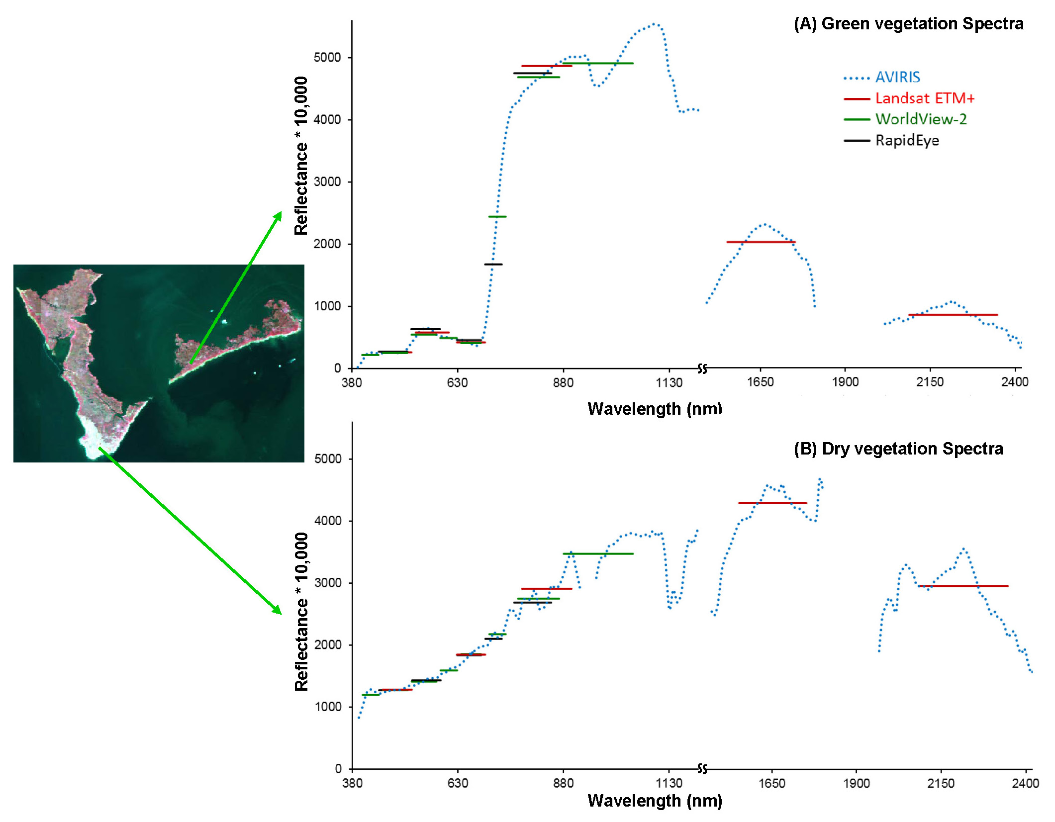
2.1. Study Area
2.2. Image Data and Preprocessing
2.3. Methods
2.3.1. AVIRIS Hyperspectral Data
2.3.2. Multispectral Sensor Data
2.3.3. Selection of Oiled and Oil-Free Areas
2.3.4. Detection of Vegetation Stress
3. Results
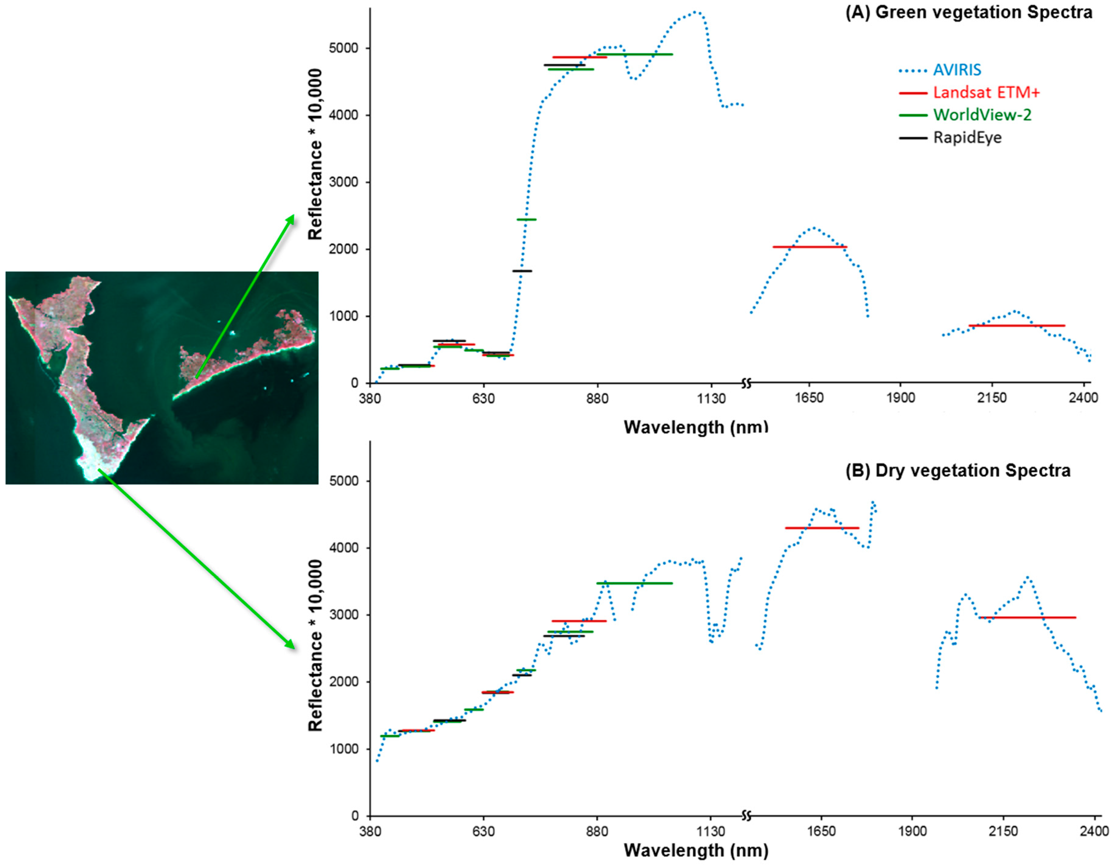
3.1. AVIRIS Hyperspectral Data
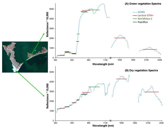
3.1.1. Spectral Resolution
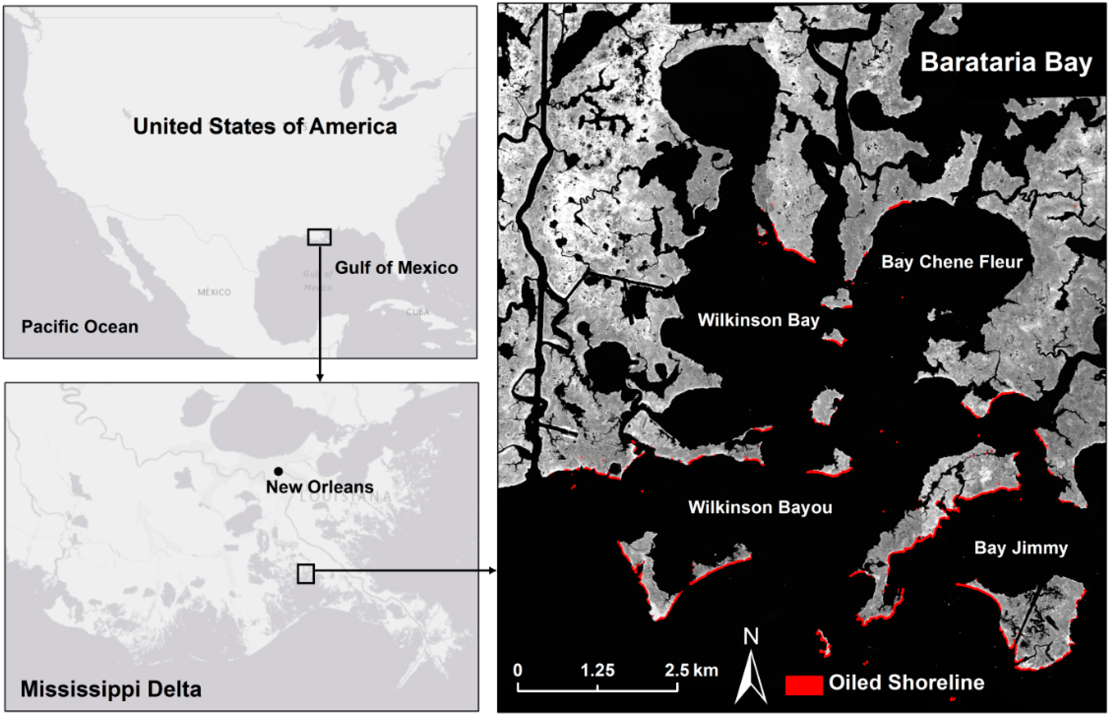
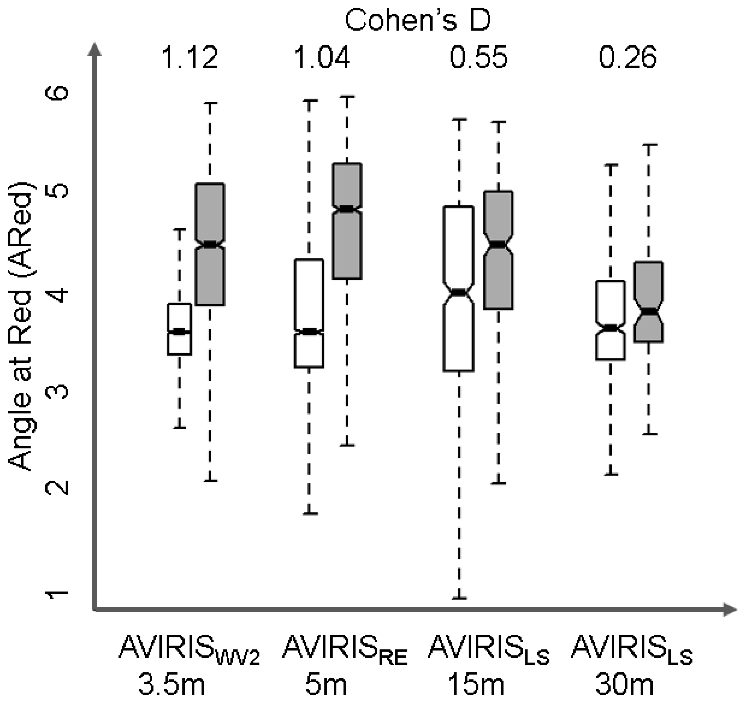
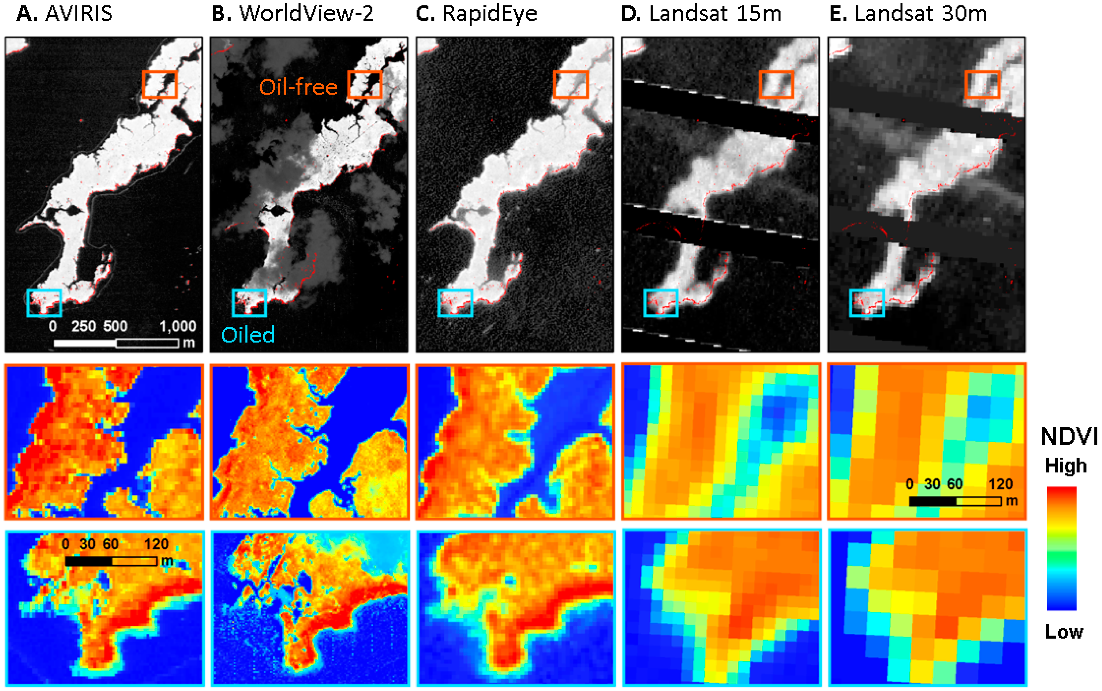
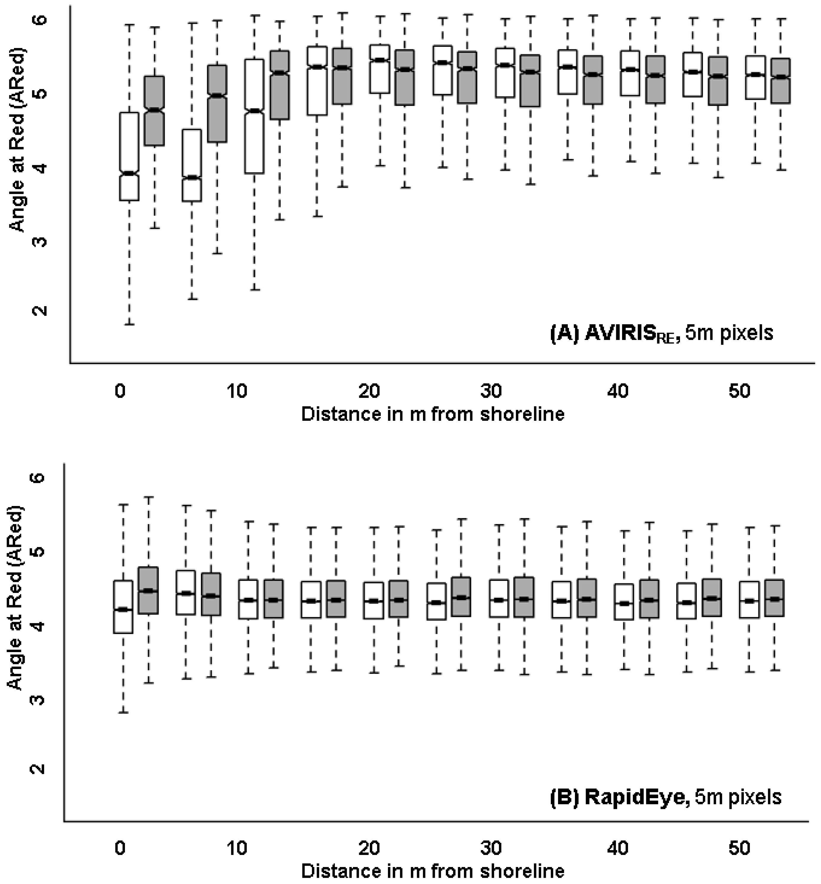
3.1.2. Spatial Resolution
3.2. Multispectral Data
4. Discussion
4.1. Spectral Resolution
4.2. Spatial Resolution
4.3. Sensor Signal-to-Noise Ratio (SNR)
4.4. Timing of Image Acquisition
5. Conclusions
Acknowledgments
Author Contributions
Conflict of Interest
References
- Reimold, R.J.; Hardisky, M.A. Nonconsumptive use of values of wetlands. In Wetland Functions and Values; Greeson, P.E., Clark, J.R., Clark, J.E., Eds.; American Water Resources Association: Minneapolis, MN, USA, 1979; pp. 558–564. [Google Scholar]
- Barbier, E.B.; Hacker, S.D.; Kennedy, C.; Koch, E.W.; Stier, A.C.; Silliman, B.R. The value of estuarine and coastal ecosystem services. Ecol. Monogr. 2011, 81, 169–193. [Google Scholar] [CrossRef]
- Barbier, E.B.; Koch, E.W.; Silliman, B.R.; Hacker, S.D.; Wolanski, E.; Primavera, J.; Granek, E.F.; Polasky, S.; Aswani, S.; Cramer, L.A.; et al. Coastal Ecosystem-Based Management with Nonlinear Ecological Functions and Values. Science 2008, 319, 321–323. [Google Scholar] [CrossRef] [PubMed]
- Kirwan, M.L.; Megonigal, J.P. Tidal wetland stability in the face of human impacts and sea-level rise. Nature 2013, 504, 53–60. [Google Scholar] [CrossRef] [PubMed]
- Liquete, C.; Piroddi, C.; Drakou, E.G.; Gurney, L.; Katsanevakis, S.; Charef, A.; Egoh, B. Current Status and Future Prospects for the Assessment of Marine and Coastal Ecosystem Services: A Systematic Review. PLoS ONE 2013, 8, e67737. [Google Scholar] [CrossRef] [PubMed] [Green Version]
- Temmerman, S.; Meire, P.; Bouma, T.J.; Herman, P.M.J.; Ysebaert, T.; De Vriend, H.J. Ecosystem-based coastal defence in the face of global change. Nature 2013, 504, 79–83. [Google Scholar] [CrossRef] [PubMed]
- Duarte, C.M.; Losada, I.J.; Hendriks, I.E.; Mazarrasa, I.; Marba, N. The role of coastal plant communities for climate change mitigation and adaptation. Nature Clim. Chang. 2013, 3, 961–968. [Google Scholar] [CrossRef]
- Möller, I.; Kudella, M.; Rupprecht, F.; Spencer, T.; Paul, M.; van Wesenbeeck, B.K.; Wolters, G.; Jensen, K.; Bouma, T.J.; Miranda-Lange, M.; et al. Wave attenuation over coastal salt marshes under storm surge conditions. Nat. Geosci. 2014, 7, 727–731. [Google Scholar] [CrossRef]
- Blum, M.D.; Roberts, H.H. Drowning of the Mississippi Delta due to insufficient sediment supply and global sea-level rise. Nat. Geosci. 2009, 2, 488–491. [Google Scholar] [CrossRef]
- Blum, M.D.; Roberts, H.H. The Mississippi Delta Region: Past, Present, and Future. AREPS 2012, 40, 655–683. [Google Scholar] [CrossRef]
- Day, J.; Britsch, L.; Hawes, S.; Shaffer, G.; Reed, D.; Cahoon, D. Pattern and process of land loss in the Mississippi Delta: A Spatial and temporal analysis of wetland habitat change. Estuaries 2000, 23, 425–438. [Google Scholar] [CrossRef]
- Conner, W.; Day, J., Jr.; Baumann, R.; Randall, J. Influence of hurricanes on coastal ecosystems along the northern Gulf of Mexico. Wetlands Ecol. Manag. 1989, 1, 45–56. [Google Scholar] [CrossRef]
- Gundlach, E.R.; Hayes, M.O. Vulnerability of coastal environments to oil spill impacts. Mar. Technol. Soc. J. 1978, 12, 18–27. [Google Scholar]
- Burk, J.C. A Four Year Analysis of Vegetation Following an Oil Spill in a Freshwater Marsh. J. Appl. Ecol. 1977, 14, 515–522. [Google Scholar] [CrossRef]
- Hester, M.W.; Mendelssohn, I.A. Long-term recovery of a Louisiana brackish marsh plant community from oil-spill impact: Vegetation response and mitigating effects of marsh surface elevation. Mar. Environ. Res. 2000, 49, 233–254. [Google Scholar] [CrossRef]
- Lin, Q.; Mendelssohn, I.A. Impacts and recovery of the Deepwater Horizon Oil Spill on vegetation structure and function of coastal salt marshes in the northern gulf of Mexico. Environ. Sci. Technol. 2012, 46, 3737–3743. [Google Scholar] [CrossRef] [PubMed]
- Ramseur, J.L. Oil Spills in U.S. Coastal Waters: Background, Governance, and Issues for Congress; Congressional Research Service: Washington, DC, USA, 2010.
- Moss, L. The 13 largest oil spills in history. In Mother Nature Network; Narrative Content Group: Atlanta, GA, USA, 2010. [Google Scholar]
- Judy, C.R.; Graham, S.A.; Lin, Q.; Hou, A.; Mendelssohn, I.A. Impacts of Macondo oil from Deepwater Horizon spill on the growth response of the common reed Phragmites australis: A mesocosm study. Mar. Pollut. Bull. 2014, 79, 69–76. [Google Scholar] [CrossRef] [PubMed]
- Khanna, S.; Santos, M.J.; Ustin, D.S.L.; Koltunov, A.; Kokaly, R.F.; Roberts, D.A. Detection of salt marsh vegetation stress after the Deepwater Horizon BP oil spill along the shoreline of gulf of Mexico using AVIRIS data. PLoS ONE 2013, 8, e78989. [Google Scholar] [CrossRef] [PubMed]
- Lin, Q.; Mendelssohn, I.A.; Graham, S.A.; Hou, A.; Fleeger, J.W.; Deis, D.R. Response of salt marshes to oiling from the Deepwater Horizon spill: Implications for plant growth, soil surface-erosion, and shoreline stability. Sci. Total Environ. 2016, 557–558, 369–377. [Google Scholar] [CrossRef] [PubMed]
- Mishra, D.R.; Cho, H.J.; Ghosh, S.; Fox, A.; Downs, C.; Merani, P.B.T.; Kirui, P.; Jackson, N.; Mishra, S. Post-spill state of the marsh: Remote estimation of the ecological impact of the Gulf of Mexico oil spill on Louisiana Salt Marshes. Remote Sens. Environ. 2012, 118, 176–185. [Google Scholar] [CrossRef]
- Silliman, B.R.; van de Koppel, J.; McCoy, M.W.; Diller, J.; Kasozi, G.N.; Earl, K.; Adams, P.N.; Zimmerman, A.R. Degradation and resilience in Louisiana salt marshes after the BP–Deepwater Horizon oil spill. Proc. Natl. Acad. Sic. USA 2012, 109, 11234–11239. [Google Scholar] [CrossRef] [PubMed]
- Wiens, J.A. Review of an ecosystem services approach to assessing the impacts of the Deepwater Horizon Oil Spill in the Gulf of Mexico. Fisheries 2015, 40, 86. [Google Scholar] [CrossRef]
- Ko, J.Y.; Day, J.W. A review of ecological impacts of oil and gas development on coastal ecosystems in the Mississippi Delta. Ocean Coast. Manag. 2004, 47, 597–623. [Google Scholar] [CrossRef]
- Pezeshki, S.R.; Hester, M.W.; Lin, Q.; Nyman, J.A. The effects of oil spill and clean-up on dominant US Gulf coast marsh macrophytes: A review. Environ. Pollut. 2000, 108, 129–139. [Google Scholar] [CrossRef]
- Smith, C.J.; Delaune, R.D.; Patrick, W.H.; Fleeger, J.W. Impact of dispersed and undispersed oil entering a gulf coast salt marsh. Environ. Toxicol. Chem. 1984, 3, 609–616. [Google Scholar] [CrossRef]
- Pezeshki, S.R.; DeLaune, R.D. United States Gulf of Mexico Coastal Marsh Vegetation Responses and Sensitivities to Oil Spill: A Review. Environments 2015, 2, 586–607. [Google Scholar] [CrossRef]
- Lin, Q.; Mendelssohn, I.A. A comparative investigation of the effects of south Louisiana crude oil on the vegetation of fresh, brackish and salt marshes. Mar. Pollut. Bull. 1996, 32, 202–209. [Google Scholar] [CrossRef]
- Kenworthy, W.J.; Durako, M.J.; Fatemy, S.M.R.; Valavi, H.; Thayer, G.W. Ecology of seagrasses in northeastern Saudi Arabia one year after the Gulf War oil spill. Mar. Pollut. Bull. 1993, 27, 213–222. [Google Scholar] [CrossRef]
- Khanna, S.; Santos, M.; Koltunov, A.; Shapiro, K.; Lay, M.; Ustin, S. Marsh Loss Due to Cumulative Impacts of Hurricane Isaac and the Deepwater Horizon Oil Spill in Louisiana. Remote Sens. 2017, 9, 169. [Google Scholar] [CrossRef]
- Jackson, J.B.C.; Cubit, J.D.; Keller, B.D.; Batista, V.; Burns, K.; Caffey, H.M.; Caldwell, R.L.; Garrity, S.D.; Getter, C.D.; Gonzalez, C.; et al. Ecological effects of a major oil spill on Panamanian coastal marine communities. Science 1989, 243, 37–44. [Google Scholar] [CrossRef] [PubMed]
- Walker, D.A.; Webber, P.J.; Everett, K.R.; Brown, J. Effects of Crude and Diesel Oil Spills on Plant Communities at Prudhoe Bay, Alaska, and the Derivation of Oil Spill Sensitivity Maps. Arctic 1978, 31, 242–259. [Google Scholar] [CrossRef]
- Houborg, R.; Soegaard, H.; Boegh, E. Combining vegetation index and model inversion methods for the extraction of key vegetation biophysical parameters using Terra and Aqua MODIS reflectance data. Remote Sens. Environ. 2007, 106, 39–58. [Google Scholar] [CrossRef]
- Jurgens, C. The modified normalized difference vegetation index (mNDVI) a new index to determine frost damages in agriculture based on Landsat TM data. Int. J. Remote Sens. 1997, 18, 3583–3594. [Google Scholar] [CrossRef]
- Peñuelas, J.; Gamon, J.A.; Griffin, K.L.; Field, C.B. Assessing community type, plant biomass, pigment composition, and photosynthetic efficiency of aquatic vegetation from spectral reflectance. Remote Sens. Environ. 1993, 46, 110–118. [Google Scholar] [CrossRef]
- Ustin, S.L.; Gitelson, A.A.; Jacquemoud, S.; Schaepman, M.; Asner, G.P.; Gamon, J.A.; Zarco-Tejada, P. Retrieval of foliar information about plant pigment systems from high resolution spectroscopy. Remote Sens. Environ. 2009, 113, S67–S77. [Google Scholar] [CrossRef] [Green Version]
- Zarco-Tejada, P.J.; Rueda, C.A.; Ustin, S.L. Water content estimation in vegetation with MODIS reflectance data and model inversion methods. Remote Sens. Environ. 2003, 85, 109–124. [Google Scholar] [CrossRef]
- Gitelson, A.; Merzlyak, M.N. Spectral reflectance changes associated with autumn senescence of Aesculus-hippocastanum L. and Acer-platanoides L. leaves—Spectral features and relation to chlorophyll estimation. J. Plant Physiol. 1994, 143, 286–292. [Google Scholar] [CrossRef]
- Gitelson, A.A.; Merzlyak, M.N. Remote estimation of chlorophyll content in higher plant leaves. Int. J. Remote Sens. 1997, 18, 2691–2697. [Google Scholar] [CrossRef]
- Fensholt, R.; Sandholt, I. Derivation of a shortwave infrared water stress index from MODIS near- and shortwave infrared data in a semiarid environment. Remote Sens. Environ. 2003, 87, 111–121. [Google Scholar] [CrossRef]
- Gao, B.C. NDWI—Normalized difference water index for remote sensing of vegetation liquid water from space. Remote Sens. Environ. 1996, 58, 257–266. [Google Scholar] [CrossRef]
- Hunt, E.R.; Rock, B.N. Detection of changes in leaf water content using near-infrared and middle-infrared reflectances. Remote Sens. Environ. 1989, 30, 43–54. [Google Scholar]
- Khanna, S.; Palacios-Orueta, A.; Whiting, M.L.; Ustin, S.L.; Riano, D.; Litago, J. Development of angle indexes for soil moisture estimation, dry matter detection and land-cover discrimination. Remote Sens. Environ. 2007, 109, 154–165. [Google Scholar] [CrossRef]
- Lillesand, T.M.; Kiefer, R.W.; Chipman, J.W. Remote Sensing and Image Interpretation; John Wiley & Sons, Inc.: New York, NY, USA, 2004. [Google Scholar]
- Richardson, A.J.; Wiegand, C.L. Distinguishing Vegetation from Soil Background Information. Photogramm. Eng. Remote Sens. 1977, 43, 1541–1552. [Google Scholar]
- Tucker, C.J. Red and photographic infrared linear combinations for monitoring vegetation. Remote Sens. Environ. 1979, 8, 127–150. [Google Scholar] [CrossRef]
- Palacios-Orueta, A.; Whiting, M.L.; Ustin, S.L.; Litago, J.; Garcia, M.; Khanna, S. Cotton phenology analysis with the new remote sensing spectral angle indexes AS1 and AS2. In Proceedings of the International Conference on Agricultural Engineering, Crete, Greece, 23–25 June 2008. [Google Scholar]
- Li, L.; Ustin, S.L.; Lay, M. Application of AVIRIS data in detection of oil-induced vegetation stress and cover change at Jornada, New Mexico. Remote Sens. Environ. 2005, 94, 1–16. [Google Scholar] [CrossRef]
- Boochs, F.; Kupfer, G.; Dockter, K.; Kühbauch, W. Shape of the red edge as vitality indicator for plants. Int. J. Remote Sens. 1990, 11, 1741–1753. [Google Scholar] [CrossRef]
- Carter, G.A. Responses of Leaf Spectral Reflectance to Plant Stress. Am. J. Bot. 1993, 80, 239–243. [Google Scholar] [CrossRef]
- Bammel, B.H.; Birnie, R.W. Spectral Reflectance Response of Big Sagebrush to Hydrocarbon-Induced Stress in the Bighorn Basin, Wyoming; American Society for Photogrammetry and Remote Sensing: Bethesda, MD, USA, 1994; Volume 60. [Google Scholar]
- Rosso, P.H.; Pushnik, J.C.; Lay, M.; Ustin, S.L. Reflectance properties and physiological responses of Salicornia virginica to heavy metal and petroleum contamination. Environ. Pollut. 2005, 137, 241–252. [Google Scholar] [CrossRef] [PubMed]
- Van Der Meer, F.; Van Dijk, P.; Van Der Werff, H.; Yang, H. Remote sensing and petroleum seepage: A review and case study. Terra Nova 2002, 14, 1–17. [Google Scholar] [CrossRef]
- Yang, H.; Zhang, J.; Van der Meer, F.; Kroonenberg, S.B. Geochemistry and field spectrometry for detecting hydrocarbon microseepage. Terra Nova 1998, 10, 231–235. [Google Scholar] [CrossRef]
- Wilson, C.A.; Allison, M.A. An equilibrium profile model for retreating marsh shorelines in southeast Louisiana. Estuar. Coast. Shelf Sci. 2008, 80, 483–494. [Google Scholar] [CrossRef]
- Gosselink, J.G.; Pendleton, E.C. The Ecology of Delta Marshes of Coastal Louisiana: A Community Profile; U.S. Fish and Wildlife Service: Washington DC, USA, 1984; p. 156.
- Jones, C.E.; Minchew, B.; Holt, B.; Hensley, S. Studies of the Deepwater Horizon Oil Spill With the UAVSAR Radar. In Monitoring and Modeling the Deepwater Horizon Oil Spill: A Record-Breaking Enterprise; AGU: Washington, DC, USA, 2011; Volume 195, pp. 33–50. [Google Scholar]
- Liu, P.; Li, X.; Qu, J.J.; Wang, W.; Zhao, C.; Pichel, W. Oil spill detection with fully polarimetric UAVSAR data. Mar. Pollut. Bull. 2011, 62, 2611–2618. [Google Scholar] [CrossRef] [PubMed]
- Michel, J.; Owens, E.H.; Zengel, S.; Graham, A.; Nixon, Z.; Allard, T.; Holton, W.; Reimer, P.D.; Lamarche, A.; White, M.; et al. Extent and degree of shoreline oiling: Deepwater Horizon oil spill, Gulf of Mexico, USA. PLoS ONE 2013, 8, e65087. [Google Scholar] [CrossRef] [PubMed]
- Ramsey, E., III; Rangoonwala, A.; Suzuoki, Y.; Jones, C.E. Oil detection in a coastal marsh with polarimetric Synthetic Aperture Radar (SAR). Remote Sens. 2011, 3, 2630–2662. [Google Scholar] [CrossRef] [Green Version]
- Kokaly, R.F.; Couvillion, B.R.; Holloway, J.M.; Roberts, D.A.; Ustin, S.L.; Peterson, S.H.; Khanna, S.; Piazza, S.C. Spectroscopic remote sensing of the distribution and persistence of oil from the Deepwater Horizon spill in Barataria Bay marshes. Remote Sens. Environ. 2013, 129, 210–230. [Google Scholar] [CrossRef]
- Kokaly, R.F.; Heckman, D.; Holloway, J.; Piazza, S.C.; Couvillion, B.R.; Steyer, G.D.; Mills, C.T.; Hoefen, T.M. Shoreline surveys of Oil-Impacted Marsh in Southern Louisiana, July to August 2010; U.S. Geological Survey: Reston, VA, USA, 2011.
- Platt, R.V.; Goetz, A.F.H. A Comparison of AVIRIS and Landsat for Land Use Classification at the Urban Fringe. Photogram. Eng. Remote Sens. 2004, 70, 813–819. [Google Scholar] [CrossRef]
- Miecznik, G.; Grabowska, D. Worldview-2 bathymetric capabilities. In Proceedings of the Algorithms and Technologies for Multispectral, Hyperspectral, and Ultraspectral Imagery XVIII, Baltimore, MD, USA, 23–27 April 2012; pp. 83901J-1–83901J-10. [Google Scholar]
- Brunn, A.; Freedman, E.; Fleming, R. New Resampling Kernel and Its Effect on RapidEye Imagery. Available online: http://www.serioussciencellc.com/files/CMTF_JACIE2013.pdf (accessed on 9 February 2014).
- Reulke, R.; Weichelt, H. SNR Evaluation of the RapidEye Space-borne Cameras. Photogramm.-Fernerkund.-Geoinf. 2012, 2012, 29–38. [Google Scholar] [CrossRef]
- Mika, A.M. Three Decades of Landsat Instruments. Photogramm. Eng. Remote Sens. 1997, 63, 839–852. [Google Scholar]
- Richter, R.; Schläpfer, D. Geo-atmospheric processing of airborne imaging spectrometry data. Part 2: Atmospheric/topographic correction. Int. J. Remote Sens. 2002, 23, 2631–2649. [Google Scholar] [CrossRef]
- Ben-Dor, E.; Kindel, B.C.; Patkin, K. A comparison between six model-based methods to retrieve surface reflectance and water vapor content from hyperspectral data: A case study using synthetic AVIRIS data. In Proceedings of the International Conference on Optics and Optoelectronics, Dehradun, India, 12–15 December 2005. [Google Scholar]
- Koltunov, A.; Ben-Dor, E.; Ustin, S.L. Image construction using multitemporal observations and Dynamic Detection Models. Int. J. Remote Sens. 2008, 30, 57–83. [Google Scholar] [CrossRef]
- Koltunov, A.; Ustin, S.L.; Quayle, B.; Schwind, B. GOES Early Fire Detection (GOES-EFD) system prototype. In Proceedings of the ASPRS 2012 Anuual Conference, Sacramento, CA, USA, 19–23 March 2012. [Google Scholar]
- Khanna, S.; Santos, M.J.; Ustin, S.L.; Haverkamp, P.J. An integrated approach to a biophysiologically based classification of floating aquatic macrophytes. Int. J. Remote Sens. 2011, 32, 1067–1094. [Google Scholar] [CrossRef]
- Clark, R.N.; Roush, T.L. Reflectance spectroscopy—Quantitative analysis techniques for remote sensing applications. J. Geophys. Res. Solid Earth 1984, 89, 6329–6340. [Google Scholar] [CrossRef]
- Rosenfield, G.H.; Fitzpatrick-Lins, K. A coefficient of agreement as a measure of thematic classification accuracy. Photogramm. Eng. Remote Sens. 1986, 52, 223–227. [Google Scholar]
- Story, M.; Congalton, R.G. Accuracy assessment—A user's perspective (map interpretation). Photogramm. Eng. Remote Sens. 1986, 52, 397–399. [Google Scholar]
- Laben, C.A.; Brower, B.V. Process for Enhancing the Spatial Resolution of Multispectral Imagery Using Pan-Sharpening. U.S. Patent 6,011,875, 4 January 2000. [Google Scholar]
- Mitsch, W.J.; Gosselink, J.G. Wetlands; John Wiley & Sons, Inc.: New York, NY, USA, 2007. [Google Scholar]
- Hardisky, M.A.; Klemas, V.; Smart, R.M. The influence of soil-salinity, growth form, and leaf moisture on the spectral radiance of Spartina-alterniflora canopies. Photogramm. Eng. Remote Sens. 1983, 49, 77–83. [Google Scholar]
- Palacios-Orueta, A.; Khanna, S.; Litago, J.; Whiting, M.L.; Ustin, S.L. Assessment of NDVI and NDWI spectral indices using MODIS time series analysis and development of a new spectral index based on MODIS shortwave infrared bands. In Proceedings of the 1st international conference of remote sensing and geoinformation processing, Trier, Germany, 7–9 September 2005; pp. 207–209. [Google Scholar]
- Cohen, J. Statistical Power Analysis for the Behavioral Sciences; Academic Press: New York, NY, USA, 1969. [Google Scholar]
- Cohen, J. Statistical Power Analysis for the Behavioral Sciences, 2nd ed.; Lawrence Earlbaum Associates: Hillsdale, NJ, USA, 1988. [Google Scholar]
- Khanna, S.; Santos, M.J.; Hestir, E.L.; Ustin, S.L. Plant community dynamics relative to the changing distribution of a highly invasive species, Eichhornia crassipes: A remote sensing perspective. Biol. Invasions 2012, 14, 717–733. [Google Scholar] [CrossRef]
- Alves, T.M.; Kokinou, E.; Zodiatis, G. A three-step model to assess shoreline and offshore susceptibility to oil spills: The South Aegean (Crete) as an analogue for confined marine basins. Mar. Pollut. Bull. 2014, 86, 443–457. [Google Scholar] [CrossRef] [PubMed]
- Alves, T.M.; Kokinou, E.; Zodiatis, G.; Lardner, R.; Panagiotakis, C.; Radhakrishnan, H. Modelling of oil spills in confined maritime basins: The case for early response in the Eastern Mediterranean Sea. Environ. Pollut. 2015, 206, 390–399. [Google Scholar] [CrossRef] [PubMed]
- Al-Awadhi, J.M.; Omar, S.A.; Misak, R.F. Land degradation indicators in Kuwait. LDD 2005, 16, 163–176. [Google Scholar] [CrossRef]
- Cross, A.M. Monitoring marine oil pollution using AVHRR data : Observation of the coast of Kuwait and Saudi Arabia during January 1991. Int. J. Remote Sens. 1992, 13, 781–788. [Google Scholar] [CrossRef]
- Bianchi, R.; Cavalli, R.M.; Marino, C.M.; Pignatti, S.; Poscolieri, M. Use of airborne hyperspectral images to assess the spatial distribution of oil spilled during the Trecate blow-out (Northern Italy). In Proceedings of the Remote Sensing for Agriculture, Forestry, and Natural Resources, Paris, France, 26–28 September 1995; pp. 352–362. [Google Scholar]
- Salem, F.; Kafatos, M. Hyperspectral Image Analysis for Oil Spill Mitigation. In Proceedings of the 22nd Asian Conference on Remote Sensing, Singapore, 5–9 November 2001. [Google Scholar]
- Brekke, C.; Solberg, A.H.S. Oil spill detection by satellite remote sensing. Remote Sens. Environ. 2005, 95, 1–13. [Google Scholar] [CrossRef]
- DiGiacomo, P.M.; Washburn, L.; Holt, B.; Jones, B.H. Coastal pollution hazards in southern California observed by SAR imagery: Stormwater plumes, wastewater plumes, and natural hydrocarbon seeps. Mar. Pollut. Bull. 2004, 49, 1013–1024. [Google Scholar] [CrossRef] [PubMed]
- Simecek-Beatty, D.; Clemente-Colón, P. Locating a sunken vessel using SAR imagery: Detection of oil spilled from the SS Jacob Luckenbach. Int. J. Remote Sens. 2004, 25, 2233–2241. [Google Scholar] [CrossRef]
- Peterson, S.H.; Roberts, D.A.; Beland, M.; Kokaly, R.F.; Ustin, S.L. Oil detection in the coastal marshes of Louisiana using MESMA applied to band subsets of AVIRIS data. Remote Sens. Environ. 2015, 159, 222–231. [Google Scholar] [CrossRef]
- Cho, H.; Lee, K.-S. Comparison between Hyperspectral and Multispectral Images for the Classification of Coniferous Species. Korean J. Remote Sens. 2014, 30, 25–36. [Google Scholar] [CrossRef]
- Govender, M.; Chetty, K.; Naiken, V.; Bulcock, H. A comparison of satellite hyperspectral and multispectral remote sensing imagery for improved classification and mapping of vegetation. Water SA 2008, 34, 147–154. [Google Scholar]
- Santos, M.J.; Hestir, E.L.; Khanna, S.; Ustin, S.L. Image spectroscopy and stable isotopes elucidate functional dissimilarity between native and nonnative plant species in the aquatic environment. New Phytol. 2012, 193, 683–695. [Google Scholar] [CrossRef] [PubMed]
- Mumby, P.J.; Edwards, A.J. Mapping marine environments with IKONOS imagery: Enhanced spatial resolution can deliver greater thematic accuracy. Remote Sens. Environ. 2002, 82, 248–257. [Google Scholar] [CrossRef]
- Underwood, E.; Ustin, S.; Ramirez, C. A Comparison of Spatial and Spectral Image Resolution for Mapping Invasive Plants in Coastal California. Environ. Manage. 2007, 39, 63–83. [Google Scholar] [CrossRef] [PubMed]
- Teillet, P.M.; Staenz, K.; William, D.J. Effects of spectral, spatial, and radiometric characteristics on remote sensing vegetation indices of forested regions. Remote Sens. Environ. 1997, 61, 139–149. [Google Scholar] [CrossRef]
- Van Wagtendonk, J.W.; Root, R.R.; Key, C.H. Comparison of AVIRIS and Landsat ETM+ detection capabilities for burn severity. Remote Sens. Environ. 2004, 92, 397–408. [Google Scholar] [CrossRef]
- Asner, G.P.; Heidebrecht, K.B. Spectral unmixing of vegetation, soil and dry carbon cover in arid regions: Comparing multispectral and hyperspectral observations. Int. J. Remote Sens. 2002, 23, 3939–3958. [Google Scholar] [CrossRef]
- Bach, H.; Mauser, W. Improvements of plant parameter estimations with hyperspectral data compared to multispectral data. In Proceedings of the Remote Sensing of Vegetation and Sea, Taormina, Italy, 23–26 September 1996; pp. 59–67. [Google Scholar]
- Lee, K.-S.; Cohen, W.B.; Kennedy, R.E.; Maiersperger, T.K.; Gower, S.T. Hyperspectral versus multispectral data for estimating leaf area index in four different biomes. Remote Sens. Environ. 2004, 91, 508–520. [Google Scholar] [CrossRef]
- Paul, F.; Huggel, C.; Kääb, A.; Kellenberger, T.; Maisch, M. Comparison of TM-Derived Glacier Areas with Higher Resolution Data Sets. In Proceedings of the EARSeL-LISSIG-Workshop Observing our Cryosphere from Space, Bern, Switzerland, 11–13 March 2002. [Google Scholar]
- Shapiro, K.; Khanna, S.; Ustin, S.L. Differential Impact and Recovery of Oil-induced Stress on Three Diverse Sites in the Gulf of Mexico due to the BP Deepwater Horizon Oil Spill. In Proceedings of the Ecological Society of America, Sacramento, CA, USA, 10–14 August 2014. [Google Scholar]


| AVIRIS | WorldView2 | Rapid Eye | Landsat ETM+ | |
|---|---|---|---|---|
| Bandwidth | 10–15 nm | 40–180 nm | 40–90 nm | 60–260 nm |
| Spatial resolution | 3.5 m | 2 m | 5 m | 15 m, 30 m |
| Radiometric resolution | 16-bit | 11-bit | 16-bit | 8-bit |
| Time of acquisition | 19 September 2010 | 8 September 2010 | 8 October 2010 | 13 September 2010 |
| Signal-to-noise ratio | 800–1200 [64] | 250–500 [65] | 90–140 [66,67] | 20–55 [64,68] |
| Cloud cover | 0% | 30% | 0% | 0% |
| Inputs | Formula | Relevance | References | Index Calculated Using Sensors |
|---|---|---|---|---|
| Normalized Difference Vegetation Index (NDVI) | Index of green plant cover and LAI | [46,47] | AVIRIS | |
| Normalized Difference Infrared Index (NDII) | Sensitive to plant water content | [43,79] | AVIRIS, Landsat | |
| Angle at NIR (ANIR) (rad) | Angle between (RR, λR), (RNIR, λNIR), and (RSWIR, λSWIR) | Angle index sensitive to change in land cover type | [44,80] | AVIRIS |
| Angle at Red (ARed) (rad) | Angle between (RG, λG), (RR, λR), and (RNIR, λNIR) | Angle index sensitive to plant pigments and land cover type | [20,80] | AVIRIS, WorldView2, RapidEye, Landsat |
| Index | Zone | N | Mean | Std. Dev. | Student t-Statistic | p-Value | Cohen’s d | |||
|---|---|---|---|---|---|---|---|---|---|---|
| Oiled | Oil-Free | Oiled | Oil-Free | Oiled | Oil-Free | |||||
| NDVI | 1 | 5539 | 3156 | 0.474 | 0.583 | 0.223 | 0.227 | −21.560 | 0.000 | 0.483 |
| 2 | 5220 | 3118 | 0.618 | 0.676 | 0.178 | 0.192 | −13.614 | 0.000 | 0.314 | |
| 3 | 3941 | 2440 | 0.683 | 0.711 | 0.159 | 0.153 | −6.933 | 0.000 | 0.177 | |
| ARed | 1 | 5539 | 3156 | 4.113 | 5.118 | 0.796 | 0.760 | −58.320 | 0.000 | 1.284 |
| 2 | 5220 | 3118 | 4.596 | 5.287 | 0.944 | 0.752 | −36.862 | 0.000 | 0.789 | |
| 3 | 3941 | 2440 | 5.122 | 5.397 | 0.834 | 0.665 | −14.585 | 0.000 | 0.357 | |
| 4 | 3841 | 2533 | 5.399 | 5.449 | 0.670 | 0.593 | −3.088 | 0.002 | 0.077 | |
| NDII | 1 | 5539 | 3156 | 0.333 | 0.510 | 0.172 | 0.155 | −49.431 | 0.000 | 1.072 |
| 2 | 5220 | 3118 | 0.395 | 0.531 | 0.172 | 0.132 | −40.495 | 0.000 | 0.858 | |
| 3 | 3941 | 2440 | 0.484 | 0.548 | 0.151 | 0.121 | −18.691 | 0.000 | 0.457 | |
| 4 | 3841 | 2533 | 0.539 | 0.561 | 0.125 | 0.113 | −7.118 | 0.000 | 0.179 | |
| ANIR | 1 | 5539 | 3156 | 1.531 | 0.775 | 0.849 | 0.708 | 44.471 | 0.000 | 0.944 |
| 2 | 5220 | 3118 | 0.940 | 0.503 | 0.802 | 0.554 | 29.361 | 0.000 | 0.608 | |
| 3 | 3941 | 2440 | 0.584 | 0.424 | 0.601 | 0.425 | 12.500 | 0.000 | 0.298 | |
| 4 | 3841 | 2533 | 0.461 | 0.422 | 0.484 | 0.411 | 3.376 | 0.001 | 0.084 | |
| Sensor | Zone | N | Means | Std. Dev. | Student t-Statistic | p-Value | Cohen’s d | |||
|---|---|---|---|---|---|---|---|---|---|---|
| Oiled | Oil-Free | Oiled | Oil-Free | Oiled | Oil-Free | |||||
| AVIRIS 3.5 m | 1 | 5539 | 3156 | 4.113 | 5.118 | 0.796 | 0.760 | −58.320 | 0.000 | 1.284 |
| 2 | 5220 | 3118 | 4.596 | 5.287 | 0.944 | 0.752 | −36.862 | 0.000 | 0.789 | |
| 3 | 3941 | 2440 | 5.122 | 5.397 | 0.834 | 0.665 | −14.585 | 0.000 | 0.357 | |
| 4 | 3841 | 2533 | 5.399 | 5.449 | 0.670 | 0.593 | −3.088 | 0.002 | 0.077 | |
| AVIRISWV2 3.5 m | 1 | 5539 | 3156 | 3.861 | 4.620 | 0.657 | 0.712 | −49.130 | 0.000 | 1.120 |
| 2 | 5220 | 3118 | 4.238 | 4.787 | 0.805 | 0.760 | −31.257 | 0.000 | 0.697 | |
| 3 | 3941 | 2440 | 4.681 | 4.927 | 0.792 | 0.714 | −12.853 | 0.000 | 0.323 | |
| AVIRISRE 5 m | 1 | 3965 | 2271 | 0.965 | 1.696 | 0.724 | 0.660 | −40.632 | 0.000 | 1.043 |
| 2 | 3785 | 2222 | 1.538 | 1.902 | 0.805 | 0.673 | −18.816 | 0.000 | 0.480 | |
| 3 | 2759 | 1887 | 1.949 | 1.989 | 0.684 | 0.634 | −2.043 | 0.041 | 0.060 | |
| AVIRISLS 15 m | 1 | 1318 | 852 | 4.557 | 4.953 | 0.776 | 0.631 | −13.040 | 0.000 | 0.549 |
| AVIRISLS 30 m | 1 | 749 | 405 | 4.921 | 5.071 | 0.625 | 0.442 | −4.723 | 0.000 | 0.264 |
| Sensor | Zone | N | Means | Std. Dev. | Student t-Statistic | p-Value | Cohen’s d | |||
|---|---|---|---|---|---|---|---|---|---|---|
| Oiled | Oil-Free | Oiled | Oil-Free | Oiled | Oil-Free | |||||
| AVIRISWV2 | 1 | 5539 | 3156 | 3.861 | 4.620 | 0.657 | 0.712 | −49.130 | 0.000 | 1.120 |
| 3.5 m | 2 | 5220 | 3118 | 4.238 | 4.787 | 0.805 | 0.760 | −31.257 | 0.000 | 0.697 |
| 3 | 3941 | 2440 | 4.681 | 4.927 | 0.792 | 0.714 | −12.853 | 0.000 | 0.323 | |
| 1 | 5111 | 2223 | 3.553 | 3.721 | 0.594 | 0.606 | −11.017 | 0.000 | 0.282 | |
| 2 | 6506 | 3067 | 3.577 | 3.938 | 0.462 | 0.531 | −32.310 | 0.000 | 0.744 | |
| WV2 2 m | 3 | 6449 | 3202 | 3.794 | 4.013 | 0.546 | 0.549 | −18.549 | 0.000 | 0.402 |
| 4 | 4992 | 2576 | 3.986 | 4.093 | 0.575 | 0.591 | −7.519 | 0.000 | 0.184 | |
| 5 | 4839 | 2588 | 4.114 | 4.161 | 0.544 | 0.557 | −3.493 | 0.000 | 0.086 | |
| 1 | 3965 | 2271 | 0.965 | 1.696 | 0.724 | 0.660 | −40.632 | 0.000 | 1.043 | |
| AVIRISRE 5 m | 2 | 3785 | 2222 | 1.538 | 1.902 | 0.805 | 0.673 | −18.816 | 0.000 | 0.480 |
| 3 | 2759 | 1887 | 1.949 | 1.989 | 0.684 | 0.634 | −2.043 | 0.041 | 0.060 | |
| RE 5 m | 1 | 14979 | 10495 | 4.238 | 4.456 | 0.496 | 0.449 | −36.615 | 0.000 | 0.458 |
| AVIRISLS 15 m | 1 | 1318 | 852 | 4.557 | 4.953 | 0.776 | 0.631 | −13.040 | 0.000 | 0.549 |
| Landsat 15 m | 1 | 596 | 392 | 4.177 | 4.281 | 0.484 | 0.477 | −3.330 | 0.001 | 0.216 |
| AVIRISLS 30 m | 1 | 749 | 405 | 4.921 | 5.071 | 0.625 | 0.442 | −4.723 | 0.000 | 0.264 |
| Landsat 30 m | 1 | 467 | 98 | 3.725 | 3.885 | 0.685 | 0.564 | −2.453 | 0.015 | 0.240 |
| Sensor | Zone | N | Means | Std. Dev. | Student t-Statistic | p-Value | Cohen’s d | |||
|---|---|---|---|---|---|---|---|---|---|---|
| Oiled | Oil-Free | Oiled | Oil-Free | Oiled | Oil-Free | |||||
| AVIRISLS 15 m | 1 | 1318 | 852 | 0.431 | 0.540 | 0.172 | 0.130 | 16.772 | 0.000 | 0.695 |
| Landsat 15 m | 1 | 596 | 392 | 0.221 | 0.252 | 0.060 | 0.047 | −9.279 | 0.000 | 0.573 |
| AVIRISLS 30 m | 1 | 749 | 405 | 0.498 | 0.553 | 0.120 | 0.100 | −8.359 | 0.000 | 0.489 |
| Landsat 30 m | 1 | 467 | 98 | 0.254 | 0.397 | 0.422 | 0.907 | −1.517 | 0.132 | * |
© 2018 by the authors. Licensee MDPI, Basel, Switzerland. This article is an open access article distributed under the terms and conditions of the Creative Commons Attribution (CC BY) license (http://creativecommons.org/licenses/by/4.0/).
Share and Cite
Khanna, S.; Santos, M.J.; Ustin, S.L.; Shapiro, K.; Haverkamp, P.J.; Lay, M. Comparing the Potential of Multispectral and Hyperspectral Data for Monitoring Oil Spill Impact. Sensors 2018, 18, 558. https://doi.org/10.3390/s18020558
Khanna S, Santos MJ, Ustin SL, Shapiro K, Haverkamp PJ, Lay M. Comparing the Potential of Multispectral and Hyperspectral Data for Monitoring Oil Spill Impact. Sensors. 2018; 18(2):558. https://doi.org/10.3390/s18020558
Chicago/Turabian StyleKhanna, Shruti, Maria J. Santos, Susan L. Ustin, Kristen Shapiro, Paul J. Haverkamp, and Mui Lay. 2018. "Comparing the Potential of Multispectral and Hyperspectral Data for Monitoring Oil Spill Impact" Sensors 18, no. 2: 558. https://doi.org/10.3390/s18020558