Gradient-Type Magnetoelectric Current Sensor with Strong Multisource Noise Suppression


1
Department of Electrical Engineering, The Hong Kong Polytechnic University, Hung Hom, Kowloon, Hong Kong, China
2
Hong Kong Branch of National Rail Transit Electrification and Automation Engineering Technology Research Center, Hong Kong, China
*
Author to whom correspondence should be addressed.
Sensors 2018, 18(2), 588; https://doi.org/10.3390/s18020588
Submission received: 22 December 2017
/
Revised: 18 January 2018
/
Accepted: 27 January 2018
/
Published: 14 February 2018
(This article belongs to the Special Issue Magnetic Sensors and Their Applications)
Abstract
:A novel gradient-type magnetoelectric (ME) current sensor operating in magnetic field gradient (MFG) detection and conversion mode is developed based on a pair of ME composites that have a back-to-back capacitor configuration under a baseline separation and a magnetic biasing in an electrically-shielded and mechanically-enclosed housing. The physics behind the current sensing process is the product effect of the current-induced MFG effect associated with vortex magnetic fields of current-carrying cables (i.e., MFG detection) and the MFG-induced ME effect in the ME composite pair (i.e., MFG conversion). The sensor output voltage is directly obtained from the gradient ME voltage of the ME composite pair and is calibrated against cable current to give the current sensitivity. The current sensing performance of the sensor is evaluated, both theoretically and experimentally, under multisource noises of electric fields, magnetic fields, vibrations, and thermals. The sensor combines the merits of small nonlinearity in the current-induced MFG effect with those of high sensitivity and high common-mode noise rejection rate in the MFG-induced ME effect to achieve a high current sensitivity of 0.65–12.55 mV/A in the frequency range of 10 Hz–170 kHz, a small input-output nonlinearity of <500 ppm, a small thermal drift of <0.2%/ in the current range of 0–20 A, and a high common-mode noise rejection rate of 17–28 dB from multisource noises.
1. Introduction
Current sensors are of great importance in electrical condition monitoring for the purposes of planning for effective energy usage and fault prediction in modern electrical systems [1,2,3,4,5,6,7]. They are usually mounted on cables to sense cable currents and to produce electrical signals proportional to the cable currents. A major challenge to current sensors is the increasing types and levels of noises from multiple sources (i.e., multisource noises) as a result of increasingly complicated application environments. The rapid development of smart and safe electrified cities worldwide, especially for the enabling of smart grids and e-mobilities, has imposed a great demand for high-performance current sensors with an improved common-mode noise rejection rate (CMRR) for electric field noise, magnetic field noise, vibration noise, thermal noise, and simultaneously possessing high sensitivity, small input-output nonlinearity, small thermal drift, passive (i.e., power-free) sensing, compact size, and low cost [2,3,6]. For example, a modern railway electrification system may require thousands and even millions of current sensors to form a sensor network in various operating environments involving high electric field noise induced by high-voltage (>1 kV) apparatuses, high magnetic field noise caused by heavy-current (>100 A) cables, high vibration noise raise from high running speeds (>100 km/h), and/or large temperature variation (~40 °C) under different circumstances [6,8,9].
State-of-art current sensors such as current transformers, Rogowski coils, fluxgate sensors, and Hall sensors sense cable currents by detecting the strength of magnetic fields in the vicinity of the cables [1,7,9,10,11,12,13,14,15,16,17,18,19,20,21]. Current transformers allow passive sensing with a high accuracy of >95% in the large current range of ~1 A–1 kA. However, the need of a large core size and a high winding ratio gives rise to a bulky and heavy device with a limited frequency range of <5 kHz and a low CMRR of <10 dB [7,13,14]. Rogowski coils feature a core-free passive-sensing design to achieve a very small nonlinearity of <24 ppm, a large current range up to 1 MA, and a wide frequency range up to 1 MHz at the expense of a small sensitivity of ~0.1 mV/A [11,12,22]. Fluxgate sensors demonstrate a high sensitivity of ~28 mV/A at the cost of a small current range of <20 A, a small frequency range of <10 kHz, and requiring auxiliary electronics [19,23]. Hall sensors have the distinct advantages of compact size of ~1 cm, but they require a highly stable DC current supply to excite the Hall effect and a high-quality signal conditioner to process the inherently weak Hall voltages and to compensate for the serious thermal drift [18,24].
Recently, ME current sensors have received considerable research and application attention for AC current sensing by detecting the magnetic field strength in the vicinity of current-carrying cables in accordance with Ampere’s law and by converting the detected magnetic field strength into voltage on the basis of the ME effect in a single ME composite [20,21,25]. This is because of their distinct features of compacted size (~10 mm) and easy installation in comparison to current transformers and Rogowski coils; their large sensitivity (up to 0.5 V/A) in excess of 100 times over the Hall sensors; the fact they are free of external power supplies, signal conditioners, and/or other auxiliary means as normally required in the fluxgate sensors; and the added merits of small input-output nonlinearity (<0.5%) and small thermal drift (<1%/°C) [25,26,27,28,29]. However, it is found that these strength-type ME current sensors are subject, simultaneously, to electric field, magnetic field, and vibration noise sources when installed in a multisource noise environment (i.e., an e-mobility system). In this case, the ME voltage in the output will be submerged in voltage noises induced by multiple noise sources, and hence make the measurement of the current inaccurate, even impossible. Fortunately, our previous study has demonstrated the distinct performances of the high common-mode noise rejection rate and high sensitivity for the detection of MFG [30]. It shed light upon the sensing of the current by MFG detection and conversion based on the product effect of the current-induced MFG effect and the MFG-induced ME effect in the ME composite pair, respectively, to give a high multisource CMRR and a high measurement sensitivity.
In this paper, we theoretically and experimentally report the realization of a novel gradient-type ME current sensor with gained merits of high sensitivity and high common-mode multisource noises rejection rate from current-induced MFG effect and the MFG-induced ME effect. An analytical model is derived to disclose the working principles of the sensor. Multisource noises coupling mechanism (i.e., magnetic fields noises, electric field noises, vibration noises, and thermal noises) are investigated and semi-empirically formulated. The performances of a sensor porotype are systematically characterized to achieve a high sensitivity of 0.65–12.55 mV/A in the frequency range of 10–170 kHz, a strong multisource CMRR of 17–28 dB, a small input-output nonlinearity of <500 ppm, and a small thermal drift of <0.2%/ within the measurement range of 0–20 A.
2. Configuration, Structure, and Prototype
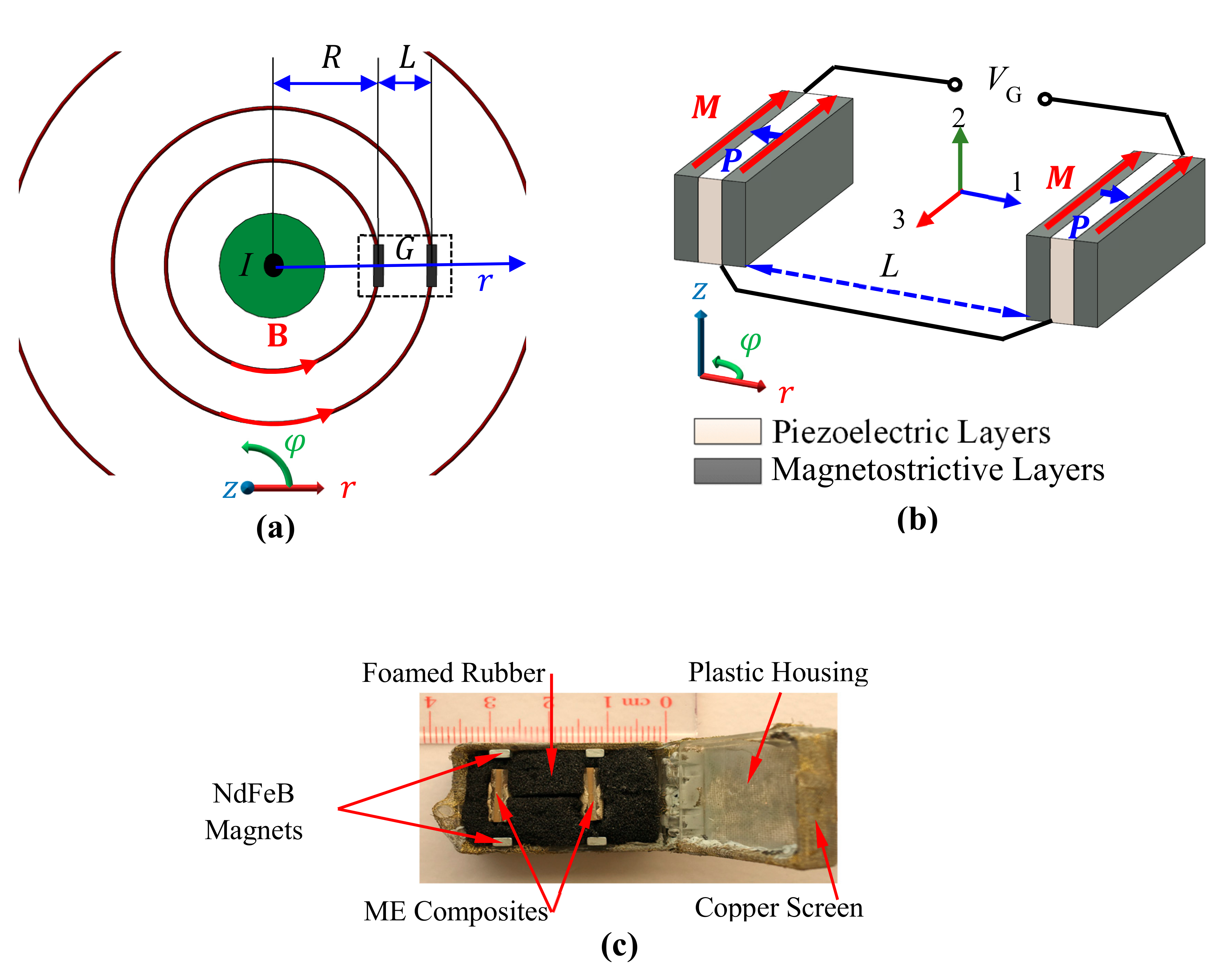
Figure 1 shows the assembly configuration, structure, and prototype of the proposed gradient-type ME current sensor. The sensor consists of a pair of plate-shaped Terfenol-D/PZT/Terfenol-D tri-layer ME composites separated with a baseline (L = 16 mm) in the radial (r-) direction, biased by two pair of NdFeB magnets () tangentially to the circumferential (-) direction, and surrounded by foamed rubber in a plastic box with copper screen shielding (see Figure 1a,b). (0.05 mm wire diameter and 0.25 mm2 hole area). The sensor is symmetrically mounted and loosely contacted with the foamed rubber in the plastic box as in Figure 1c. The usage of copper screen is to minimize the influence of ambient electric field noises based on the conductive shielding effect, and to reduce the magnetic field attenuation due to eddy current effect by reducing effective eddy current vortexes. To enable the MFG-induced ME effect for current measurement, the two ME composites are prepared by bonding a layer of PZT (Pb(Zr, Ti)O3, Ceram-Tec P8) piezoelectric ceramic plate of 12 mm length, 6 mm width, and 1 mm thickness between two layers of [112]-textured Terfenol-D (Tb0.3Dy0.7Fe1.92, Baotou Rare Earth, Baotou, China) magnetostrictive alloy plates of the same dimensions, by cutting the ME composite along its length direction (3-) using dicing saw (DAD 321, Giorgio Technology, Mesa, AZ, USA) with lowest blade feeding speed of 0.2 mm/s, blade depth of 3 mm, and by separating the obtained ME composites with dimensions of 12 mm long, 3 mm wide, and 1 mm thick. The bias magnets are made of NdFeB (N55M, V-magnet, Shanghai, China) with dimensions of 6 mm long, 3 mm wide, and 2 mm thick. As in Figure 1b, the magnetization (M) direction of the Terfenol-D plates and the polarization (P) direction of the PZT plate are oriented in their length (3-) and thickness (1-) directions, respectively. The negative electrode surfaces of the PZT plate in the two ME composites are electrically connected together to form a back-to-back capacitor configuration, while the positive electrode surfaces of the first and second PZT plates are connected to the signal core and ground shield of the coaxial cable with BNC termination, respectively. Therefore, the output voltage is directly obtained from the ME composites pair, and is directly calibrated against current amplitude to give the current sensitivity characterized by a unit output voltage per unit ampere in the cable.
3. Working Principle
3.1. Current Sensing Based on MFG Detection and Conversion
The working principle of the sensor can be described by detecting the current ()-induced MFG () and converting the detected into voltage () (i.e., MFG detection and conversion) in accordance with the product effect of the current-induced MFG effect and the MFG-induced ME effect. As shown in Figure 1a, the magnetic field strength B at the position r around a current-carrying cable is governed by:
whose gradient () is defined as the spatial differential of in the radial (-r) direction as:
When an ME gradient sensor with gradient-ME voltage coefficient () is assembled at certain position R (Figure 1a), the current-induced gradient-ME voltage () reads:
Defining the sensitivity of the gradient-type ME current sensor () as a unit voltage output per unit current, can be derived from Equations (1)–(3) as:
The right-hand side in Equation (4) demonstrates the products mechanism of current-induced MFG effect and the MFG-induced ME effect in the proposed current sensor, in which the MFG-induced ME effect is quantified by and the current-induced MFG is represented by the remaining [30]. The middle parts in Equations (4) also provide an alternative interpretation on the working principle of the sensor as an MFG-mediated ME current sensor.
Practically, the spatial differential of in Equation (4) is obtained by spatially differencing and over the baseline L in radial (r-) direction as:
By substituting Equation (5) into Equation (4), the designed of the sensor as function of assembly parameters ( and ) turns out to be
3.2. Coupling and Suppression of Multsource Noises
The output voltage from the ME composites pair can be also theoretically expressed as in Equation (7) because of the back-to-back capacitor configuration in Figure 1b.
in which and are superposition of ME voltages in each ME composites and total voltage noises ( and ) as in Equation (8).
in which in Equation (8) is the conventional ME voltage coefficients.
Figure 2 shows the multisource noise coupling mechanism in the sensor using Ishikawa diagram. In Equation (8), and are contributed by magnetic fields noise ()-induced voltage noise (), electric field noise ()-induced voltage noise (), vibration noise ()-induced voltage noise (), and thermal voltage noise () as:
in which is coupled into following the conventional ME effect as:
In Equation (9), is coupled into by means of capacitive coupling. For open-circuit condition, can be expressed as:
in which is the input resistance of external circuit, the frequency, the vaccum permitivity, the relative permittivity matrix, the normal direction vector of the electrode, the surface geometry of a positive electrode, and dS the surface element of a positive electrode.
In Equation (9), is mainly contributed by acceleration ()-induced piezoelectric voltage. The amplitude of is determined by the shape and assembly conditions of the test platform; however, a semi-empirical form of under open-circuit condition can be expressed as function of given in Equation (12).
in which is the average density of an ME composite, the thickness of piezoelectric plate, the piezoelectric the coupling matrix in stress-charge form under a constant electric field, and the fourth-order elastic matrix of the piezoelectric plate under constant static electric field [30].
In Equation (9), is temperature (T) and frequency (f)-dependent noises (thermal noises) contributed by dielectric loss noise and 1/f noise, which are written as shown by the first and second term in Equation (13), respectively.
in which , are dielectric loss factor, Boltzmann’s constant, and temperature, respectively. and are the equivalent frequency band width of measurement equipment and capacitor of the ME composite, respectively [31].
When the gradient-type ME current sensor is working in multisource noises-interfered environment to sense in a cable, voltage noises in each ME composite are essentially common-mode noises (). Therefore, the real output voltage from the sensor () can be derived by combining Equations (6)–(9) in form of the superposition of current signal part and noise part ():
in which is the suppressed total voltage noises from the current sensor written as:
To evaluate the noise suppression performance, the CMRR of gradient-type ME current sensor is defined as the ratio of the powers in over that of in unit of positive decibel as:
4. Performance Evaluation, Results, and Discussion
4.1. Intrincsic Performance
4.1.1. Evaluation of Voltage Coefficient of MFG-Induced ME Effect
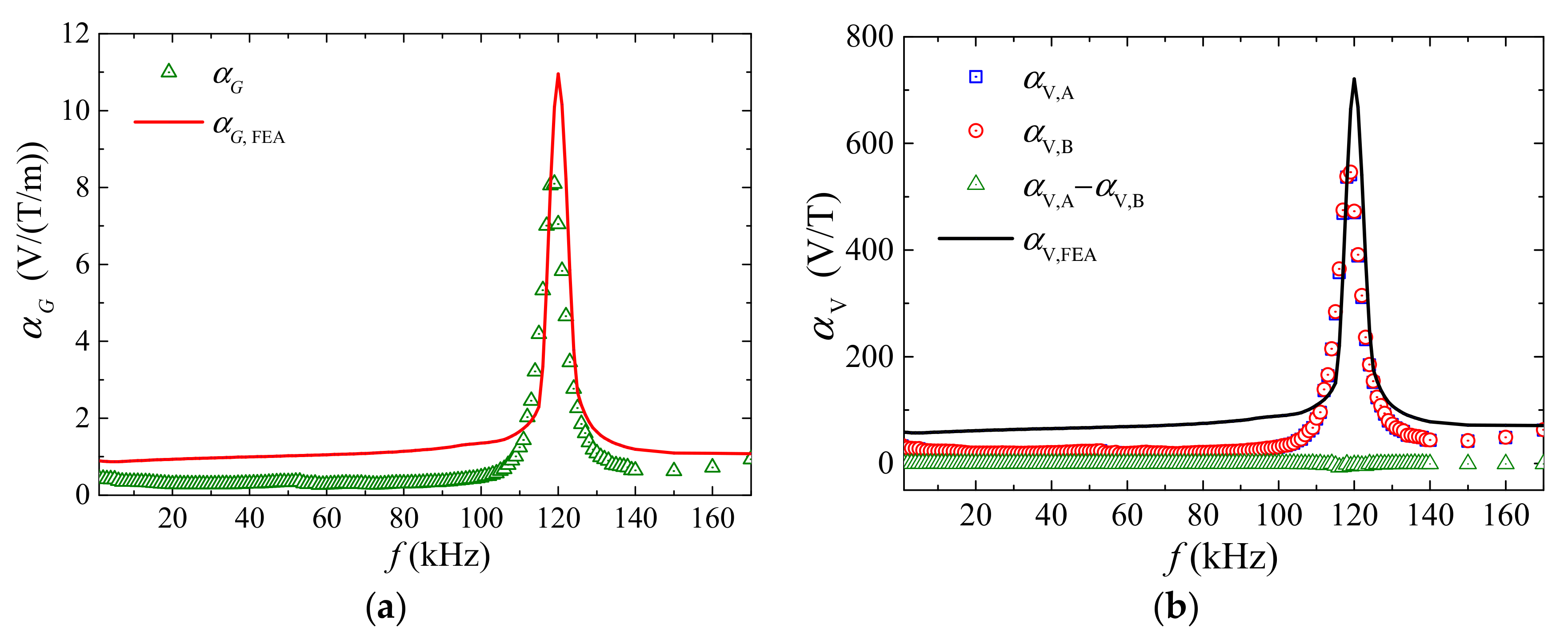
Figure 3a plots the frequency (f) dependence of the measured and calculated gradient-ME voltage coefficient ( and ) of the sensor using the methods in [30]. The and spectra are quantitatively similar to the spectra in Figure 3b, suggesting the determination of by and described by Equation (8). Non-resonance of 0.34 V/T/m is achieved over a broad frequency range of 1 Hz–80 kHz, while the highest of 8.6 V/(T/m) is obtained at resonance frequency, of 120 kHz.
Figure 3b plots the frequency (f) dependence of the measured ME voltage coefficients of the two ME composites ( and ) and their difference () for comparison with that of the ME voltage coefficient calculated from FEA () following the modeling methods in [30]. It is seen from Figure 3b that the and spectra have a difference () that fluctuates about zero in the frequency range of 1 Hz–170 kHz with relative error (/)) < 0.5%, which is one-sixth of that in [30]. This excellent similarity in the two ME composites is enabled by the improved manufacturing method described in Section 2, and well supports the condition of of the ME composites pair in the current sensor. Both and exhibit a resonance peak of ~541 V/T at the resonance frequency of 120 kHz, corresponding to a half longitudinal wavelength of 12 mm in the ME composites. Non-resonance and has an average value of 28 V/T from 1 Hz to 100 kHz.
4.1.2. Calibration of Current Sensitivity
Figure 4a shows the frequency (f) dependence of the measured current sensitivity () when R = 8 mm. The spectrum was obtained by fixing the current sensor around a straight cable (AWG-10) in the r– plane as in Figure 1a, by producing an AC reference voltage of constant amplitude over the prescribed frequency range of 1 Hz–170 kHz using a lock-in amplifier (SRS® SR865, Sunnyvale, CA, USA), by converting and amplifying the AC reference voltage into the corresponding AC current using a current supply amplifier (AE Techron® 7548, Elkhart, IN, USA), by driving the cable with the AC current of 0–20 A in steps of 0.5 A, by measuring using the lock-in amplifier, and by calculating the slope of curves at each frequency. The AC current was monitored and assured using a current probe (HIOKI® 9273, Nagano, Japan) and a signal conditioner (HIOKI® 3271) connected to the current feedback input of the lock-in amplifier. An average of non-resonance of 0.62 mV/A is achieved over a broad frequency range of 1 Hz–80 kHz, while high resonance of 8.4 mV/A is obtained at of 120 kHz. The similarity trends in Figure 3a and Figure 4a implicit a linear relationship between current-induced MFG effect and the MFG-induced ME effect as described by Equations (4) and (6).
Figure 4b shows the measured (symbols) and calculated (solid lines) and at various current amplitude of 0–20 A at 50 Hz when R = 8, 10, 12, 14, and 16 mm, respectively. Measured in Figure 4b was obtained by dividing measured over measured in Figure 3a, while calculated and were obtained using Equations (2) and (3), respectively. The difference between measured and calculated results, when R < 10 mm, can be explained by the flux distraction effects in the Terfenol-D plates when the ME composites is close to the cable. However, the straight curves in Figure 4b suggest that flux distraction effects will not affect the accuracy and input-output non-linearity of the current sensor. A very small input-output nonlinearity is evaluated to be <500 ppm in the current range of 0–20 A.
Figure 4c shows the measured (symbols) and calculated (solid lines) and at various R. was obtained using the same method as Figure 4b, while was obtained by evaluating the slopes of curves in Figure 4b. Figure 4c indicates that a maximum of 0.65 mV/A is achieved at R = 8 mm. This result suggests an optimal assembly configuration that fixing the current sensor closer to the cable center will results in higher sensitivity. The obtained sensitivity is six-times higher than that of general Hall elements current sensors and Rogowski coils.
4.1.3. Evaluation of Equivlent Current Noise Density
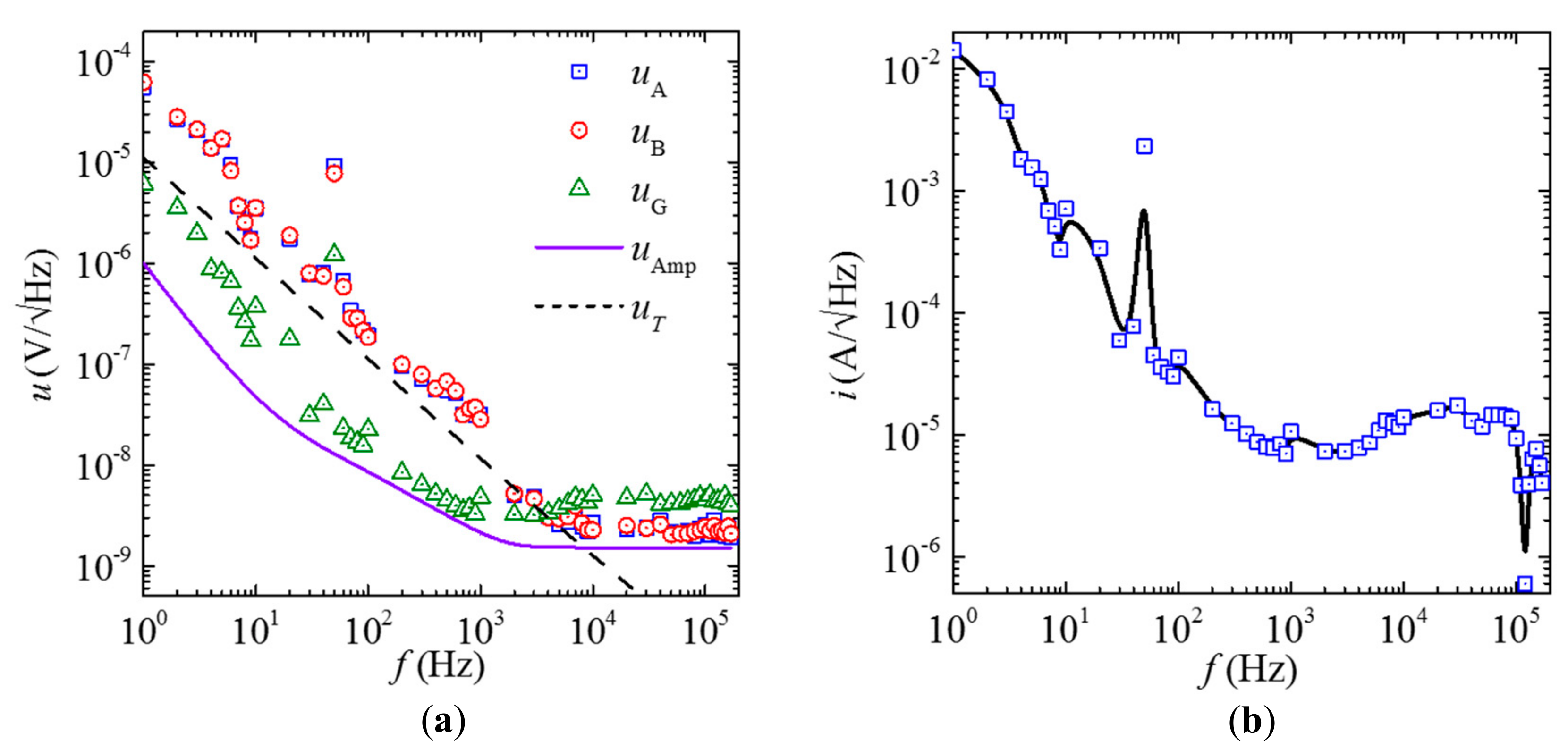
Figure 5a shows the measured voltage noise density spectra of each ME composites ( and ), the current sensor (), and the lock-in amplifier noise floor (), together with the calculated thermal noise density () spectra in a magnetically-unshielded laboratory environment at 20 °C without intentional interference. The spectra were obtained using the same method as in [30]. Since the effect of the ambient electric field noise is minimized by the copper screen shielding, the , , and spectra in Figure 5 are dominated by the thermal noises from 1 Hz to 3 kHz. In the frequency range of 20–150 Hz, the power-frequency noise arising from the magnetically-unshielded laboratory environment has an obviously added effect on . In the further elevated frequency range of 3–170 kHz, the noise associated with measurements circuit is active since , , and all fluctuate over constant values. Beyond 3 kHz, becomes double of and , which can be explained by the phase-lag between the voltage noises ( and ) in the two ME composites at high f because the voltage noises have random phases at high f (i.e., > 3 kHz).
Figure 5b shows the intrinsic equivalent current noise density (i) spectrum in a magnetically-unshielded laboratory environment at 20 °C without intentional interference. The i spectrum was evaluated using measured in Figure 5a devided by measured in Figure 4a at each frequency in a like manner to the methods in [31]. It is found that the proposed gradient-type ME current sensor has intrinsic equivalent current noise density of 0.6 A/–14.3 mA/ in the frequency range of 1 Hz–170 kHz.
4.2. Extrincsic Performance
4.2.1. Evaluation of Thermal Stability
Figure 6 shows the measured temperature (T) dependence of current measurement sensitivity (). The – curve characterized in a modified non-magnetic turbo convection oven (Fangchu®, Guangzhou, China), with two via holes on the top and bottom covers to enable the straight current carrying cable pass through the oven. By controlling the temperature slowly increase from 18 °C to 65 °C with step of 5 °C and 10 min holding time to ensure thermal equilibrium state of the system, the
at each temperature is obtained using the method described in Section 4.1.2. We see from Figure 6 that an increasing trend of
as function of T can be found within 18–65 °C. The . approximately linearly increases in the temperature range of 18–65 °C, while it decreases when T > 50 °C. The curve is in agreement with previous studies on thermal stability of ME composites, and may explained by increasing trend in temperature-dependent piezoelectric charge coefficients of PZT-8 plates and the soften effects of epoxy hardener at higher temperatures [28]. In detail, at low temperature range (18–50 °C), the rapid increasing trend of can be attributed to piezoelectric charge coefficient of PZT-8 plates. However, when temperature continues to increase (T > 50 °C), the epoxy becomes soft and consequently weakens the mechanical coupling between Terfenol-D plates and PZT-8 plates, resulting in the slow increase of as function of T. An overall relative sensitivity drift of <0.2%/°C is achieved in the temperature range of 18–65 °C.
4.2.2. Evaluation of Magnetic Fields Noise
Figure 7 shows the experiment waveforms of -induced in and , and in when the is artificially created in sine, pulse, and square waveforms, respectively. The waveforms in Figure 7 are experimentally obtained by settling a Helmholtz coil approximately 0.2 m away from the current sensor, by exciting the Helmholtz coil with a constant current supply amplifier (AE Techron® 7548, Elkhart, IN, USA) connected to an arbitrary waveform generator (Agilent® 33210A, Santa Clara, CA, USA), by monitoring the current in the coil with a current probe (HIOKI® 9273, Nagano, Japan) and it signal conditioner (HIOKI® 3271, Nagano, Japan), and by recording , , and using an oscilloscope (Tektronix® MSO2014, OR, USA). Results in Figure 7a indicate that the 50 Hz component of and are of same amplitude of 1.5 mV, while the 50 Hz component of in is 0.2 mV. The in is evaluated to be 7 times smaller than in and , corresponding to a CMRR of 17 dB in a interfered environment arising from ambient power cables. Results in Figure 7b are obtained by exciting the Helmholtz coil using pulse width-modulated current signal with pulse width of 10 , rising edge of 40 ns, and period of 20 ms in analogous to possible discharge current-induced . Waveforms in Figure 7b indicate that the peak value of and are of same amplitude of 5 mV, while the suppressed peak value of in waveforms is less than 0.2 mV. The in is evaluated to be 12 times smaller than in and , corresponding to a CMRR of 28 dB. The larger CMRR in this case can be explained by high frequency component in the pulse signal and high in Figure 3a. The zero-crossing waveforms in Figure 7b can be explained by eddy current effects and magnetostrictive effects in Terfenol-D plates. Results in Figure 7c are obtained by exciting the Helmholtz coil using square wave current signal with period of 20 ms and rising edge of 0.1 ms in analogous to possible induced by pulse-width modulated actuator in the electrical system. Results in Figure 7c have similar trends to those in Figure 7b, except for the larger transition time at the edge of square wave, which can be explained by the parasitic capacitance, eddy current effects, and magnetostrictive effects in Terfenol-D plates. The in is evaluated to be 12 times smaller than in and , corresponding to a CMRR of 21 dB.
To summarize, results in Figure 7 obviously suggest that -induced can be suppressed up to 25 times, corresponding to a CMRR up to 28 dB in the present gradient-type ME current sensor. However, it is interesting to find that the high frequency noise components of are almost 1.4 times that of , because high frequency thermal noises with random phase lag between and result in doubled .
4.2.3. Evaluation of Electric Field Noise
Figure 8 shows the experiment waveforms of -induced in and , and in when the is artificially created in sine, pulse, and square waveforms, respectively. Experiments are conducted by assembling the sensor in the middle of two home-made copper plates with separating distance of 50 mm, by applying voltage excitation to the two copper plates by voltage amplifier (AE Techron® 7548, Elkhart, IN, USA) connected to an arbitrary waveform generator (Agilent® 33210A, Santa Clara, CA, USA), and by recording , ,and using an oscilloscope (Tektronix® MSO2014, Beaverton, OR, USA). The two coppers plates both have width, length, and thickness of 100 mm, 100 mm, and 1 mm, respectively. Figure 8a shows the waveforms of , , and when the excitation voltage is sine wave with amplitude of 50 V (). Figure 8a suggest that 50 Hz components of in and amplitudes are approximately 2.1 mV, while the 50 Hz component of in is 0.18 mV. The in is evaluated to be 11 times smaller than in and , and the CMRR is evaluated to be 21 dB without the copper screen shielding. Figure 8b shows the -induced waveforms of , , and when the copper plates are driven by pulse width-modulated voltage signal with pulse width of 10 , rising edge of 40 ns, and period of 20 ms in analogous to possible, voltage-induced raising from the ON/OFF action of the electrical system. Figure 8b suggests that the peak values of in and are approximately 5 mV, while peak values of in are 0.7 mV. The in is evaluated to be 7 times smaller than . in and , and the CMRR is evaluated to be 17 dB without the copper screen shielding. Figure 8c shows the -induced waveforms of , , and when the copper plates are driven by square voltage signal at 50 Hz. Figure 8c suggests that the peak values of in and are approximately 5.8 mV, while peak values of in are 0.8 mV. The in is evaluated to be 7.2 times smaller than in and , and the CMRR is evaluated to be 17 dB without the copper screen shielding.
Detail investigation on waveforms in Figure 8 indicates that the -induced voltage noises are not completely suppressed, which may attribute to the unbalanced charge accumulation on the output electrodes of the sensor, as well as the sensor’s asymmetry assembly errors among the copper plates. However, by adding a grounded copper screen, in and are significantly reduced to give an extremely small in as shown in the bottom parts in Figure 8. For the grounded copper screen to shielded gradient-type ME current sensor, can be as 60 times smaller than that of in and in an un-shielded condition.
4.2.4. Evaluation of Vibration Noise
Figure 9 shows the experiment waveforms of -induced in and , and in . The experiment is conducted by fixing the sensor on Polytetrafluoroethylene (PTFE)-made holder clamped by non-magnetic clamps on a micro testers (Instron® 5948, Norwood, MA, USA); by controlling the head to move in triangular wave form with period of 0.64 s and amplitude of 5 mm to a square wave form of velocity with amplitude of 15.6 mm/s and period of 0.64 s, and pulsed acceleration with peak value of 18.35 with period of 0.32 s; and by recording , , and using an oscilloscope (Tektronix® MSO2014, Beaverton, OR, USA). Results in Figure 9 indicate that a pulsed with will raise in and up to 4.3 mV in conventional strength-type ME current sensor; however, in is more than 8 times reduced to 0.49 mV based on the MFG-induced ME effect in the gradient-type current sensor. The CMRR is evaluated to be 18 dB in the present case. A little difference between waveforms of and can be found in Figure 9, which may be caused by difference in mode shape asymmetry of the holder. However, it is safe to say that the CMRR will be much higher in the moving train sets of HSR system, since larger platforms vibrate more evenly, resulting in smaller acceleration difference at each ME composite.
5. Suppression of Multisource Noises
5.1. Experiment Setup
Figure 10 shows the schematics diagram of the experiment setup for multisource noise suppression performance evaluation. The experiment system (Figure 11) integrated the experiment designs in Section 4.2 to evaluate the performance of the sensor under simultaneously the interference of , , under constant temperature (T). The experiment is conducted by simultaneously generating using a Helmholtz coil driven by pulse width-modulated current with pulse width of 10 , rising edge of 40 ns, and period of 20 ms as described in Section 4.2.2, by generating square wave with amplitude of 1000 V/m as described in Section 4.2.3, by generating pulse with peak value of 6 as described in Section 4.2.4, and by exciting the cable using controlled sinewave I with amplitude of 1 A at 50 Hz as described in Section 4.1.2 at temperature of 25 maintained by the turbo convention oven described in Section 4.2.1.
5.2. Results and Discussion
Figure 12 shows the experiment waveforms of and , and , when measuring I under simultaneously interference of , , using the integrated experiment system for multisource noise suppression performance evaluation described in Section 5.1. It can be seen from Figure 12 that the and in and have peak values of 1.5 mV, ~0 mV, 1.6 mV, and 0.7 mV, while the amplitude of 50 Hz sine waveform component in is 1 mV. The is too small to be observe because of the MFG-induced ME effect in the sensor and shielding effect of the copper screen. The signal to noise ratio in is evaluated to be 0.63 without applying gradient-type ME current sensor. When applied, the amplitude of 50 Hz sine waveform component in is evaluated to be 0.8 mV. We may find that the high frequency component is doubled because of random phase lag between and ; however, this can be solved with the help of a low-pass filter. With the help of a 2-kHz low-pass FFT filter, the obtained thermal noise in is less than 0.15 mV, and the obtained signal to noise ratio is evaluated to be 5.3 in the present case. During the experiment, it is interesting to find the average level of is much stable than that of and . This can be explained by the low-frequency suppression enabled by MFG-induced ME effect in the sensor. To summarize, in the present experiment, the suppressions of are enabled by the MFG-induced ME effect, by combining MFG-induced ME effect and shielding technique, low-frequency by the MFG-induced ME effect, and high-frequency by the low-pass FFT filter. The results in Figure 12 demonstrate a strong multisource noise suppression performance in the proposed gradient-type ME current sensor, and promising applications for small current measurement with high-level interference of ambient magnetic fields noises, electric field noises, and vibration noises.
5. Conclusions
We have developed a small-scale and standalone gradient-type ME current sensor for a passive and direct converting electrical current in the power cables into electrical voltages while simultaneously suppressing common-mode ambient noise from multiple sources (including magnetic fields noises, electric field noises, vibration noises, and low frequency thermal noises). The sensor is based on the product effect of the current-induced MFG effect and the MFG-induced ME effect in a magnetic biased, an electrically-shielded and mechanically-enclosed ME composite pair. The performances of the sensor porotype are systematically characterized to achieve a high sensitivity of 0.65–12.55 mV/A in the frequency range of 10 Hz–170 kHz, a strong multisource CMRR of 17–28 dB, a small input-output nonlinearity of <500 ppm, and a small thermal drift of <0.2%/ within the measurement range of 0–20 A. The high sensitivity, strong multisource CMRR, in conjunction with the passive, direct, and broadband current detection ability in a small-scale and standalone package, enables the use of a high reliability current measuring technique for electrical condition monitoring in hash environments such as the electrical mobility system and power plants.
Acknowledgments
This work was supported in part by the Research Grants Council of the HKSAR Government under grant No. 522813, in part by the Innovation and Technology Commission of the HKSAR Government to the Hong Kong Branch of National Rail Transit Electrification and Automation Engineering Technology Research Center under grant No. 1-BBYW, and in part by the Postgraduate Studentship of The Hong Kong Polytechnic University under Project RTUY.
Author Contributions
Mingji Zhang performed both the theoretical and experimental work. Siu Wing or conceived the project and guided Mingji Zhang in the whole work.
Conflicts of Interest
The authors declare no conflict of interest.
References
- Ripka, P. Electric current sensors: A review. Meas. Sci. Technol. 2010, 21, 1–23. [Google Scholar] [CrossRef]
- Morello, R.; Mukhopadhyay, S.; Liu, Z.; Slomovitz, D.; Samantaray, S. Advances on sensing technologies for smart cities and power grids: A Review. IEEE Sens. J. 2017, 17, 7596–7610. [Google Scholar] [CrossRef]
- Xiao, C.C.; Zhao, L.Y.; Asada, T.; Odendaal, W.; Van Wyk, J. An overview of integratable current sensor technologies. In Proceedings of the 38th IAS Annual Meeting, Industry Applications Conference 2003, Salt Lake City, UT, USA, 12–16 October 2003; pp. 1251–1258. [Google Scholar]
- Shaukat, N.; Khan, B.; Ali, S.; Mehmood, C.; Khan, J.; Farid, U.; Majid, M.; Anwar, S.M.; Jawad, M.; Ullah, Z. A survey on electric vehicle transportation within smart grid system. Renew. Sustain. Energy Rev. 2017, 81, 1329–1349. [Google Scholar] [CrossRef]
- Varaiya, P. Smart cars on smart roads: Problems of control. IEEE Trans. Autom. Control 1993, 38, 195–207. [Google Scholar] [CrossRef]
- Hsi, P.H.; Chen, S.L. Electric load estimation techniques for high-speed railway (HSR) traction power systems. IEEE Trans. Veh. Technol. 2001, 50, 1260–1266. [Google Scholar]
- Ziegler, S.; Woodward, R.C.; Iu, H.H.C.; Borle, L.J. Current sensing techniques: A review. IEEE Sens. J. 2009, 9, 354–376. [Google Scholar] [CrossRef]
- Sun, X.H.; Huang, Q.; Jiang, L.J.; Pong, P.W. Overhead high-voltage transmission-line current monitoring by magnetoresistive sensors and current source reconstruction at transmission tower. IEEE Trans. Magn. 2014, 50, 1–5. [Google Scholar] [CrossRef] [Green Version]
- Leung, C.M.; Or, S.W.; Ho, S.L.; Lee, K.Y. Wireless condition monitoring of train traction systems using magnetoelectric passive current sensors. IEEE Sens. J. 2014, 14, 4305–4314. [Google Scholar] [CrossRef]
- Samimi, M.H.; Mahari, A.; Farahnakian, M.A. The Rogowski coil principles and applications: A review. IEEE Sens. J. 2015, 15, 651–658. [Google Scholar] [CrossRef]
- Ward, D.A.; Exon, J.L.T. Using Rogowski coils for transient current measurements. Eng. Sci. Educ. J. 1993, 2, 105–113. [Google Scholar] [CrossRef]
- Dupraz, J.; Fanget, A.; Grieshaber, W.; Montillet, G. Rogowski coil: Exceptional current measurement tool for almost any application. In Proceedings of the IEEE Power Engineering Society General Meeting 2007, Tampa, FL, USA, 24–28 June 2007; pp. 1–8. [Google Scholar]
- McNeill, N.; Gupta, N.K.; Burrow, S.G.; Holliday, D.; Mellor, P.H. Application of reset voltage feedback for droop minimization in the unidirectional current pulse transformer. IEEE Trans. Power Electron. 2008, 23, 591–599. [Google Scholar] [CrossRef]
- McNeill, N.; Gupta, N.K.; Armstrong, W.G. Active current transformer circuits for low distortion sensing in switched mode power converters. IEEE Trans. Power Electron. 2004, 19, 908–917. [Google Scholar] [CrossRef]
- Román, M.; Velasco, G.; Conesa, A.; Jeréz, F. Low consumption flux-gate transducer for AC and DC high-current measurement. In Proceedings of the IEEE Power Electronics Specialists Conference, Rhodes, Greece, 15–19 June 2008; pp. 535–540. [Google Scholar]
- Dezuari, O.; Belloy, E.; Gilbert, S.; Gijs, M. Printed circuit board integrated fluxgate sensor. Sens Actuators A Phys. 2000, 81, 200–203. [Google Scholar] [CrossRef]
- Lenz, J.; Edelstein, S. Magnetic sensors and their applications. IEEE Sens. J. 2006, 6, 631–649. [Google Scholar] [CrossRef]
- Open Loop Hall Effect Sensors. Available online: https://buy.fwbell.com/current-sensors/open-loop-hall-effect-sensors.html (accessed on 30 October 2017).
- Yang, X.; Li, Y.; Zheng, W.; Guo, W.; Wang, Y.; Yan, R. Design and realization of a novel compact fluxgate current sensor. IEEE Trans. Magn. 2015, 51, 1–4. [Google Scholar] [CrossRef]
- Bichurin, M.; Petrov, R.; Leontiev, V.; Semenov, G.; Sokolov, O. Magnetoelectric current sensors. Sensors 2017, 17, 1271. [Google Scholar] [CrossRef] [PubMed]
- Leung, C.M.; Or, S.W.; Zhang, S.Y.; Ho, S. Ring-type electric current sensor based on ring-shaped magnetoelectric laminate of epoxy-bonded Tb0.3Dy0.7Fe1.92 short-fiber/NdFeB magnet magnetostrictive composite and Pb(Zr,Ti)O3 piezoelectric ceramic. J. Appl. Phys. 2010, 107, 09D918. [Google Scholar] [CrossRef]
- Ramboz, J.D.; Destefan, D.E.; Stant, R.S. The verification of Rogowski coil linearity from 200 A to greater than 100 kA using ratio methods. In Proceedings of the 19th IEEE Instrumentation and Measurement Technology Conference (IMTC/2002), Anchorage, AK, USA, 21–23 May 2002; pp. 687–692. [Google Scholar]
- Tipek, A.; O’Donnell, T.; Connell, A.; McCloskey, P.; O’Mathuna, S. PCB fluxgate current sensor with saturable inductor. Sens Actuators A Phys. 2006, 132, 21–24. [Google Scholar] [CrossRef]
- Sun, C.; Wen, Y.; Li, P.; Ye, W.; Yang, J.; Qiu, J. Self-contained wireless Hall current sensor applied for two-wire zip-cords. IEEE Trans. Magn. 2016, 52, 1–4. [Google Scholar] [CrossRef]
- Zhang, J.; Li, P.; Wen, Y.; He, W.; Yang, A.; Lu, C. High-resolution current sensor utilizing nanocrystalline alloy and magnetoelectric laminate composite. Rev. Sci. Instrum. 2012, 83, 115001. [Google Scholar] [CrossRef] [PubMed]
- Eerenstein, W.; Mathur, N.; Scott, J.F. Multiferroic and magnetoelectric materials. Nature 2006, 442, 759–765. [Google Scholar] [CrossRef] [PubMed]
- Nan, C.W.; Bichurin, M.I.; Dong, S.X.; Viehland, D.; Srinivasan, G. Multiferroic magnetoelectric composites: Historical perspective, status, and future directions. J. Appl. Phys. 2008, 103. [Google Scholar] [CrossRef]
- Shen, Y.; Gao, J.; Wang, Y.; Li, J.; Viehland, D. Thermal stability of magnetoelectric sensors. Appl. Phys. Lett. 2012, 100, 173505. [Google Scholar] [CrossRef]
- Dong, S.X.; Bai, J.G.; Zhai, J.; Li, J.F.; Lu, G.Q.; Viehland, D. Circumferential-mode, quasi-ring-type, magnetoelectric laminate composite-a highly sensitive electric current and/or vortex magnetic field sensor. Appl. Phys. Lett. 2005, 86, 182506. [Google Scholar] [CrossRef]
- Zhang, M.; Or, S.W. Magnetoelectric transverse gradient sensor with high detection sensitivity and low gradient noise. Sensors 2017, 17, 2446. [Google Scholar] [CrossRef] [PubMed]
- Wang, Y.J.; Gao, J.Q.; Li, M.H.; Shen, Y.; Hasanyan, D.; Li, J.F. A review on equivalent magnetic noise of magnetoelectric laminate sensors. Philos. Trans. R. Soc. A 2014, 372. [Google Scholar] [CrossRef] [PubMed]
Figure 1.
The novel gradient-type ME current sensor based on the product effect of current-induced MFG effect and the MFG-induced ME effect: (a) top-view of current sensor assembly configuration and magnetic fields (B) and its gradient () generated in the vicinity of a current (I)-carrying cable (b) structure of ME composites pair in the sensor, in which M denotes the magnetization direction of the magnetostrictive layers and P indicates the polarization direction of the piezoelectric layer; (c) packaged prototype.

Figure 2.
Ishikawa diagram of multisource noise coupling mechanism in the proposed gradient-type ME current sensor.
Figure 2.
Ishikawa diagram of multisource noise coupling mechanism in the proposed gradient-type ME current sensor.

Figure 3.
Frequency (f) dependence of: (a) measured gradient-ME voltage coefficient and its calculated results from FEM (); (b) measured ME voltage coefficients of the two ME composites ( and ) and their difference (), together with that of the ME voltage coefficient calculated from FEA ().
Figure 3.
Frequency (f) dependence of: (a) measured gradient-ME voltage coefficient and its calculated results from FEM (); (b) measured ME voltage coefficients of the two ME composites ( and ) and their difference (), together with that of the ME voltage coefficient calculated from FEA ().

Figure 4.
(a) Frequency (f) dependence of the measured current sensitivity () when R = 8 mm, (b) measured (symbols) and calculated (solid lines) and various current amplitude at 50 Hz, and (c) measured (symbols) and calculated (solid lines) and at various R of 8–20 mm at 50 Hz.
Figure 4.
(a) Frequency (f) dependence of the measured current sensitivity () when R = 8 mm, (b) measured (symbols) and calculated (solid lines) and various current amplitude at 50 Hz, and (c) measured (symbols) and calculated (solid lines) and at various R of 8–20 mm at 50 Hz.

Figure 5.
(a) Measured voltage noise density spectra of each ME composites ( and ), the current sensor (), and the lock-in amplifier noise floor (), together with the calculated thermal noise density () spectra. (b) Measured (symbols) and fitted (solid lines) equivalent current noise density (i) spectra in a magnetically-unshielded laboratory environment at 20 °C without intentional interference.

Figure 6.
Experiment results of thermal stability: temperature (T) dependence of current measurement sensitivity ().
Figure 6.
Experiment results of thermal stability: temperature (T) dependence of current measurement sensitivity ().

Figure 7.
Experimental results of ambient magnetic field noises ()-induced voltage noises in , , and when is created by (a) sine wave, (b) pulse, and (c) square wave current excitation, respectively.
Figure 7.
Experimental results of ambient magnetic field noises ()-induced voltage noises in , , and when is created by (a) sine wave, (b) pulse, and (c) square wave current excitation, respectively.

Figure 8.
Experimental results of ambient electric field noises: ()-induced voltage noises in , , and when is created by exciting (a) sine wave, (b) pulse width modulated, and (c) square voltage signals on two copper plates, respectively. (The peak-value of is approximately 1000 V/m for all cases).
Figure 8.
Experimental results of ambient electric field noises: ()-induced voltage noises in , , and when is created by exciting (a) sine wave, (b) pulse width modulated, and (c) square voltage signals on two copper plates, respectively. (The peak-value of is approximately 1000 V/m for all cases).

Figure 9.
Experimental results of vibrational acceleration noises: ()-induced voltage noises in , , and .
Figure 9.
Experimental results of vibrational acceleration noises: ()-induced voltage noises in , , and .

Figure 10.
Schematics diagram of experiment setup for multisource noise suppression performance evaluation. Labels, lines, and arrows with colors of magenta, brown, blue, green, and red represent -, -, -, , and T-related equipments, respectively.
Figure 10.
Schematics diagram of experiment setup for multisource noise suppression performance evaluation. Labels, lines, and arrows with colors of magenta, brown, blue, green, and red represent -, -, -, , and T-related equipments, respectively.
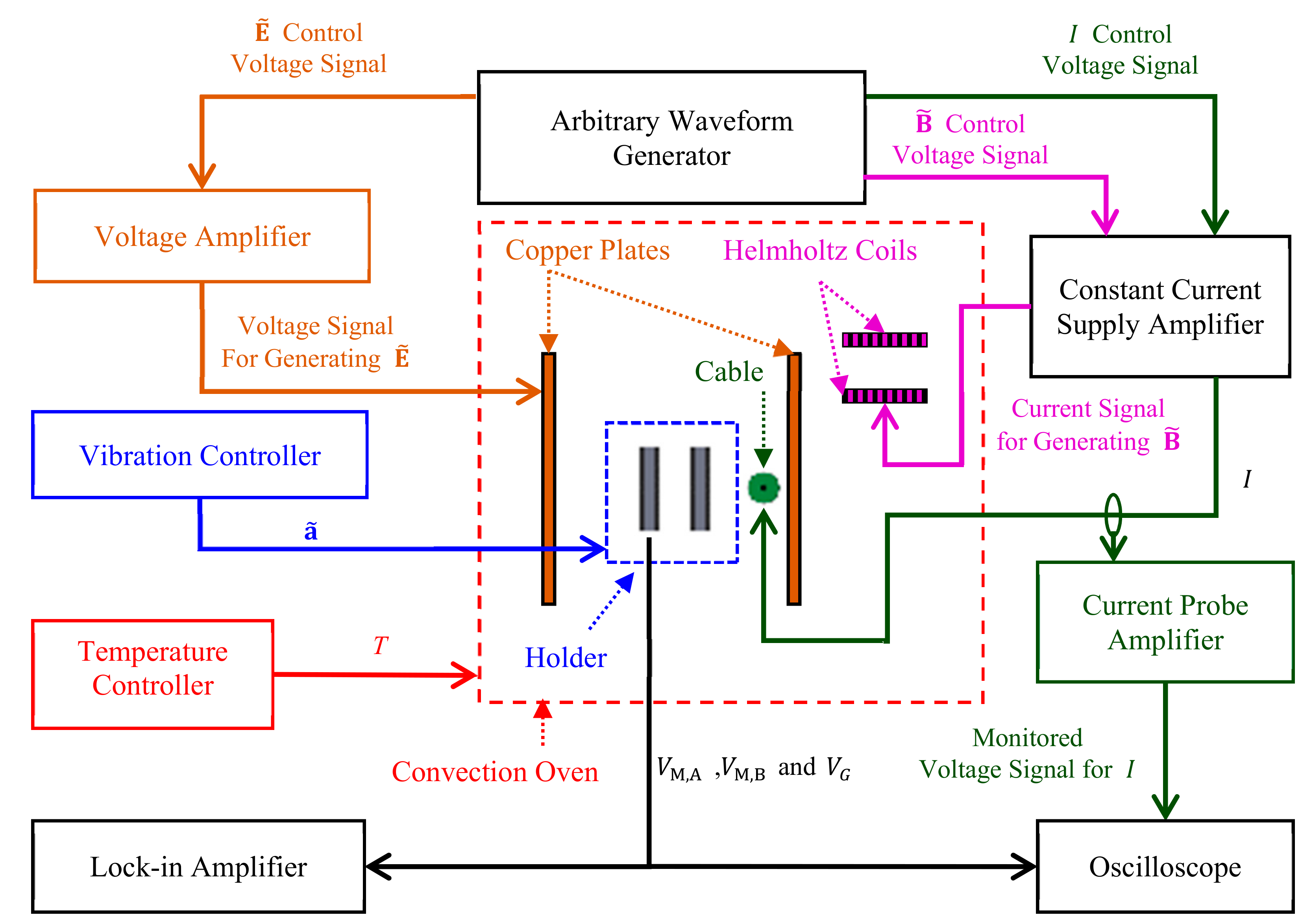
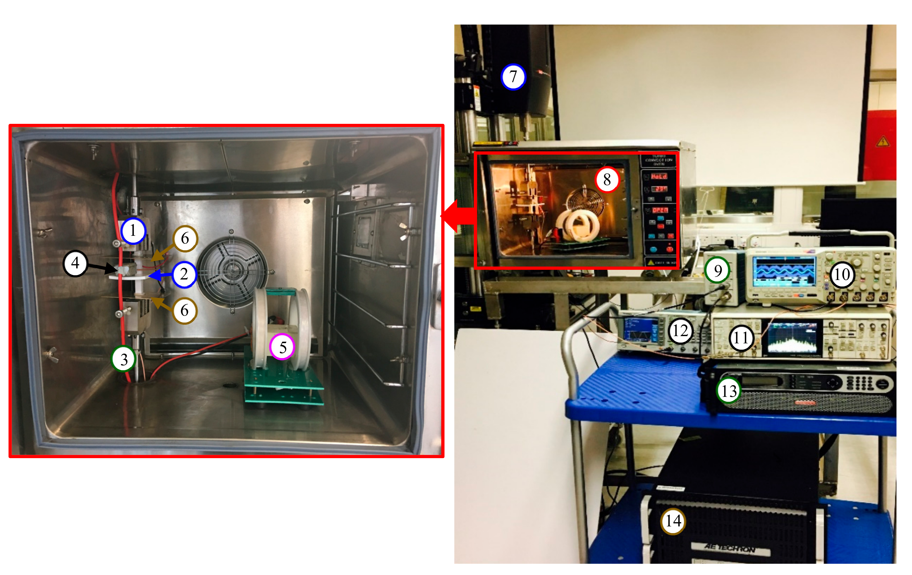
Figure 11.
Experiment system for multisource noise suppression performance evaluation. Labels with colors of magenta, brown, blue, green, and red represent -, -, -, -, and T-related equipment, respectively. (1. Vibration head; 2. Holder; 3. Cable; 4. Sensor; 5. Helmholtz coils; 6. Copper plates; 7. Vibration controller; 8. Convection oven; 9. Current probe amplifier; 10. Oscilloscope; 11. Lock-in amplifier; 12. Arbitrary waveform generator; 13. Constant-current supply amplifier; 14. Constant-voltage amplifier).

Figure 12.
Experiment waveforms of and , and , (green for raw data waveform, and black for 2-kHz low-pass filtered waveform) when measuring I in the cable under simultaneously interference of , , , and thermal noises.
Figure 12.
Experiment waveforms of and , and , (green for raw data waveform, and black for 2-kHz low-pass filtered waveform) when measuring I in the cable under simultaneously interference of , , , and thermal noises.

© 2018 by the authors. Licensee MDPI, Basel, Switzerland. This article is an open access article distributed under the terms and conditions of the Creative Commons Attribution (CC BY) license (http://creativecommons.org/licenses/by/4.0/).
Share and Cite
MDPI and ACS Style
Zhang, M.; Or, S.W. Gradient-Type Magnetoelectric Current Sensor with Strong Multisource Noise Suppression. Sensors 2018, 18, 588. https://doi.org/10.3390/s18020588
AMA Style
Zhang M, Or SW. Gradient-Type Magnetoelectric Current Sensor with Strong Multisource Noise Suppression. Sensors. 2018; 18(2):588. https://doi.org/10.3390/s18020588
Chicago/Turabian StyleZhang, Mingji, and Siu Wing Or. 2018. "Gradient-Type Magnetoelectric Current Sensor with Strong Multisource Noise Suppression" Sensors 18, no. 2: 588. https://doi.org/10.3390/s18020588
Note that from the first issue of 2016, this journal uses article numbers instead of page numbers. See further details here.