A Spectral Reconstruction Algorithm of Miniature Spectrometer Based on Sparse Optimization and Dictionary Learning


1
Department of Electronic Engineering, Tsinghua University, Beijing 100084, China
2
Tsinghua-Berkeley Shenzhen Institute, Tsinghua University, Shenzhen 518055, China
*
Author to whom correspondence should be addressed.
Sensors 2018, 18(2), 644; https://doi.org/10.3390/s18020644
Submission received: 5 January 2018
/
Revised: 29 January 2018
/
Accepted: 13 February 2018
/
Published: 22 February 2018
(This article belongs to the Special Issue Spectroscopy Based Sensors)
Abstract
:The miniaturization of spectrometer can broaden the application area of spectrometry, which has huge academic and industrial value. Among various miniaturization approaches, filter-based miniaturization is a promising implementation by utilizing broadband filters with distinct transmission functions. Mathematically, filter-based spectral reconstruction can be modeled as solving a system of linear equations. In this paper, we propose an algorithm of spectral reconstruction based on sparse optimization and dictionary learning. To verify the feasibility of the reconstruction algorithm, we design and implement a simple prototype of a filter-based miniature spectrometer. The experimental results demonstrate that sparse optimization is well applicable to spectral reconstruction whether the spectra are directly sparse or not. As for the non-directly sparse spectra, their sparsity can be enhanced by dictionary learning. In conclusion, the proposed approach has a bright application prospect in fabricating a practical miniature spectrometer.
1. Introduction
Spectral analysis is an elementary and indispensable approach to the qualitative and quantitative analysis of chemical materials. Thus, the spectrometer is widely used in numerous applications such as environmental monitoring, medical treatment and so on [1,2]. However, due to the equipment having sophisticated diffractive or interferometric devices such as a grating or prism, the conventional spectrometer is commonly bulky and expensive. Therefore, miniaturization of the spectrometer is a burgeoning research hotspot in both industry and academia [1,2,3,4,5,6,7,8,9,10,11,12,13,14,15,16,17,18,19,20,21]. The current commercial miniature spectrometer still utilizes a grating as its core dispersive component through the technology of micro-opto-electro-mechanical-systems (MOEMS) [3,4]. In order to reduce the size and cost of the spectrometer, various computational miniature spectrometers have been proposed and designed, in which the novel dispersive elements are employed to replace the grating [5,6,7,8,9,10,11,12,13,14,15,16,17,18,19,20,21]. For instance, photo crystal [5], linear variable optical filter [6], disordered photonic chip [7], dispersive hole array [8,9], micro interferometer array [10], liquid crystal phase retarder [11], multimode fiber [12,13], silicon multimode waveguide [14], broadband filter array [15,16,17,18,19,20] and so on are developed as the dispersive elements. Among these various miniaturization technologies, the filter-based approach shows great potential in reducing the size as well as the cost of a spectrometer, which can consequently enhance the portability and broaden the application area of spectrometry [15,16,17,18,19,20].
In the computational spectrometer, spectral reconstruction is usually modeled as solving a system of liner equations. As a result, it is necessary to use optimization algorithms to reconstruct the spectra in the computational spectrometer, which differs from the traditional direct-reading spectrometer significantly [5,6,7,8,9,10,11,12,13,14,15,16,17,18,19,20,21]. There have been several reconstruction algorithms adopted in previous studies, mainly including nonnegative least squares [5,17], least mean squares [6], simulated annealing [7,12], Tikhonov regularization [8,10,18], truncated singular value decomposition [12], direct-binary-search [21] and sparse optimization [11,13,19,20]. Several studies have demonstrated that sparse optimization performs better in terms of the reconstruction accuracy and the number of measurements [11,13,19,20].
Figure 1 presents the schematic of the filter-based miniature spectrometer. After transmitting through the filters with distinct transmission functions, the incident light is then measured by the array of photodetectors. Then the spectrum can be reconstructed from the output of the photodetector.
Ideally, the transmission functions are with a very narrow passband or similar to the delta function. Besides, different filters correspond to the specific and non-overlapping passbands, all of which jointly cover the entire operating band. In this case, the spectrum can be directly read out from the output of the photodetector, in the same way as the grating-based spectrometer. This method can be referred to as narrowband filtering. Nevertheless, it is very impractical to fabricate these ideal narrowband filters considering the craftsmanship and cost. Instead, most filters actually own the non-ideal optical filtering characteristics owing to the low-cost fabrication of broadband filters [17,18,19,20]. To be specific, their transmission functions have wide or even multiple passbands. Correspondingly, the non-ideal approach can be called broadband filtering. Unlike narrowband filtering, the detection value of broadband filtering is no longer the measured spectrum itself. Therefore, the raw spectrum needs to be reconstructed by certain signal processing algorithms [17,18,19,20].
Mathematically, spectral reconstruction is essentially solving a system of linear equations, where the number of equations equals that of the filters [17,18,19,20]. Given the measurement error or system noise, the system of linear equations usually needs to be overdetermined, which can be solved through the classical least squares (LS) algorithm [17,18]. Unfortunately, even when modified LS algorithms are adopted such as the nonnegative LS or Tikhonov regularized LS, reconstruction results often deviate from the true spectra owing to the ill-condition of the equations [18]. In addition, the spectral resolution is limited by the number of filters in this overdetermined setup, which implies more filters are needed to improve the resolution [17,18,19,20]. Hence, it is necessary to use advanced algorithms to reconstruct the spectra [19,20].
According to several recent studies, sparse optimization can improve reconstruction accuracy and at the same time decrease the number of needed filters [19,20]. As for the specific problem of spectral reconstruction, sparse optimization refers in particular to settling the l1-norm minimization problem, which is commonly used to solve the underdetermined system of equations [22,23,24,25]. In other words, the number of filters can be smaller than the dimensionality of the measured spectrum, which results in reducing the size and cost of the spectrometer further. However, sparse optimization highly demands the sparsity of reconstructed spectra. In general, the sparsity means that there are only a small number of nonzero components in the signal [22,23,24]. While there exist some kinds of directly sparse spectra, the vast majority of spectra are non-directly sparse and need to be represented in another transform domain.
Many natural signals are sparse in a certain transform domain [19,20], which is referred to as the dictionary in this paper. For example, an image signal has sparse representation coefficients in wavelet transformation [24,26]. Likewise, the spectra may be sparse in a certain dictionary, which needs to be discovered. Some researchers have used Gaussian kernels, Lorentzian and Secant Hyperbolic as the spectral dictionary, whose performances need to be further improved [19,20]. In the image processing, dictionary learning is an emerging method to train out the transform domain [27,28,29,30]. Inspired by this methodology, we adopt dictionary learning in this work to obtain the dictionary specific to the spectra.
In this paper, we propose an algorithm of spectral reconstruction based on sparse optimization and dictionary learning. To verify the effectiveness of the reconstruction algorithm, we design and implement a simple prototype of filter-based miniature spectrometer. The experimental results demonstrate that the l1-norm minimization is not only valid for the directly sparse spectra, but also effective for the general spectra that need transforming in the dictionary, indicating that dictionary learning can largely enhance the sparsity of general spectra.
The rest of this paper is organized as follows. Section 2 presents the prototype of the filter-based miniature spectrometer, including the mathematical model and the experimental implementation. Section 3 details the proposed spectral reconstruction algorithm. Section 4 demonstrates experimental results for the algorithm verification. Finally, discussions and conclusions are provided in Section 5.
2. Modeling and Implementation of the Prototype
In this section, we aim at modeling the prototype of the filter-based miniature spectrometer and then introduce the implementation of it.
2.1. System Model and Problem Formulation
As shown in Figure 1, we denote the spectrum of incident light as f(λ), a continuous function with respect to the wavelength λ. Then let represent the transmittance of the ith filter, which is measured by the standard commercial spectrometer, and m stands for the number of filters. Moreover, means the response function of the photodetector. According to the schematic, the light spectrum is modulated respectively by different transmission functions at first and then is measured by the photodetector, the output of which is denoted as the intensity . Based on this principle, the intensity is given by
where represents the measurement error [17,18,19,20]. For convenience, the spectrum to be measured can be compactly denoted as the product hereafter. Therefore, the intensity is the projection of onto the transmittance
Since the transmittance obtained by the spectrometer can only be in the discrete form, we can approximately convert the above integral to a system of linear equations:
where the intensity vector is the output of the photodetector; the sensing matrix is denoted as , where is the uniform sampling of and n is the dimensionality of the measured spectrum; is the discrete form of ; is the error vector corresponding to the measurement of different filters. Equation (2) is a classic inverse problem [12], and can be expanded into a more specific form:
As mentioned earlier, in narrowband filtering, the output of the photodetector is just the discrete sampling of the spectrum , i.e., . Namely, is the identity matrix or diagonal matrix with m = n. In this case, the number of filters is a key factor of limiting the spectral resolution, which implies more filters are needed to improve the resolution.
In broadband filtering, it is necessary to adopt the optimization algorithms to solve the inverse problem (2). More precisely, there exist two situations whether m is larger than n or not. Under the condition of m > n, the LS algorithm is commonly used to solve the overdetermined system [17,18]. It is yet regrettable that reconstruction results of LS are usually unsatisfactory even though m is much greater than n. Thus, what we are actually concerned about in this paper is the underdetermined case of m < n. In this underdetermined setup, sparse optimization works very well, and will be introduced in Section 3. Furthermore, since the number of filters can be smaller than the dimensionality of spectrum, the spectral resolution will not be limited by the number of filters any more. In this way, the size and cost of the filter-based spectrometer can be reduced further.
2.2. Design and Implementation of the Prototype
According to Figure 1, we can design a two-dimensional filter array with distinct transmittance in different places, and then couple it to the planar photodetector array such as the charge-coupled device (CCD). With this snapshot method, we can simultaneously measure all the intensities of photodetector array, which is an efficient implementation of the filter-based spectrometer [17,18,19,20]. However, this methodology requires that the incident light should uniformly distribute on the filter array. Worse still, combining the filter array together with the photodetector will easily damage the latter during the phase of experimental verification.
To circumvent the above issues, we simplify the experimental method. Instead of fabricating the filter array, we put the filters one by one in front of the photodetector to obtain the light intensity values. The prototype demonstrated in this work is simple but effective enough to show the validity of proposed algorithm.
As for the specific experimental procedure, we first preheat the light source and the photodetector to stabilize the illumination intensity and the background noise. Then we put a filter in front of the photodetector and measure the intensity many times to obtain the average value . Afterwards, put another filter and repeat the above procedure. After obtaining the intensity vector b, we can implement the proposed algorithm to reconstruct the spectrum. The experimental optical system is shown in Figure 2.
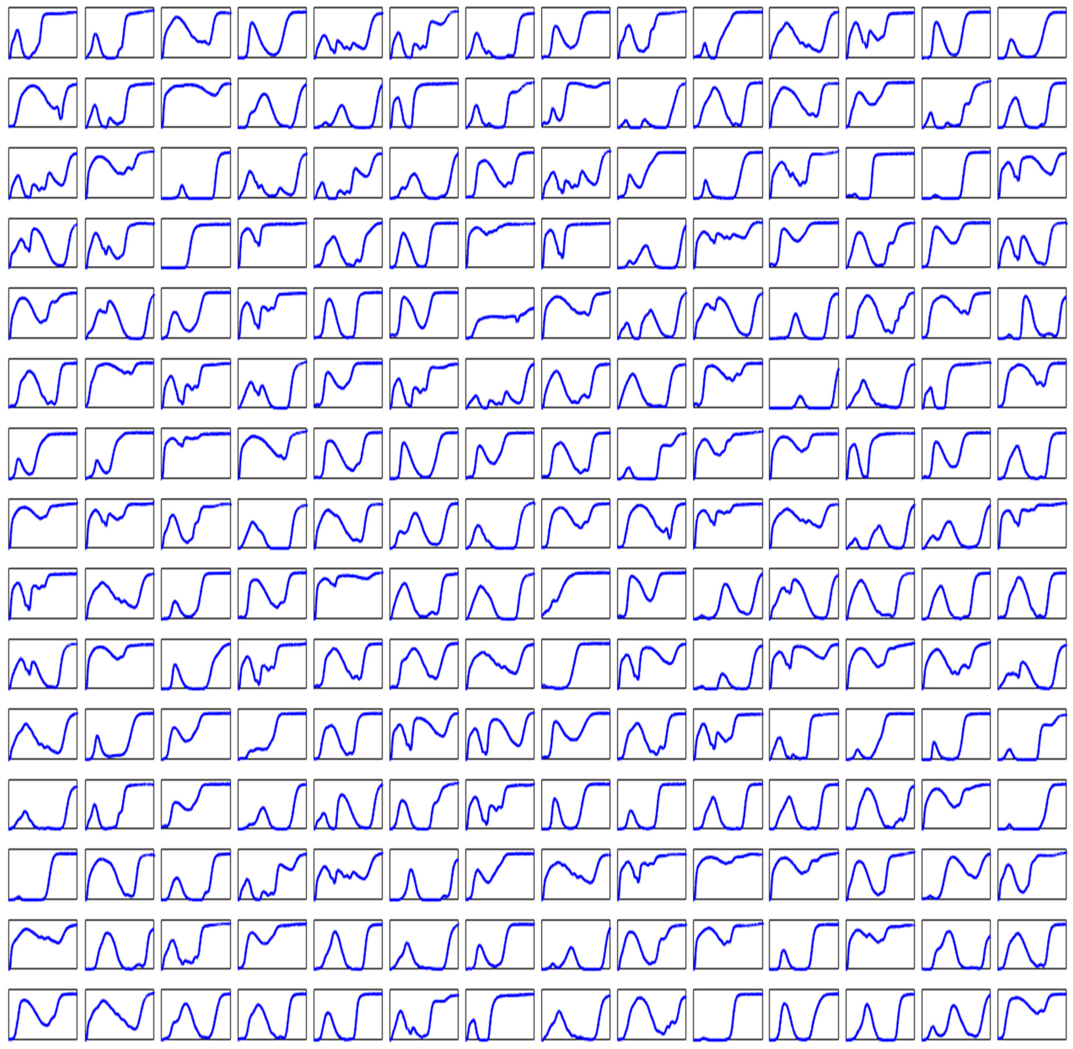
In this work, 210 filters with various colors are used during the experiments. In addition the transmission functions of them, which are all depicted in Appendix A, are measured by the commercial spectrometer with the sampling interval of 0.5 nm. Besides, in the experimental optical system we use a cut-off filter to acquire our concerned visible band. The transmission functions of some filters and the cut-off filter are displayed in Figure 3.
Moreover, it is a potential realization of hyperspectral imaging that we combine the methods of Figure 1 and Figure 2 together. To be specific, we can just put a rotational filter array in front of the photodetector of a camera and then take snapshots of a stationary object with the rotation of the filter array. Using the reconstruction algorithm proposed in this work, we may design a practical imaging spectrometer with small size and low cost in our future work.
3. Proposed Algorithm of Spectral Reconstruction
The above contents have comprehensively introduced the mathematical model and implementation details of the prototype. In this section, we elaborate on the specific algorithm of spectral reconstruction based on sparse optimization and dictionary learning.
3.1. Sparse Optimization
The advanced sparse optimization is well suitable for solving the noise-corrupted underdetermined system of linear equations [22,23,31]. In order to solve (2), we can simply optimize the following l0-norm minimization problem on condition that the spectrum is sparse:
where l0-norm is the number of nonzero elements of , and l2-norm is the Euclidean norm. Besides is a positive constant representing the noise level.
However, the l0-norm minimization (4) is a NP-hard problem [22,23,31], which is typically replaced by the following convex form,
where l1-norm is defined as . Some other versions of the l1-norm minimization to solve (2) are given in Appendix B. Herein, only if the spectrum is sparse can we get a good approximate solution of (2) by solving (5). For example, the narrowband spectra are directly sparse.
In practice, however, numerous spectra are not directly sparse in nature. Therefore, we need to transform the non-directly sparse spectrum into another domain to have its sparse representation , i.e., where is a sparse vector [22,23,31]. Consequently, the original optimization problem of (5) is converted to the following form,
After obtaining the optimal solution of (6), we can calculate the measured spectrum by where is the reconstruction of the raw spectrum by sparse optimization.
3.2. Dictionary Learning
As for the non-directly sparse spectra, how to find or design a proper transform domain is still a problem to be solved. Some studies have used Gaussian kernels, Lorentzian and Secant Hyperbolic as the transform domain, which can preserve the smooth property of spectra [19,20]. Nevertheless, these approaches are tentative and not generally applicable.
In the image processing, the dictionary learning is an emerging method to train out the transform domain [27,28,29,30], which is referred to as the dictionary in this paper. Inspired by this methodology, we adopt dictionary learning in this work to obtain the spectral dictionary, which can enhance the sparsity of general spectra and then reinforce the robustness to noise. Several related studies have detailed the training process [26,27,28,29,30]. To be specific, we collect lots of spectra as the training set , in which is a spectrum. Then we use dictionary learning to train out the dictionary such that , where is the sparse representation matrix. Each column of is called an atom, and each column of is the sparse vector representing the corresponding column of in the dictionary Herein n is the dimensionality of the spectrum, p is the total number of the spectra to be trained and k is the number of atoms.
Mathematically, dictionary learning can be formulated as the following optimization problem,
where the square of Frobenius norm is defined as for the matrix A, and is the sparse constraint on of the representation matrix . There are several well-studied dictionary learning algorithms including K-SVD [27], ILS-DLA [28], RLS-DLA [29], etc. Typically, dictionary learning needs to iteratively solve the two following problems, namely the sparse approximation and dictionary update.
- Sparse Approximation Stage: keep the dictionary fixed, and then use sparse optimization above to calculate the sparse representation of in the dictionary . That is to say, solve the inverse problem by sparse optimization;
In our work, to obtain the training set , we collect the transmittance of many variant chemicals in [32]. Besides, it is necessary to preprocess these spectra to make their sampling interval the same as the transmittance of the filters, i.e., 0.5 nm. In addition, the transmission functions of 210 filters are used as a part of the training set. To further increase the number of spectra to be trained, we multiply two arbitrary spectra of filters to have a new one. The physical meaning of the product is the transmittance obtained when we overlap the two filters together. At the last, the total number of the spectra to be trained is 3000, i.e., p = 3000.
It is noteworthy that all aforementioned spectra of the training set are the transmission functions, which do not contain the spectral information of the light source at all. Conventionally, the spectrometer has a fixed light source with the energy spectrum of a particular shape, such as the halogen lamp. The spectral information of light source will be embedded into the detection value of the spectrometer during the measurement. In other words, the spectrum to be measured is just a modulation of the source spectrum. Hence, we need to multiply the training set of transmission functions by the spectrum of the used light source, which can be measured by the spectrometer in advance.
What is more, it should be noted that the natural optical spectra are inherently non-negative. Thus, we use the non-negative dictionary learning algorithm, which means each atom of the dictionary is a non-negative vector. Herein, the solver of non-negative K-SVD is a good option to train the non-negative dictionary [33]. Likewise, in order to reconstruct the spectra successfully, the non-negative constraint should be also added to the above formulation of sparse optimization, namely (5) and (6).
In conclusion, for the directly sparse spectra, we optimize the following problem,
4. Results
All of the experimental results demonstrated in this section are mainly to show the feasibility and potential practicality of the prototype qualitatively. Based on these results, it can be concluded that not only does sparse optimization work well for the directly sparse spectra, but it also achieves the impressive performance when used to reconstruct the non-directly sparse spectra with dictionary learning. Furthermore, dictionary learning performs better than Gaussian kernels, which are used as the transform domain in several previous studies [19,20].
The main experimental instruments used in this work include a CCD camera (acA1600-20 um, Basler ace, Ahrensburg, Germany), a scientific grade spectrometer (PG2000 pro, Ideaoptics, Shanghai, China), an ultraviolet spectrophotometer (UV-2450, SHIMADZU, Kyoto, Japan), a halogen light source (HL-2000, Ocean Optics, Largo, FL, USA) and a light-emitting diode (LED) lamp.
4.1. Directly Sparse Spectra
In this subsection, we aim to evaluate reconstruction quality of the continuous narrowband spectra, which are directly sparse spectra. For reconstruction of directly sparse spectra, we need to solve the l1-norm minimization problem (8).
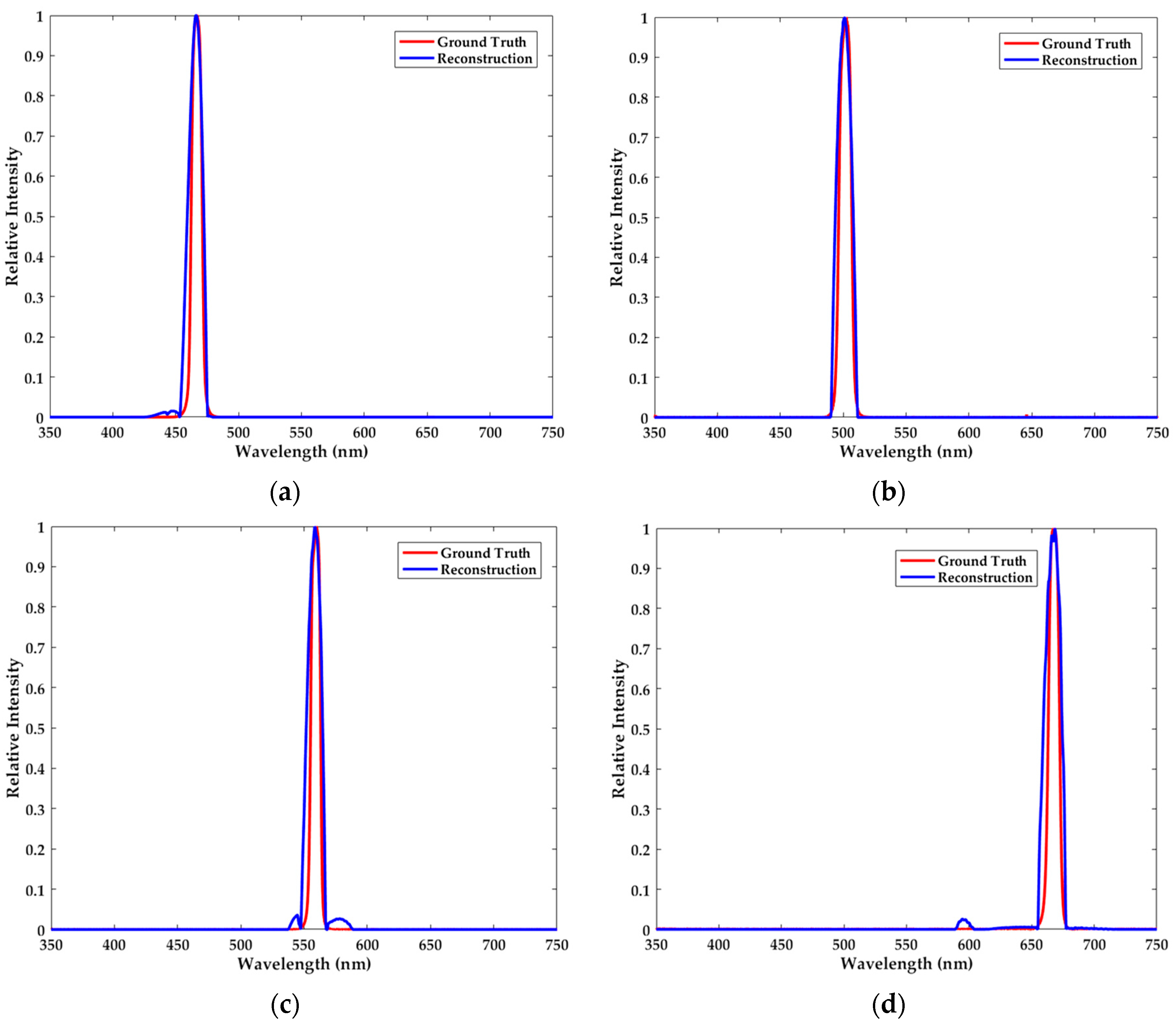
In this part of the experiment, we use four kinds of narrowband filters with the crest centering at 466.5 nm, 501.5 nm, 558.5 nm and 668.5 nm. Besides, their full width at half maximum (FWHM) is respectively 9 nm, 14 nm, 8 nm and 9 nm. As depicted in Figure 4, reconstruction results of the narrowband spectra are very satisfactory. It is noteworthy that there exist some slight perturbations in the neighborhood of the passband. Despite the reconstructed waveforms not completely coinciding with the ground truth spectra owing to the measurement error, the locations of the passband and crest can be accurately determined.
4.2. Non-Directly Sparse Spectra
Reconstruction results of non-directly sparse spectra are demonstrated in this subsection. For reconstruction of non-directly sparse spectra, we need to first adopt dictionary learning to train out the dictionary and then use the existing sparse optimization solver to solve the l1-norm minimization problem (9).
4.2.1. Halogen Lamp as the Source
Since the halogen lamp has excellent stability and strong illumination, it is commonly used as the light source of the visible-light spectrometer in spite of its high price. To obtain the dictionary specific to the halogen lamp, we need to multiply the training set of transmission functions by the spectrum of the lamp at first and then train out the dictionary using dictionary learning. In the experiments, we first reconstruct the spectrum of the halogen lamp. Afterwards, we combine three different filters respectively together with the halogen lamp as testing samples, which are measured one after another. In this part the number of filters m is 210 and the operating band is from 350 nm to 700 nm with a sampling interval of 0.5 nm, i.e., n = 701.
The results of the aforementioned experiments are listed in Figure 5. Although reconstructed spectra are somewhat discrepant from the ground truth, they share the consistent variation tendency and are similar shape as shown in Figure 5. To be specific, the crests and troughs are mostly located at the same wavelengths.
4.2.2. Light-Emitting Diode as the Source
In this part of the experiment, we use a light-emitting diode (LED) as the light source. The number of used filters m is 210 and the operating band is from 410 nm to 670 nm with the sampling interval of 0.5 nm, i.e., n = 521. In general, compared to the halogen lamp, the LED is less frequently used as the light source of the commercial spectrometer. Its energy distribution along the wavelength is non-uniform. However, in our filter-based spectrometer what we need to measure is not the individual intensity at a particular wavelength but the total intensity over the spectral band. The experiments herein, whose results are displayed in Figure 6, are performed just through the same procedures as stated in the previous part.
Likewise, the conclusions of the LED resemble those of the halogen lamp. In short, the minor deviation and the similar variation tendency coexist in the results. According to the satisfactory results, the LED may substitute the frequently used halogen lamp as the light source of the spectrometer. Consequently, the cost of the spectrometer can be further reduced by the use of inexpensive LED.
4.3. Comparison between Dictionary Learning and Gaussian Kernels
In this paper, we demonstrate a prototype combining sparse optimization with dictionary learning to reconstruct the spectra. Several previous studies have used Gaussian kernels as the transform domain of spectra [19,20]. Therefore, in this subsection we compare the performance of dictionary learning and Gaussian kernels in spectral reconstruction.
We carry out the experiments respectively on spectral reconstruction of the halogen lamp and the LED. There are two main parameters that can be adjusted in the method of Gaussian kernels, namely the mean value and standard deviation. In this comparison, we let the mean value traverse in the whole operating band with the interval of 0.5 nm. Besides, we set the standard deviation of the halogen lamp and the LED to 42 and 18 respectively. These parameters have been optimized by the brute-force search. To compare reconstruction quantitatively, we calculate the relative reconstruction error re as follows [13],
where is the raw spectrum and is the reconstructed spectrum of .
Relative reconstruction errors of dictionary learning and Gaussian kernels are respectively 5.92% and 21.09% in Figure 7a. Besides, for reconstruction of LED, the relative errors are 10.25% and 57.53% in Figure 7b. Based on these relative errors, dictionary learning performs better than Gaussian kernels. As depicted in Figure 7, the results of Gaussian kernels severely deviate from the ground truth. Worse still, it is so hard and tentative to adjust the parameters that Gaussian kernels cannot be applied in the actual spectral reconstruction. Even though we increase the number of kernels with multiple variances, there is no further improvement of reconstruction quality. While the method of Gaussian kernels can preserve the smooth feature of the spectra, it cannot capture the variation details and has little robustness to the measurement error in the experiments. According to these results, we can conclude that dictionary learning indeed contributes to finding the sparse representation of the spectra, and is beneficial for obtaining better reconstruction results when combined with sparse optimization.
4.4. Further Exploration
As previously mentioned, the l1-norm minimization is adopted to solve the underdetermined system of linear equations, in which the number of filters is far smaller than the dimensionality of spectrum. The fewer the filters are, the more simply the miniature spectrometer is fabricated. Besides, the total cost will be lowered further. Herein we explore the effect of the number of filters on reconstruction quality. As shown in Figure 8, reconstruction results are even slightly improved when we bring the number of filters down from 210 to 20, which is seemingly unaccountable but in fact reasonable.
In order to explain the results, the principle component analysis (PCA) is adopted to validate the sparsity of the spectra [38,39,40,41]. Specifically, PCA is carried out on the training set of the halogen lamp. The dimension of the spectra in the training set is 701, i.e., n = 701. Figure 9a plots all the eigenvalues of PCA in descending order, and the ten largest eigenvalues are shown in Figure 9b. Based on the theory of PCA, these rapidly descending eigenvalues visually indicate that the information contained in the spectra is very sparse, which is the necessary precondition of sparse optimization. Besides, according to Section 4.3, dictionary learning indeed largely enhances the sparsity of spectra and further makes the spectral reconstruction more robust to noise. Based on these facts, 20 proper filters actually may capture the vast majority of the spectral information. In addition, more filters will bring about more noises in our simplified method. For these reasons, when we bring the number of filters down from 210 to 20, it is possible to obtain better reconstruction results.
However, it should be clearly stated here that not every twenty filters out of the 210 could succeed in reconstructing the spectra as in Figure 8. That is to say, one group of 20 filters may get better reconstruction result, while the result of another group may be worse. Based on these findings, it can be inferred that fewer filters may put forward more stringent requirements on the property of the transmittance matrix, which will be further studied in future work.
5. Discussion and Conclusions
Among various miniaturization technologies, the filter-based spectrometer is a promising implementation, in which the inexpensive broadband filters replace the sophisticated diffractive or interferometric optical devices used in the traditional spectrometer, such as the grating or prism. The consequent problem is how to design the proper reconstruction algorithm due to the non-ideal filters. In this paper, the spectral reconstruction is accomplished by sparse optimization and dictionary learning, which can minimize the number of filters. The results demonstrate that sparse optimization applies well to the spectral reconstruction whether the spectra are directly sparse or not. For the non-directly sparse spectra, their sparse representation is obtained by dictionary learning, which outperforms the method of Gaussian kernels even with the optimized parameters by brute-force searching. In addition, according to the reconstruction quality of LED, it may be an alternative source in the filter-based spectrometer. In conclusion, everything mentioned above contribute to reducing the size and cost of the spectrometer. The approach proposed in this paper has a bright application prospect in fabricating the practical miniature spectrometer.
Our future work is mainly focused on improving the algorithm and designing the compact hardware. Since the reconstruction results above are still slightly discrepant from the true spectra, it is quite necessary to modify the algorithm used in this paper. Moreover, it is necessary to find out the relationship between the number of filters and the needed properties of the transmission functions. As regards the hardware implementation, we try to design a compact and portable miniature spectrometer with a proper filter array attached to the photodetector [16,17,18,19,20]. It is undeniable that this is an applicable and efficient method of miniaturizing the spectrometer. Furthermore, we also attempt to implement an imaging spectrometer using a rotational filter array.
Acknowledgments
This work is supported by Shenzhen Engineering Laboratory of Data Science and Information Technology.
Author Contributions
S.Z. and L.Z. conceived the prototype and designed the experiments; S.Z. performed the experiments and analyzed the data; L.Z., Y.D., H.F. and S.-L.H. guided the improvement of the algorithm and the analyses of the results; S.Z. wrote the paper; L.Z., Y.D., H.F. and S.-L.H. revised the manuscript.
Conflicts of Interest
The authors declare no conflict of interest.
Appendix A
Figure A1.
The transmission functions of the 210 filters used in the experiments. The horizontal axis is the wavelength (nm) ranging from 300 nm to 800 nm, the vertical axis represents the transmittance.
Figure A1.
The transmission functions of the 210 filters used in the experiments. The horizontal axis is the wavelength (nm) ranging from 300 nm to 800 nm, the vertical axis represents the transmittance.

Appendix B
Besides the optimization problem (5), there are several other forms of the l1-norm minimization to solve the inverse problem (2). Herein, we mainly introduce the following three versions briefly.
The first one is the classical Lasso problem [42],
where is the sparse constraint on .
Based on the Lasso problem, we can use the regularized version of (A1) as follows,
where is the regularization parameter. Besides, the approach can be called the l1-regularized least squares [35].
References
- Bacon, C.P.; Mattley, Y.; DeFrece, R. Miniature spectroscopic instrumentation: Applications to biology and chemistry. Rev. Sci. Instrum. 2004, 75, 1–16. [Google Scholar] [CrossRef]
- Wolffenbuttel, R.F. State-of-the-art in integrated optical microspectrometers. IEEE Trans. Instrum. Meas. 2004, 53, 197–202. [Google Scholar] [CrossRef]
- Mini-Spectrometers. Available online: http://www.hamamatsu.com/resources/pdf/ssd/mini-spectro_kacc0002e.pdf (accessed on 23 November 2017).
- Miniature Spectrometers. Available online: http://www.oceanoptics.cn/products/spectrometers (accessed on 23 November 2017).
- Xu, Z.C.; Wang, Z.L.; Sullivan, M.E.; Brady, D.J.; Foulger, S.H.; Adibi, A. Multimodal multiplex spectroscopy using photonic crystals. Opt. Express 2003, 11, 2126–2133. [Google Scholar] [CrossRef] [PubMed]
- Emadi, A.; Wu, H.; de Graaf, G.; Wolffenbuttel, R. Design and implementation of a sub-nm resolution microspectrometer based on a linear-variable optical filter. Opt. Express 2012, 20, 489–507. [Google Scholar] [CrossRef] [PubMed]
- Redding, B.; Liew, S.F.; Sarma, R.; Cao, H. Compact spectrometer based on a disordered photonic chip. Nat. Photonics 2013, 7, 746–751. [Google Scholar] [CrossRef]
- Yang, T.; Li, W.; Huang, W.; Ho, H.P. Novel high resolution miniature spectrometer using an integrated diffraction hole array. In Proceedings of the Opto-Electronics and Communications Conference, Busan, Korea, 2–6 July 2012; pp. 865–866. [Google Scholar]
- Yang, T.; Xu, C.; Ho, H.-P.; Zhu, Y.-Y.; Hong, X.-H.; Wang, Q.-J.; Chen, Y.-C.; Li, X.-A.; Zhou, X.-H.; Yi, M.-D.; et al. Miniature spectrometer based on diffraction in a dispersive hole array. Opt. Lett. 2015, 40, 3217–3220. [Google Scholar] [CrossRef] [PubMed]
- Yang, T.; Li, C.; Wang, Z.; Ho, H. An ultra compact spectrometer based on the optical transmission through a micro interferometer array. Optik 2013, 124, 1377–1385. [Google Scholar] [CrossRef]
- August, Y.; Stern, A. Compressive sensing spectrometry based on liquid crystal devices. Opt. Lett. 2013, 38, 4996–4999. [Google Scholar] [CrossRef] [PubMed]
- Redding, B.; Popoff, S.M.; Cao, H. All-fiber spectrometer based on speckle pattern reconstruction. Opt. Express 2013, 21, 6584–6600. [Google Scholar] [CrossRef] [PubMed]
- Liew, S.F.; Redding, B.; Choma, M.A.; Tagare, H.D.; Cao, H. Broadband multimode fiber spectrometer. Opt. Lett. 2016, 41, 2029–2032. [Google Scholar] [CrossRef] [PubMed]
- Piels, M.; Zibar, D. Compact silicon multimode waveguide spectrometer with enhanced bandwidth. Sci. Rep. 2017, 7, 43454. [Google Scholar] [CrossRef] [PubMed]
- Wang, S.W.; Chen, X.S.; Lu, W.; Wang, L.; Wu, Y.G.; Wang, Z.S. Integrated optical filter arrays fabricated by using the combinatorial etching technique. Opt. Lett. 2006, 31, 332–334. [Google Scholar] [CrossRef] [PubMed]
- Wang, S.-W.; Xia, C.; Chen, X.; Lu, W.; Li, M.; Wang, H.; Zheng, W.; Zhang, T. Concept of a high-resolution miniature spectrometer using an integrated filter array. Opt. Lett. 2007, 32, 632–634. [Google Scholar] [CrossRef] [PubMed]
- Chang, C.-C.; Lee, H.-N. On the estimation of target spectrum for filter-array based spectrometers. Opt. Express 2008, 16, 1056–1061. [Google Scholar] [CrossRef] [PubMed]
- Kurokawa, U.; Il Choi, B.; Chang, C.-C. Filter-based miniature spectrometers: Spectrum reconstruction using adaptive regularization. IEEE Sens. J. 2011, 11, 1556–1563. [Google Scholar] [CrossRef]
- Chang, C.-C.; Lin, N.-T.; Kurokawa, U.; Il Choi, B. Spectrum reconstruction for filter-array spectrum sensor from sparse template selection. Opt. Eng. 2011, 50, 114402. [Google Scholar] [CrossRef]
- Oliver, J.; Lee, W.; Park, S.; Lee, H.-N. Improving resolution of miniature spectrometers by exploiting sparse nature of signals. Opt. Express 2012, 20, 2613–2625. [Google Scholar] [CrossRef] [PubMed]
- Wang, P.; Menon, R. Computational spectrometer based on a broadband diffractive optic. Opt. Express 2014, 22, 14575–14587. [Google Scholar] [CrossRef] [PubMed]
- Donoho, D.L. Compressed sensing. IEEE Trans. Inf. Theory 2006, 52, 1289–1306. [Google Scholar] [CrossRef]
- Baraniuk, R.G. Compressive sensing. IEEE Signal Process. Mag. 2007, 24, 118–121. [Google Scholar] [CrossRef]
- Candès, E.J.; Wakin, M.B. An introduction to compressive sampling. IEEE Signal Process. Mag. 2008, 25, 21–30. [Google Scholar] [CrossRef]
- Tropp, J.A.; Wright, S.J. Computational methods for sparse solution of linear inverse problems. Proc. IEEE 2010, 98, 948–958. [Google Scholar] [CrossRef]
- Elad, M.; Aharon, M. Image denoising via sparse and redundant representations over learned dictionaries. IEEE Trans. Image Process. 2006, 15, 3736–3745. [Google Scholar] [CrossRef] [PubMed]
- Aharon, M.; Elad, M.; Bruckstein, A. K-SVD: An algorithm for designing overcomplete dictionaries for sparse representation. IEEE Trans. Signal Process. 2006, 54, 4311–4322. [Google Scholar] [CrossRef]
- Engan, K.; Skretting, K.; Husoy, J.H. Family of iterative LS-based dictionary learning algorithms, ILS-DLA, for sparse signal representation. Digit. Signal Process. 2007, 17, 32–49. [Google Scholar] [CrossRef]
- Skretting, K.; Engan, K. Recursive least squares dictionary learning algorithm. IEEE Trans. Signal Process. 2010, 58, 2121–2130. [Google Scholar] [CrossRef]
- Tosic, I.; Frossard, P. Dictionary learning. IEEE Signal Process. Mag. 2011, 28, 27–38. [Google Scholar] [CrossRef]
- Figueiredo, M.A.T.; Nowak, R.D.; Wright, S.J. Gradient projection for sparse reconstruction: Application to compressed sensing and other inverse problems. IEEE J. Sel. Top. Signal Process. 2007, 1, 586–597. [Google Scholar] [CrossRef]
- Spectra Database Hosted at the University of Arizona. Available online: http://spectra.arizona.edu/ (accessed on 7 May 2016).
- Aharon, M.; Elad, M.; Bruckstein, A.M. K-SVD and its non-negative variant for dictionary design. Proc. SPIE 2005, 5914. [Google Scholar] [CrossRef]
- CVX: Matlab Software for Disciplined Convex Programming. Available online: http://cvxr.com/cvx/ (accessed on 25 October 2015).
- Kim, S.-J.; Koh, K.; Lustig, M.; Boyd, S.; Gorinevsky, D. An interior-point method for large-scale l1-regularized least squares. IEEE J. Sel. Top. Signal Process. 2007, 1, 606–617. [Google Scholar] [CrossRef]
- Becker, S.R.; Candès, E.J.; Grant, M.C. Templates for convex cone problems with applications to sparse signal recovery. Math. Program. Comput. 2011, 3, 165–218. [Google Scholar] [CrossRef]
- TFOCS: Templates for First-Order Conic Solvers. Available online: http://cvxr.com/tfocs/ (accessed on 1 January 2017).
- Turk, M.; Pentland, A. Eigenfaces for recognition. J. Cogn. Neurosci. 1991, 3, 71–86. [Google Scholar] [CrossRef] [PubMed]
- A Tutorial on Principal Components Analysis. Available online: http://www.cs.otago.ac.nz/cosc453/student_tutorials/principal_components.pdf (accessed on 23 November 2017).
- A Tutorial on Principal Component Analysis. Available online: https://www.cs.princeton.edu/picasso/mats/PCA-Tutorial-Intuition_jp.pdf (accessed on 23 November 2017).
- Principal Component Analysis. Available online: http://www.stat.columbia.edu/~fwood/Teaching/w4315/Fall2009/pca.pdf (accessed on 23 November 2017).
- Tibshirani, R. Regression shrinkage and selection via the lasso. J. R. Stat. Soc. Ser. B Methodol. 1996, 58, 267–288. [Google Scholar]
Figure 1.
Schematic of the filter-based spectrometer.

Figure 2.
The experimental optical system.

Figure 3.
Transmission functions of (a) some filters and (b) the cut-off filter.

Figure 4.
The ground truth spectra (red) and the reconstructed narrowband spectra (blue) with the crest centering at (a) 466.5 nm, (b) 501.5 nm, (c) 558.5 nm and (d) 668.5 nm. The passband and the crest of the reconstructed spectra can be accurately determined.
Figure 4.
The ground truth spectra (red) and the reconstructed narrowband spectra (blue) with the crest centering at (a) 466.5 nm, (b) 501.5 nm, (c) 558.5 nm and (d) 668.5 nm. The passband and the crest of the reconstructed spectra can be accurately determined.

Figure 5.
The ground truth spectra (red) and the reconstructed spectra (blue) of (a) the halogen lamp, (b–d) the halogen lamp with different additional filters. We combine the l1-norm minimization with the dictionary learning to reconstruct the spectra.
Figure 5.
The ground truth spectra (red) and the reconstructed spectra (blue) of (a) the halogen lamp, (b–d) the halogen lamp with different additional filters. We combine the l1-norm minimization with the dictionary learning to reconstruct the spectra.

Figure 6.
The ground truth spectra (red) and the reconstructed spectra (blue) of (a) LED, (b–d) LED with different additional filters. We combine the l1-norm minimization with the dictionary learning to reconstruct the spectra.
Figure 6.
The ground truth spectra (red) and the reconstructed spectra (blue) of (a) LED, (b–d) LED with different additional filters. We combine the l1-norm minimization with the dictionary learning to reconstruct the spectra.

Figure 7.
The ground truth (red) and the reconstructed spectra of (a) the halogen lamp and (b) LED using the learned dictionary (blue) and Gaussian kernels (green).
Figure 7.
The ground truth (red) and the reconstructed spectra of (a) the halogen lamp and (b) LED using the learned dictionary (blue) and Gaussian kernels (green).

Figure 8.
The effect of the number of filters on the reconstruction quality of (a) the halogen lamp and (b) LED.
Figure 8.
The effect of the number of filters on the reconstruction quality of (a) the halogen lamp and (b) LED.

Figure 9.
(a) All of the eigenvalues and (b) the ten largest eigenvalues of PCA.

© 2018 by the authors. Licensee MDPI, Basel, Switzerland. This article is an open access article distributed under the terms and conditions of the Creative Commons Attribution (CC BY) license (http://creativecommons.org/licenses/by/4.0/).
Share and Cite
MDPI and ACS Style
Zhang, S.; Dong, Y.; Fu, H.; Huang, S.-L.; Zhang, L. A Spectral Reconstruction Algorithm of Miniature Spectrometer Based on Sparse Optimization and Dictionary Learning. Sensors 2018, 18, 644. https://doi.org/10.3390/s18020644
AMA Style
Zhang S, Dong Y, Fu H, Huang S-L, Zhang L. A Spectral Reconstruction Algorithm of Miniature Spectrometer Based on Sparse Optimization and Dictionary Learning. Sensors. 2018; 18(2):644. https://doi.org/10.3390/s18020644
Chicago/Turabian StyleZhang, Shang, Yuhan Dong, Hongyan Fu, Shao-Lun Huang, and Lin Zhang. 2018. "A Spectral Reconstruction Algorithm of Miniature Spectrometer Based on Sparse Optimization and Dictionary Learning" Sensors 18, no. 2: 644. https://doi.org/10.3390/s18020644
Note that from the first issue of 2016, this journal uses article numbers instead of page numbers. See further details here.