Mapping Wildfire Ignition Probability Using Sentinel 2 and LiDAR (Jerte Valley, Cáceres, Spain)
by
 , and
, and
Yolanda Sánchez Sánchez
1, 
Antonio Martínez-Graña
1,* ,
,
Fernando Santos Francés
2 and
Marina Mateos Picado
3 1
Department of Geology, Faculty of Sciences, Plaza de la Merced s/n, University of Salamanca, 37008 Salamanca, Spain
2
Department of Soil Sciences, Faculty of Environmental Sciences, Avenue Filiberto Villalobos, 119, University of Salamanca, 37007 Salamanca, Spain
3
Fundation Tormes EB, Calle Toro, 37002 Salamanca, Spain
*
Author to whom correspondence should be addressed.
Sensors 2018, 18(3), 826; https://doi.org/10.3390/s18030826
Submission received: 18 January 2018
/
Revised: 5 March 2018
/
Accepted: 7 March 2018
/
Published: 9 March 2018
(This article belongs to the Special Issue Remote Sensing and GIS for Geo-Hazards and Disasters)
Abstract
:Wildfire is a major threat to the environment, and this threat is aggravated by different climatic and socioeconomic factors. The availability of detailed, reliable mapping and periodic and immediate updates makes wildfire prevention and extinction work more effective. An analyst protocol has been generated that allows the precise updating of high-resolution thematic maps. For this protocol, images obtained through the Sentinel 2A satellite, with a return time of five days, have been merged with Light Detection and Ranging (LiDAR) data with a density of 0.5 points/m2 in order to obtain vegetation mapping with an accuracy of 88% (kappa = 0.86), which is then extrapolated to fuel model mapping through a decision tree. This process, which is fast and reliable, serves as a cartographic base for the later calculation of ignition-probability mapping. The generated cartography is a fundamental tool to be used in the decision making involved in the planning of preventive silvicultural treatments, extinguishing media distribution, infrastructure construction, etc.
1. Introduction
Wildfire constitutes one of the main threats to natural areas, being a seasonal problem of permanent character [1], which has been aggravated by factors related to climate change and conditions of socio-economic vulnerability; [2] wildfire requires the performance and organization of a series of defense structure by an administration to ensure a quick and effective response [3].
The conditions of the Mediterranean climate, which is characterized by a long summer period with very unfavorable conditions in terms of both temperature and precipitation, together with the plant formations typical of the Mediterranean [4], make wildfire a recurring phenomenon in this area which is further aggravated by man-made factors in fire causality. Because of these factors, when taking actions related to managing wildfire, a preventive policy must prevail where proactive measures in times of low and medium danger are taken, providing the environment with defense infrastructures and specific forestry actions.
In the mid-1980s, techniques based on remote sensing for the study of wildfire began to be implemented. In recent years, advances in this area have focused on the subsequent analysis of the damage caused by wildfire [5,6], the degree of damage to vegetation [7] after a wildfire [8,9], clarifying the main causes of ignition [10], evaluating the state of reforestation [11] after the passage of the fire [12], or identifying active fire hotspots [13]. On the other hand, a parallel study has used satellite imagery to classify the fuel model with medium–low precision [14].
The classification of the fuel model is made according to the characteristics of the plant masses. These data were obtained through field observations published in the National Forest Inventory, which was an expensive and lengthy process [15]. However, such information can be obtained more quickly nowadays with LiDAR (Light Detection and Ranging) data [16,17], along with other remarkable information in the classifications fuel model [18] such as the vertical continuity of the tree masses [19,20], the topography characteristics [21], and the tree canopy structure [22,23,24]. For greater precision in the mapping of fuel models, studies have been carried out that combine the information from the multispectral images with the LiDAR data, for example in the fuel models of the BEHAVE program from the United States [25], and in simulating the behaviour of wildfire [26] when satellites are not as accessible or have less temporal and spatial resolution. From the fuel model, the mapping of the intensity of the fire [27], of the CO2 that will be emitted [28], or of the probability of ignition occurring [29], can all be predicted by performing interpolation processes and geostatistical analysis of meteorological data and topographic characteristics [30].
In this study, remote sensing has been implemented as an analytical tool in the field of forest fires; for example, satellite images from the Sentinel 2 satellite [31] have been used to map vegetation with a resolution of 10 × 10 m. This mapping has been related to the data obtained by LiDAR [32] of the PNOA (National Plan of Aerial Orthophotography) in order to characterize the arboreal masses and topography of the study area, and later to create an analysis protocol that allows updating of this mapping to occur periodically or immediately. Additionally, it allows the creation of specialized maps (such as fuel-model and ignition-hazard maps) as a preventive measure, rather than a structural measure, in the field of forest fires in the Jerte Valley. This has, in turn, allowed the mapping of high-resolution fuel models. This geographic information science (GIS) analysis in the Jerte Valley aims to obtain a detailed, reliable, and updatable mapping of the fuel model with a minimum amount of investment.
Once the map of fuel models is obtained, the probability ignition map is also obtained, and thus the study areas are determined when priority is given to the implementation of preventive measures [33] and the centralization of the extinction resources. Fires depend on weather conditions, and therefore this index does not consider the effect of past climatic conditions, only those occurring in the present [34].
2. Materials and Methods
2.1. Study Area
The study site has an area of 376 km2 and corresponds to the basin slope of the Plasencia’s reservoir in the province of Cáceres. The Jerte valley (Figure 1) is located between two mountain ranges; Sierra Tormantos to the south-east, and Sierra Béjar to the north-west. The valley forms a natural corridor of communications between the southern and northern slopes.
In this valley an important protection figure, “Garganta de los Infiernos” natural reserve, is located. A morphology of steep slopes, with deep and comfortable valleys formed by runoff water, gives the landscape a natural importance.
The predominant vegetation includes orchards and irrigated arable crops (meadows), irrigated fruit trees such as cherry trees (Prunus avium), and insolated plots of walnuts and plums. The cherry trees occupy large areas both at the bottom of the valley and on its slopes. The grasslands are located in elevated areas, specifically heights greater than 1500 m, which usually coincide with depressions or flat ridges located between areas of scrubland and rocky outcrops. The forest area is pine forest (Pinus pinaster) and frequent small chestnut forests (Castanea sativa). In the area closest to the Plasencia’s reservoir, pasture abounds, mostly formed by holm oaks and some cork oaks [35].
The climate of the Jerte valley is characterized by an annual average precipitation that varies from 1400 mm/year in high areas, such as the Tornavacas port, to 800 mm/year in the reservoir. The annual average temperature varies from 16 °C in areas with higher altitude to about 24 °C in the lowest areas in the valley. The relative humidity varies between 40% and 50%, depending on the altitude [36].
2.2. Materials
2.2.1. Sentinel 2
Sentinel 2 is a mission of the European Space Agency composed of the launch of two satellites—Sentinel 2A (launched in June 2015) and Sentinel 2B (launched in March 2017). The Sentinel 2 data have been used to calculate the fuel-model map. This satellite was chosen because it is the European satellite that provides the highest spatial resolution (10 m) among those that offer free services [37] and a temporary resolution of five days. The date that the photographs were taken is 16 July 2016, since this was a time when the vegetation was in full bloom and the percentage of clouds is almost nil, thus facilitating the classification of the vegetation and the ability to obtain an image with fewer distortions [38]. The satellite has 13 spectral bands (Table 1) that range from visible and near-infrared wavelengths (VNIR) to short-wave infrared (SWIR) along a 290 km orbital strip [39].
2.2.2. Lidar 2 × 2
The LiDAR data has been obtained from the Spanish National Geographic Institute of the PNOA (National Plan of Aerial Orthophotography). The data of the study area were obtained in 2010 and the images (Table 2) have the calibration of the LiDAR sensor, a maximum of five returns per pulse, and a pre-classification of said returns.
2.2.3. Classifications of Fuel Models
The fuel models used in Spain [40] are based on the fuel models for calculating fire behaviour used by Albini [41] to develop the nomograms published in his paper “Estimating Wildfire Behavior Effects”. There are 13 models, including 11 developed by Anderson and Brown and published by Rothermel in 1972 [42], a model for dead brush developed at the suggestion of Von Johnson, and a model for southern rough developed by Albini. These are called the “(Northern Forest Fire Laboratory) NFFL fuel models” [43] and are grouped into four categories [44]: grassland, scrubland, lush leaf under trees, and remains of cut and other forestry operations Table 3.
2.3. Methods
To achieve ignition-probability mapping (Figure 2), fuel-models mapping is first needed, which is obtained using the spectral images from the Sentinel 2 satellite and from the LiDAR data. In terms of the satellite multispectral images, a supervised classification is utilized, with the samples corresponding to each one of the different vegetation categories selected in order to allow us to obtain the current vegetation mapping. Using the LiDAR data, the characteristics of the arboreal masses are obtained. On the other hand, climatic data together with the digital terrain model (DTM) are required for the calculation of fine fuel moisture. Finally, the probability of ignition is calculated.
2.3.1. Vegetation Mapping
The images coming from the Sentinel 2 satellite are used to complete the vegetation mapping of the study area; however, it is necessary to carry out a series of preceding steps before beginning to work with the images, for which pre-processing has been carried out to improve their visual quality [45]. A radiometric and atmospheric calibration process [46], has been carried out using QGIS 2.18.4 Software [47] and the Semi-Automatic Classification plugin [48], which complete the calibration automatically.
Prior to this, the composition of the bands of natural color is determined. This image serves as a cartographic basis for the field demarcation of the training areas (Figure 3) [49] using GPS (global positioning system), which will allow the spectral signature to be obtained.
With the SCP plugin of the QGIS software, the average reflectance values of the different training areas are calculated, which allows us to make a combination of RGB (red-green-blue) bands with greater precision for the classification of the vegetation [50].
Before conducting a supervised classification of the satellite images, it is useful to study the real separability of the selected categories so that they can be classified without risk of confusion. For this reason, a graph has been drawn with the spectral signature (Figure 4), which indicates the different coverage of parts of the Earth’s surface by solar radiation. This figure is very useful for the purpose of providing a first assessment of the spectral trends of each category. In addition, it identifies those spectral bands in which a peculiar behaviour with respect to the neighboring class is manifested.
Figure 4 shows the spectral signature of the different types of vegetation and land use. These have higher intervals in band 8, since the reflectance of the different parts of the Earth’s coverage are different and there will be less possibility of error in their classification. Given the resolution of 10 m, this band has been chosen for the combination of spectral bands where the classification of the vegetation will be made, since to differentiate the vegetation the best combination is that of an infrared band (B8) and two bands of the visible spectrum (B4 and B3). Consequently, the combination used for the classification of the vegetation is 8-4-3, by means of a classification supervised by the maximum likelihood method.
2.3.2. Characteristics of the Arboreal Masses
In order to differentiate the arboreal masses with greater precision, a characterization of the arboreal masses was carried out via the creation of 4 rasters, with a pixel size of 2 × 2 m, using the following parameters: average height of the vegetation (Hm), global canopy cover fraction (FCCg), canopy cover fraction overstory (FCCc), and canopy cover fraction of undergrowth (FCCs). These were obtained using the LiDAR data from the study area.
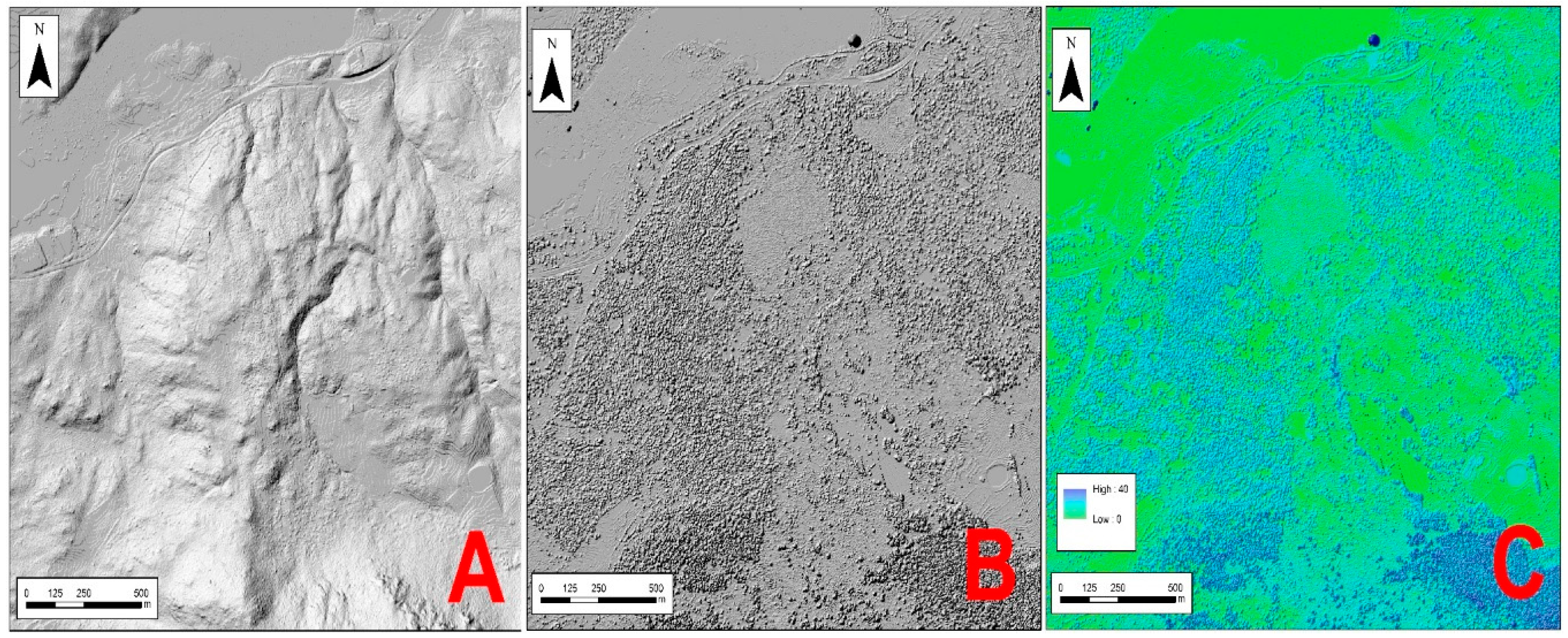
Firstly, the height of the vegetation was calculated [51]; a digital elevation model (DEM) (Figure 5A), by means of the returns from the soil class, and the digital surface model (DMS) (Figure 5B), using only the first returns, are used to accomplish this. Both models are filled in to avoid the possibility of pixels with no data. By subtracting using the Raster Calculator tool in the ArcMap 10.5 Software [52], the height of the vegetation is obtained (Figure 5C).
Then, the three types of FCC are calculated [53]. This is done by creating a LAS dataset of all returns of the soil class, and for each of the three canopy covers depending on the types of return needed (Table 4). The surface occupied by soil and vegetation is added to obtain of total surface, in this step the FCC are calculated (Figure 6).
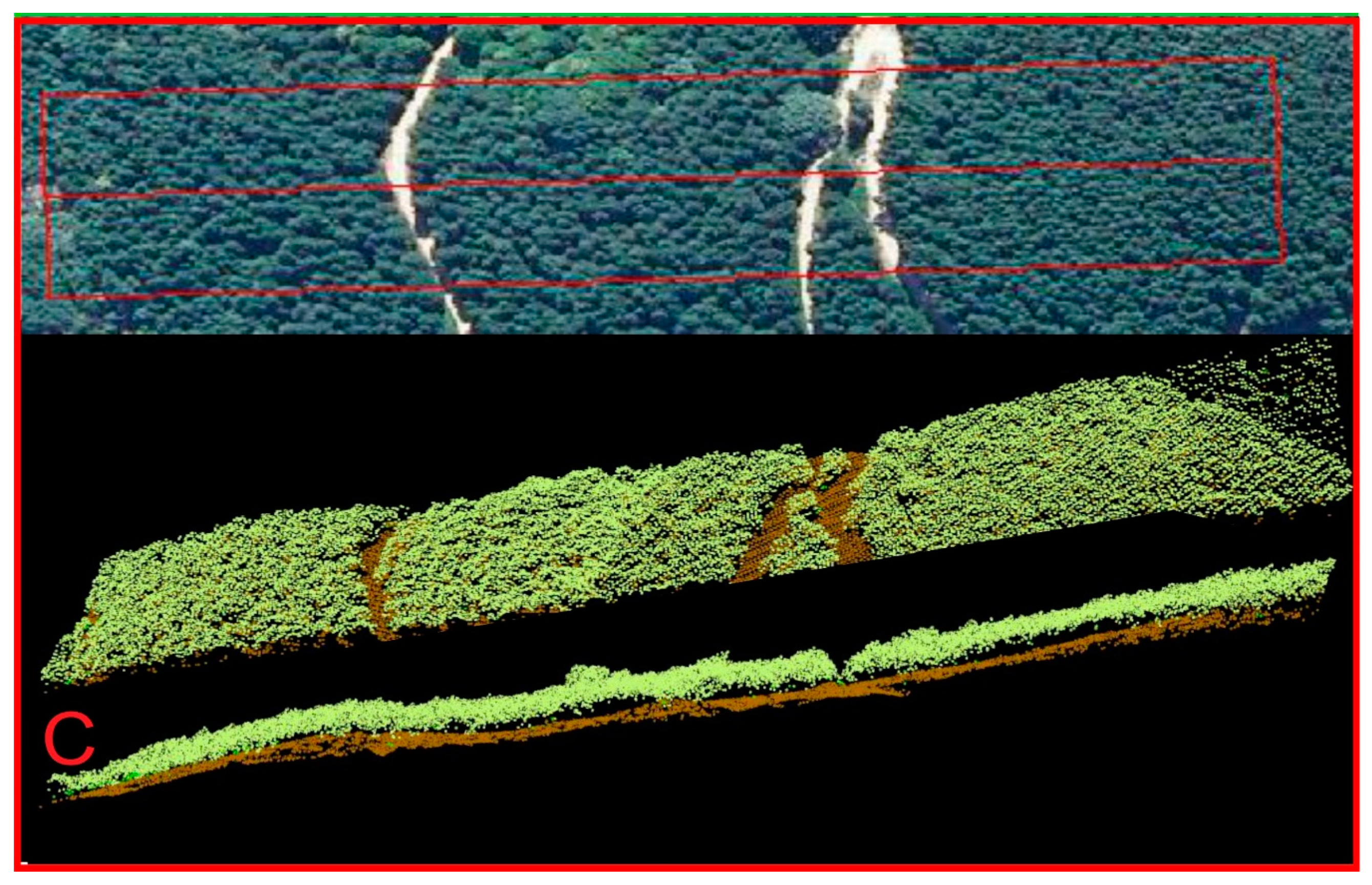
In the LiDAR sections (Figure 7) we can see the different information provided by these data, such as fuel models 0 (for example, urban areas), compared with the increase of the arboreal density of model 1 compared with model 9, as well as its vertical continuity.
Automating the process by the creation of a tool with the Model Builder from ArcGIS software would allow the processing of the LiDAR data in different areas of the study area to be carried out more quickly, and this would facilitate the creation of the mapping since specialist knowledge would not be necessary and processing of LiDAR data with only GIS knowledge would be possible (Figure 8).
2.3.3. Creation of Fuel-Models Mapping
The applied methodology works with the decision algorithms, using the information provided by the different rasters from the LiDAR to characterize the arboreal masses. The raster from the classification of images from Sentinel 2 [54], from vegetation mapping, allows automatic allocation of fuel models to be carried out.
First, the vegetation types (grassland, scrubland, and woodland) are differentiated by the vegetation mapping. Once the vegetation has been differentiated using the ArcGIS mathematical algorithms, the data that characterise the different arboreal masses (height of the vegetation and FCC) are extracted, since the fuel models are based on the structure and distribution of the vegetation. In order to correctly assign the types of fuel models, the following decision tree was designed (Table 5).
2.3.4. Probability Ignition Mapping
The probability of ignition is the chance that a firebrand will cause an ignition when it lands on receptive fuels. It is a hazard index designed by the Instituto para la Conservación de la Naturaleza (ICONA), [55] used since 1987. This index does not take into account the state of the living vegetation, but rather estimates the moisture content of the light and dead fuels located on the forest surface from the air temperature, relative humidity, exposure, and topography.
Creating Trend Maps from Weather Data
From the monthly data from June to September of 2016, obtained from the meteorological stations (Table 6) located in the vicinity of the study area, the maps of average temperatures and average relative humidity were created. For this purpose, the geostatistical tool Inverse Distance Weighting (IDW) is used to generate the corresponding cartography.
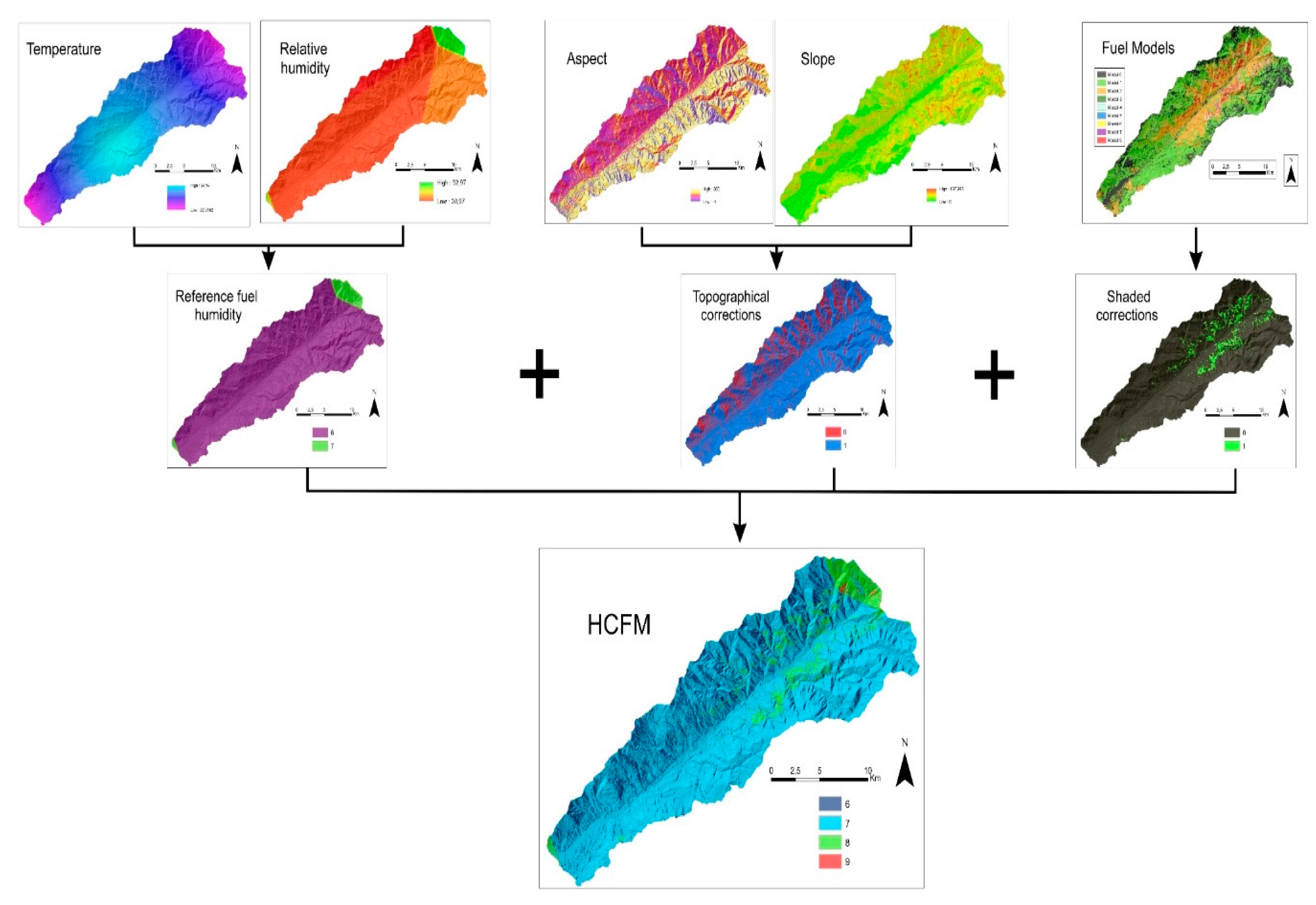
To calculate the humidity of the dead fine fuel (HCFM) (Figure 9), from the relative humidity and temperature, the reference fuel moisture tables are used. The humidity of the dead fine fuel has to be corrected according to the topography characteristics of slope and exposure. To achieve this, the slope and orientations maps are calculated with (digital terrain model) DTM and the pertinent corrections are made with the fine dead fuel moisture tables. Fuel models 8 and 9 are assigned a value of 1 to correct for the humidity of the dead fine fuel due to shading provided by a tree. The rest are assigned a value of 0. Finally, the probability of ignition, which is the probability that a fly ash or ember falling on a dead fine fuel could ignite, is calculated using the reference fuel moisture tables and fuel model mapping [56]. Equation (1) is used for this calculation:
Reference fuel humidity + slope/orientation corrections + shading corrections = HCFM
2.3.5. Validation
The vegetation mapping was validated in the field, with the objectives of calculating the reliability of the same after performing the supervised classification, checking that the data obtained from the LiDAR were correct, and correcting possible anomalies.
The vegetation was verified using 50 points distributed throughout the study area in a random manner, with a minimum extension of 12 adjacent pixels belonging to the same vegetation class; 70% of these areas were used as training areas for the development of the cartography, while the remaining 30% were later used as a test to verify the accuracy of said cartography. To calculate the accuracy of the vegetation mapping, a confusion matrix was made. This is a square matrix that includes as many rows as the types of vegetation we have assigned, and as many columns as the types of vegetation to be analysed in the field. From the percentage of points corresponding to the types of vegetation assigned in relation to the total number of points, and the probability of success of the vegetation assigned in relation to the total number of points, the probability of success of the vegetation mapping was obtained. The Kappa coefficient that adjusts the effect of chance by class crossing was also calculated.
The probability ignition mapping was validated by comparing it with the historical database of wildfire corresponding to the period of climatic data used in the model.
3. Results
3.1. Vegetation Mapping
After performing the supervised classification (Figure 10) vegetation and land-use mapping with a high resolution (pixel of 10 × 10 m) was obtained, with which the fuel models were subsequently calculated.
Table 7 shows the error matrix of vegetation mapping after supervised classification from the nearest neighbor. The overall accuracy was 88% (Kappa index 0.86), which is considered satisfactory in terms of accuracy since it has a large number of classes with some notable similarities between them.
In general, the user’s accuracy and the producer’s accuracy in the individual classes were good since they are very close the unit except specific cases. For example, the village class have a great deal of confusion with rocky class, and the rocky class have a great deal confusion with the oak trees, because it has a large amount of bare soil, of very light colours. However, there are classes with a very high producer’s accuracy such as water, holm oaks, pines forest, chestnut forest, scubland and grassland.
3.2. Creation of Fuel-Models Mapping
Figure 11 shows the mapping generated for the classification of fuel models. The abundant fuel model in the Jerte valley is grassland (model 1 and 2) at 73%. Model 1 is located in areas of greater altitude, in the head and inferior third of the valley, while model 2 is distributed in areas of medium and low height of the upper zones and also in the vicinity of the Plasencia reservoir.
The presence of the other fuel models—scrubland (models 4–7) and little fall (model 9)—is much smaller. Among the scrubland models, it is possible to differentiate between models with a moderate load (models 5 and 6) on the southern slope, although with a very small presence, and the model with a high load (model 7), with small spots scattered in the upper half of the valley. Model 9 is located at a medium height on both slopes due to the presence of chestnut forest (Castanea sativa) and oak forest (Quercus pyrenaica).
It should be kept in mind that model 10 and the models of the remains of cut and other forestry operations (models 11–13) have not been included, since we cannot discriminate whether the remains in the undergrowth are of natural origin (pests or diseases) or due to forest holdings (forestry treatments). The assignment of the type of models associated with wooded masses would only be valid through their field verification, given the temporary nature of these disturbances.
3.3. Ignition-Probability Mapping
The results for ignition-probability mapping (Figure 12) show three differentiated zones with values between 40% and 60%.
The areas with the highest probability of ignition correspond to a lower relative humidity, with values around 40% and within the sun’s slopes. On the other hand, the lower ignition probabilities correspond to the presence of fuel model 9; that is, with oak forest and chestnut forest that provide shade to the underlying materials.
To validate the probability of ignition mapping, it was compared with the inventory of historical fire data in the study area. It was verified that there is indeed a relationship between the increase in the probability of ignition and the volume of outbreak fire. Thus, in the area with a 60% probability of fire, there were 2.79 fires per km2; in the area corresponding to a 50% probability of fire there were 2.23 fires per km2, and in areas of a probability of 40% there were 1.94 fires per km2.
The ignition-probability mapping is the base layer upon which the meteorological risk map of wildfire is built daily in the Regional Operational Centre. It is obtained by combining the probability of ignition with the wind speed, with a correction due to precipitation. The danger calculation procedure is automated on the GIS platforms, so from the presented layer of probability of ignition it is only necessary to update the daily meteorological forecasts to obtain the danger indexes.
4. Discussion
The results of the study support the importance of using remote sensing in wildfire prevention, since the proposed methodology allows us to obtain fuel-model mapping in a short time and with very high accuracy, as well as eliciting the probability of ignition of the different areas with accuracy and daily temporality.
Previous studies have shown that the use of images from Sentinel 2 has been very effective for the classification of both crops and forest vegetation [57]. It is considered a very promising tool for precision agriculture [58] because of its high spatial and temporal resolution, among other features. These images have been used for vegetation classification, obtaining an accuracy of 77% [59]. In the present study, satellite images have been merged with LiDAR data, increasing the accuracy to 88%. Therefore, the use of both technologies in combination is optimal for forestry studies, especially in the field of wildfire. Different studies have reached similar conclusions [60], because the LiDAR information gathers vegetation height data with great accuracy [61], while the satellite images provide information on the texture, radiation, and information of the terrain; this range of information is very useful for mapping. It has also been shown that forestry inventories are much more precise if they have been carried out by unmanned vessels rather than by field work [62], which makes this methodology faster, more economical, and more reliable.
Once vegetation mapping of a high accuracy has been obtained, and the fuel-model mapping is generated, it becomes possible to enter the data into different programs for the calculation of the behaviour of fires while also taking into account the climatic and topographic data [63].
5. Conclusions
The methodology described in this paper allows us to obtain fuel-model mapping with a high level of detail from structural information of the vegetation, provided by LiDAR data in combination with Sentinel 2 images. This method allows the generation of fuel-model mapping of large extensions at a very low cost, given that field work is reduced to a minimum, which allows permanent ongoing updating to occur.
Furthermore, this methodology allows us to obtain high-resolution and detailed inputs (cells of 10 × 10 m), greater than those of any mapping used prior to this, for the purpose of developing forest fire simulation software that makes it possible to anticipate with greater certainty the behaviour of potential fires.
From this work, it is concluded that the probability determined from ignition mapping allows us to generate daily maps of the danger index based on up to date meteorological forecasts with GIS scripts. This automates the process and improves the historical cartographies of fuel models and the danger of ignition, which in turn makes it possible to assess the redistribution of operational difficulties according to the mapping outputs, especially in times of low and medium danger where the devices are not fully operational.
This mapping is a preventive measure to avoid wildfires and serves as an essential tool in the planning and management of the territory, and as a decision-making tool when planning preventive forestry treatments, construction of infrastructure, etc.
Acknowledgments
This work has been supported by the USAL research projects CGL2012-37281-C02.01, CGL2015-67169-P and CGL2015-69919-R (MINECO-FEDER).
Author Contributions
All authors were responsible for the design of the research. Y.S.S., A.M.-G. and F.S.F. developed the GIS data and analyzed the digitals maps: Lidar treatment and remote sensing; and M.M.P. the index of vegetation and fuel model. All authors contributed to writing the paper and to the discussion of the analysis.
Conflicts of Interest
The authors declare no conflicts of interest.
References
- González-Delgado, J.A.; Martínez-Graña, A.M.; Civis, J.; Sierro, F.J.; Goy, J.L.; Dabrio, C.F.; Ruiz, F.; González-Regalado, M.L.; Abad, M. Virtual 3D tour of the Neogene palaeontological heritage of Huelva (Guadalquivir Basin, Spain). Environ. Earth Sci. 2015, 73, 4609–4618. [Google Scholar] [CrossRef]
- San-Miguel Ayanz, J.; Moreno, J.; Camia, A. Analysis of large fires in European Mediterranean landscapes: Lessons learned and perpective. Forest Ecol. Manag. 2013, 11–22. [Google Scholar] [CrossRef]
- Martínez-Graña, A.M.; González-Delgado, J.A.; Pallarés, S.; Goy, J.L.; Civis, J. 3D Virtual Itinerary for Education Using Google Earth as a Tool for the Recovery of the Geological Heritage of Natural Areas: Application in the “Las Batuecas Valley” Nature Park (Salamanca, Spain). Sustainability 2014, 6, 8567–8591. [Google Scholar] [CrossRef]
- Koutsias, N.; Karteris, M. Classification analyses of vegetation for delineating forest fire fuel complexes in a Mediterranean test site using satellite remote sensing and GIS. Int. J. Remote Sens. 2003, 24, 3093–3104. [Google Scholar] [CrossRef]
- Bastarrika, A.; Alvarado, M.; Artano, K.; Martinez, M.; Mesanza, A.; Torre, L.; Ramo, R.; Chuvieco, E. BAMS: A Tool for Supervised Burned Area Mapping Using Landsat Data. Remote Sens. 2014, 6, 12360–12380. [Google Scholar] [CrossRef]
- Chuvieco, E.; Yue, C.; Heil, A.; Mouillot, F.; Alonso-Canas, I.; Padilla, M.; Tansey, K. A new global burned area product for climate assessment of fire impacts. Glob. Ecol. Biogeogr. 2016, 1–11. [Google Scholar] [CrossRef]
- Sánchez, Y.; Martínez-Graña, A.; Santos Francés, F.; Yenes, M. Influence of the sediment delivery ratio indexo n the Analysis of silting and break risk in the Plasencia reservoir (Central System, Spain). Nat. Hazards 2018. [Google Scholar] [CrossRef]
- Fernandez-Manso, A.; Fernandez-Manso, O.; Quintano, C. SENTINEL-2A red-edge spectral indices suitability for discriminating burn severity. Int. J. Appl. Earth Obs. Geoinf. 2016, 50, 170–175. [Google Scholar] [CrossRef]
- Nogueira, J.M.P.; Ruffault, J.; Chuvieco, E.; Mouillot, F. Can we go beyong burned area in th assessment of global remote sensing products with fire patch metrics? Remote Sens. 2016, 9, 7. [Google Scholar] [CrossRef]
- Verhegghen, A.; Eva, H.; Ceccherini, G.; Achard, F.; Gond, V.; Gourlet-Fleury, S.; Omar Cerutti, P. The Potential os Sentinel Satellites for Burnt Area Mapping and Monitoring in the Congo Basin Forests. Remote Sens. 2016, 8, 986. [Google Scholar]
- Lumbierres, M.; Méndez, P.F.; Bustamante, J.; Sorieguer, R.; Santamaría, L. Modeling Biomass Production in seasonal wetlands using MODIS NDVI Land Surface Phonology. Remote Sens. 2017, 9, 392. [Google Scholar] [CrossRef]
- Navarro, G.; Caballero, I.; Silva, G.; Parra, P.; Vazquez, A.; Caldeira, R. Evaluation of forest fire on Madeira Island using Sentinel-2A MSI imagery. Int. J. Appl. Earth Obs. Geoinf. 2017, 58, 97–106. [Google Scholar] [CrossRef]
- Schoroeder, W.; Oliva, P.; Giglio, L.; Quayle, B.; Lorenz, E.; Morelli, F. Active fire detecction using Landsat-8/OLI data. Remote Sens. Environ. 2016, 185, 210–220. [Google Scholar] [CrossRef]
- Riaño, D.; Chuvieco, E.; Salas, J.; Palacios-Orueta, A.; Bastarrica, A. Generation of fuel types maps from Landsat TM Images and ancillary data in mediterranean ecosystem. Can. J. Forest Res. 2002, 32, 1301–1315. [Google Scholar] [CrossRef]
- Mata, T.; Burriel, J.; Ibáñez, J.; Vayreda, J. Mapas de Modelos de Combustibles y Modelos de Inflamabilidad en Cataluña; Wildfire: Sevilla, Spain, 2007. [Google Scholar]
- Andersen, H.E.; McGaughey, R.J.; Reutebuch, S.E. Estimating forest canopy fuel parameters using LiDAR data. Remote Sens. Environ. 2005, 94, 441–449. [Google Scholar] [CrossRef]
- Ferraz, A.B. 3-D Mapping of a multi-layered Mediterranean forest using ALS data. Remote Sens. Environ. 2012, 121, 210–223. [Google Scholar] [CrossRef]
- Gonzalez-Olabarria, J.; Rodriguez, F.; Fernadez-Landa, A.; Mola-Yudego, B. Mapping fires risk in the Model Forest of Urbión (Spain) based on airbone LiDAR measurements. Forest Ecol. Manag. 2012, 282, 149–156. [Google Scholar] [CrossRef]
- Erdody, T.L.; Moskal, M. Fusion of LiDAR and imagery for estimating forest canopy fuels. Remote Sens. Environ. 2010, 114, 725–737. [Google Scholar] [CrossRef]
- Kramer, H.C. Quantifying Ladder Fuels: A New Approach Using LiDAR. Forest 2014, 5, 1432–1453. [Google Scholar] [CrossRef]
- Kane, V.; Cansler, C.; Povak, N.; Kane, J.; McGaughey, R.; Lutz, J.; North, M. Mixed severity fire effects within the Rim fire: Relative importance of local climate, fire weather, topography, and forest estructure. Forest Ecol. Manag. 2015, 358, 62–79. [Google Scholar] [CrossRef]
- Contreras, M.A.; Parsons, R.; Chung, W. Modeling tree- level fuel connectiviti to evaluate the effectiveness of thinning treatments for reducing crown fire potencial. Forest Ecol. Manag. 2012, 264, 134–149. [Google Scholar] [CrossRef]
- Martinez-Graña, A.M.; Goy, J.L.; Cimarra, C. 2D to 3D geologic map transformation using virtual globes and flight simulators and their applications in the analysis of geodiversity in natural areas. Environ. Earth Sci. 2015, 73, 8023–8034. [Google Scholar] [CrossRef]
- Carla De Grandi, E.; Mitchard, E.; Hoekman, D. Wavelet Based Analysis of TanDEM-X and LiDAR DEMs across a Tropical Vegetation Heterogeneity Gradient Driven by Fire Disturbance in Indonesia. Remote Sens. 2016, 8, 641. [Google Scholar] [CrossRef]
- Mutlu, M.; Popescu, S.C.; Stripling, C.; Spencer, T. Mapping surface fuel models using LiDAR and multispectral data fusion for fire behavior. Remote Sens. Environ. 2008, 112, 274–285. [Google Scholar] [CrossRef]
- Mutlu, M.; Popescu, S.C.; Zhao, K. Sensitive analysis of fire behaviour modelling with LiDAR- derived surface fuel maps. Forest Ecol. Manag. 2008, 256, 289–294. [Google Scholar] [CrossRef]
- Novozhilov, V. Fire Hazards of some modern Solid Fuels. Energies 2017, 10, 113. [Google Scholar] [CrossRef]
- Simpson, J.E.; Wooster, M.; Smith, T.E.; Triverdi, M.; Vernimmen, R.R.; Dedi, R.; Dinata, Y. Tropical Peatland Burn Depth and Combustion Heterogeneity Assessed Using UAV Photogrammetry and Airbone Lidar. Remote Sens. 2016, 8, 1000. [Google Scholar] [CrossRef]
- Eskandari, S.C. Fire danger assessment in Iran based geospatial information. Int. J. Appl. Earth Obs. Geoinf. 2015, 42, 57–64. [Google Scholar] [CrossRef]
- Martínez-Graña, A.; Boski, T.; Goy, J.L.; Zazo, C.; Dabrio, C.J. Coastal-flood risk management in central Algarve: Vulnerability and flood risk indices (South Portugal). Ecol. Indic. 2016, 71, 302–316. [Google Scholar] [CrossRef]
- Yan, L.; Roy, D.P.; Zhang, H.; Li, J.; Huang, H. An automated aproach for sub-pixel registration of landsat-8 Operational Land Imager (OLI) and Sentinel-2 Multi Spectral Instrument (MSI) Imagery. Remote Sens. 2016, 8, 520. [Google Scholar] [CrossRef]
- Vaglio Laurin, G.; Pirotti, F.; Callegari, M.; Chen, M.; Cuozzon, G.; Lingua, E.; Papale, D. Potential ALOS2 and NDVI to Estimate Forest Above- Ground Biomass, and Comparison with LiDAR-Derived Estimates. Remote Sens. 2016, 9, 18. [Google Scholar] [CrossRef]
- Martínez-Graña, A.M.; Goy, J.L.; De Bustamante, I.; Zazo, C. Characterisation of environmental impact on resources, using strategic assessment of environmental impact and management of natural spaces of “Las Batuecas-Sierra de Francia” and “Quilamas” (Salamanca, Spain). Environ. Earth Sci. 2014, 71, 39–51. [Google Scholar]
- Aguado, I.; Camia, A. Fundamentos y utilización de índices meteorológicos de peligro de incendio. Serie Geogr. 1998, 7, 49–58. [Google Scholar]
- Carrasco González, R. Geomorfología del Valle del Jerte. Las líneas Maestras del Paisaje. Diss. Ph.D. Thesis, Universidad de Extremadura, Cáceres, Spain, 2000. [Google Scholar]
- SiAR, S.D. Ministerio de Agricultura y Pesca, Alimentación y Medio Ambiente. Available online: http://eportal.mapama.gob.es/websiar/Inicio.aspx (accessed on 2 May 2017).
- Mandanici, E.; Biteli, G. Preliminary Comparison of Sentinel-2 and Landsat 8. Remote Sens. 2016, 8, 1014. [Google Scholar] [CrossRef]
- Norman, S.P.; Hargrove, W.W.; Christie, W.M. Spring and Autumn Phenological VAriability across Enviromental Gradients of Great Smoky Mountains National, Park, USA. Remote Sens. 2017, 9, 407. [Google Scholar] [CrossRef]
- ESA. Copernicus. (European Space Agency) Obtenido de Observing the Earth. Available online: http://www.esa.int/Our_Activities/Observing_the_Earth/Copernicus/Sentinel-2 (accessed on 3 May 2017).
- Blanco, J.; Gracía, D.; Castellnou, M.; Grillo, F. Curso Básico de Incendios Forestales; Universidad de Lérida: Lérida, Spain, 2007. [Google Scholar]
- Albini, F.A. Estimating Wildfire Behaviour and Effects; General Technical Report; Departament of Agriculture, Forest Service, Intermountain Forest and a Range Experiment Station: Ogden, UT, USA, 1976; 92p.
- Burgan, R.; Rothermel, R. BEHAVE: Fire Behaviur Prediction and Fuel Modelling System-Fuel Subsystem; USDA Forest Service: Ogden, UT, USA, 1984.
- Rothermel, R. How to Predict the Spread and Intensity of Forest and Range Fires; US Department of Agriculture, Forest Service, Intermountain Forest and Range Experiment Station: Ogden, UT, USA, 1983.
- Anderson, H.E. Aids to Determining Fuel Models for Estimating Fire Behaviour; General Technical Report; US Department of Agriculture-Forest Service, Intermountain Research Station: Ogden, UT, USA, 1982; pp. 1–22.
- Gascon, F.; Bouzinac, C.; Thepaut, O.; Jung, M.; Francesconi, B.; Louis, J.; Cadau, E. Copernicus Sentinel 2A Calibration a Products VAlidation Status. Remote Sens. 2017, 9, 584. [Google Scholar] [CrossRef]
- Hollstein, A.S. Ready-to-Use Methods for the Detection of Clouds, Cirrus, Snow, Shadow, Water and Clear Sky Pixels in Sentinel-2 MSI Images. Remote Sens. 2016, 8, 666. [Google Scholar] [CrossRef]
- Team, Q.D. Quantum GIS Geosgraphic Information System. Open Source Geospatial Fundation Project. Obtenido de. Available online: http://qgis.osgeo.org (accessed on 15 December 2016).
- Congedo, L. Semi-Automatic Classification Plugin Documentation. Release 5.3.6.1. 2018. Available online: https://media.readthedocs.org/pdf/semiautomaticclassificationmanual-v5/latest/semiautomaticclassificationmanual-v5.pdf (accessed on 9 March 2018).
- Spits, C.; Wallace, L.; Reinke, K. Investigating Surface and Near-Surface Bushfire Fuel Attributes: A Comparison between Visual Assessments and Image-Based Point Clouds. Sensors 2017, 17, 910. [Google Scholar] [CrossRef] [PubMed]
- Amani, M.; Salehi, B.; Mahdavi, S.; Granger, J. Spectral Analysis of wetlands in Newfoundland using Sentinel 2A and Landsat 8 imagery. In Proceedings of the IGTF 2017-Imaging & Geospatial Technology Forum: ASPRS Annual Conference, Baltimore, MD, USA, 12–16 March 2017. [Google Scholar]
- García, M.; Riaño, D.; Chuvieco, E.; Salas, J.; Mark Danson, F. Multiespectral and LiDAR data fusion for furl type mapping using Support Vector Machine and decision rules. Remote Sens. Environ. 2011, 115, 1369–1379. [Google Scholar] [CrossRef]
- ESRI. ArcGIS Desktop 10.5; Environmental Systems Research Institute: Redlands, CA, USA, 2017. [Google Scholar]
- Marino, E.; Ranz, P.; Tomé, J.; Noriega, M.; Esteban, J.; Madrigal, J. Generation of high-resolution fuel model maps from discrete airborne laser scanner and Landsat-8 OLI: A low-cost and highly updated methodology for large areas. Remote Sens. Environ. 2016, 267–280. [Google Scholar] [CrossRef]
- Molina, D.M.; Bardají, M.; Castellnou, M. Probabilidad de Ignición, grandes incendios y dificultad de extinción. Ecología 1998, 12, 333–350. [Google Scholar]
- Alonso-Benito, A.; Arroyo, L.; Arbelo, M.; Hernandez-Leal, P. Fusion of world View-2 and LiDAR Data to Map Fuel Types in the Canary Islands. Remote Sens. 2016, 8, 669. [Google Scholar] [CrossRef]
- Pettinari, M.; Chuvieco, E. Cartografía de combustible y potenciales de incendios en el continente africano utilizando FCCS. Rev. Teledetec. 2015, 43, 1–10. [Google Scholar] [CrossRef]
- Immitzer, M.V. First Experience with Sentinel-2 Data for Crop and Tree Species Classifications in Central Europe. Remote Sens. 2016, 8, 166. [Google Scholar] [CrossRef]
- Escolà, A.; Badia, N.; Arnó, J.; Martínez-Casasnovas, J. Using Sentinel-2 imagen to implement Precision Agriculture techniques in large arable fields. First result of a case study. Adv. Anim. Biosci. 2017, 377–382. [Google Scholar] [CrossRef]
- Kupková, L.; Cervena, L.; Suchá, R.; Jakesová, L.; Zagajewski, B.; Brezina, S.; Albrechtová, J. Classification of tundra vegetation in the Krkonose Mts. National Park Using APEX, AISA Dual and Sentinel 2-a Data. Eur. J. Remote Sens. 2017, 50, 30–46. [Google Scholar] [CrossRef]
- Liu, K.; Wang, J.; Zeng, W.; Song, J. Comparison and Evaluation of Three Methods for Estimating Forest above Ground Biomass Using TM and GLAS Data. Remote Sens. 2017, 9, 341. [Google Scholar] [CrossRef]
- Gopalakrishnan, R.; Thomas, V.A.; Coulston, J.W.; Wynne, R.H. Prediction of Canopy Heights over a Large Region Using Heterogeneous Lidar Dataset: Efficacy and Challenges. Remote Sens. 2015, 7, 11036–11060. [Google Scholar] [CrossRef]
- Jones Kachamba, D.; Ole Orka, H.; Naesset, E.; Eid, T.; Gobakken, T. Influence of Plot Size on Efficiency of Biomass Estimates in Inventtories of Dry Tropical Forest Assisted by Photogrammetric Data from an Unmanned Aircraft System. Remote Sens. 2017, 9, 610. [Google Scholar] [CrossRef]
- Lucrecia Pettinari, M.; Chuvieco, E. Fire Behavior Simulation from Global Fuel and Climatic Information. Forest 2017, 8, 179. [Google Scholar] [CrossRef]
Figure 1.
Location of the study area (the Jerte valley) within Cáceres (Spain).

Figure 2.
Methodological diagram.

Figure 3.
Situation of training areas.

Figure 4.
Spectral signature of the different types of vegetation and land uses in relation to wavelength (μm) by Sentinel 2 satellite bands.
Figure 4.
Spectral signature of the different types of vegetation and land uses in relation to wavelength (μm) by Sentinel 2 satellite bands.

Figure 5.
(A) Digital terrain model (DTM); (B) digital surface model (DSM); (C) height of the vegetation.
Figure 5.
(A) Digital terrain model (DTM); (B) digital surface model (DSM); (C) height of the vegetation.

Figure 6.
Types of canopy cover.

Figure 7.
LiDAR section each section is composed by the orthophoto, The section LiDAR in oblique view and the LiDAR section in vertical view. (A) Model 0: Towns and infrastructure; (B) Model 1: FCC < 0.3; (C) Model 9: FCCc > 0.3 FCCs < 0.3.
Figure 7.
LiDAR section each section is composed by the orthophoto, The section LiDAR in oblique view and the LiDAR section in vertical view. (A) Model 0: Towns and infrastructure; (B) Model 1: FCC < 0.3; (C) Model 9: FCCc > 0.3 FCCs < 0.3.


Figure 8.
General calculation process of the FCC in Model Builder.

Figure 9.
Humidity of the dead fine fuel (HCFM) calculation process.

Figure 10.
Land-use and vegetation mapping.

Figure 11.
Fuel-models mapping.

Figure 12.
Probability of ignition mapping.


Table 1.
Radiometric and spatial resolution of Sentinel 2.
| SENTINEL-2 Radiometric and Spatial Resolutions | |||
|---|---|---|---|
| Band Number | Name | Central Wavelength (nm) | Spatial Resolution (m) |
| 1 | aerosols | 443 | 60 |
| 2 | blue | 490 | 10 |
| 3 | green | 560 | 10 |
| 4 | red | 665 | 10 |
| 5 | NIR | 705 | 20 |
| 6 | NIR | 740 | 20 |
| 7 | NIR | 783 | 20 |
| 8 | NIR | 842 | 10 |
| 8a | NIR | 865 | 20 |
| 9 | Water vapour | 945 | 60 |
| 10 | Cirrus detection | 1375 | 60 |
| 11 | SWIR | 1610 | 20 |
| 12 | SWIR | 2190 | 20 |
Table 2.
LiDAR sensor specifications.
| Camera | Aerial Orthophotography |
|---|---|
| Laser spectral band | panchromatic, blue, green and red |
| Laser pulse density | 2 points/m2 |
| The pixel size | 0.20 m |
| Flying height | Maximum 3000m |
| Horizontal accuracy | 0.30 m |
| Vertical accuracy | 0.20m |
Table 3.
Characteristics of fuel models.
| Type | Model | Short Description |
|---|---|---|
| Urban area | 0 | Infrastructures and towns |
| Grasslands | 1 | Fine dry grass, with possible appearance of herbaceous plants covering a smaller area up to 1/3. Fuel load from 1 to 2 T/ha |
| 2 | Fine dry grass, with clear presence of bushes and trees that cover an area of 1/3 to 2/3. Fuel load of 5 to 10 T/ha | |
| 3 | Coarse, dense, dry and high grass (>1 m). Fuel load of 4 to 6 T/ha. | |
| Scrubland | 4 | Very dense or young thicket repopulate without performances. Fuel load of 25 to 35 T/ha |
| 5 | Dense and green undergrowth less than 0.6 m high. Fuel load of 5 to 8 T/ha. | |
| 6 | Scrub older than model 5 with heights between 0.6 y 1.2 m. Fuel load of 10 to 15 T/ha. | |
| 7 | Flammable species (heath, jars) as the understory of conifers or hardwoods. Fuel load of 10 to 15 T/ha. | |
| Lush leaf under trees | 8 | Dense forest of conifers and hardwoods with compact leaf litter. Fuel load of 10 to 12 T/ha. |
| 9 | Forests with less compact leaf litter, long-leaf conifers, and broadleaved conifers. Fuel load of 7 to 9 T/ha. | |
| 10 | Dense forest with dead wood or infected forest. Fuel load of 30 to 35 T/ha. | |
| Remains of cut and other forestry operations | 11 | Clear and strongly clear forest. Fuel load of 25 to 30 T/ha. |
| 12 | Predominance of remains on the trees. Fuel load of 50 to 80 T/ha. | |
| 13 | Accumulations of thick and heavy debris covering the ground. Fuel load of 100 to 150 T/ha. |
Table 4.
Calculations of canopy cover fraction (FCC) types.
| FCCg | Canopy cover fraction | |
| FCCc | Canopy cover fraction overstory | |
| FCCs | Canopy cover fraction understory |
Table 5.
Decision tree for the classification of fuel models.
| FCC < 1/3 | M1 | ||
| FCC 1/3–2/3 | M2 | ||
| FCC > 2/3 | grassland | M3 | |
| scrubland | >2 m | M4 | |
| <0.6 m | M5 | ||
| >0.6 (0.6–1.2) | M6 | ||
| FCC overstory > 0.3 FCC understory > 0.3 0.6–2 m understory or inflammable scrubland | M7 | ||
| woodland without understory | P. sylvestris | M8 | |
| FCC overstory > 0.3 FCC understory < 0.3 Castanea sativa, Quercus sp; P. pinaster | M9 | ||
Table 6.
Stations data.
| Stations | Average Temperature (°C) | Average Humidity (%) | Coordinate X (m) | Coordinate Y (m) |
|---|---|---|---|---|
| Losar del Barco | 20.1 | 52.9 | 285,381 | 4,472,220 |
| Valdeastillas | 24.5 | 39.8 | 255,607 | 4,447,376 |
| Gargantilla | 24.0 | 38.9 | 249,777 | 4,458,446 |
| Jarandilla de la Vera | 24.0 | 41.8 | 274,426 | 4,442,377 |
| Aldehuela del Jerte | 19.1 | 48.1 | 736,412 | 4,433,680 |
Table 7.
Error matrix of vegetation mapping.
| Reference Data | Total | User’s Accuracy (%) | Kappa | ||||||||||||
|---|---|---|---|---|---|---|---|---|---|---|---|---|---|---|---|
| Water | Castanea sativa | Prunus avium | Quercus ilex | Shrublands | Grasslands | Pinus pinaster | Village | Quercus pyrenaica | Rocky | Bare Soil | |||||
| Classified Data | Water | 6 | 0 | 0 | 0 | 0 | 1 | 0 | 1 | 1 | 0 | 1 | 10 | 0.60 | 0 |
| Castanea sativa | 0 | 22 | 0 | 0 | 0 | 1 | 0 | 0 | 1 | 0 | 0 | 24 | 0.92 | 0 | |
| Prunus avium | 0 | 1 | 102 | 1 | 2 | 2 | 0 | 1 | 1 | 3 | 7 | 120 | 0.85 | 0 | |
| Quercus ilex | 0 | 0 | 2 | 65 | 5 | 2 | 0 | 0 | 2 | 12 | 3 | 91 | 0.71 | 0 | |
| Shrublands | 0 | 0 | 0 | 0 | 59 | 0 | 0 | 0 | 0 | 0 | 0 | 59 | 1.00 | 0 | |
| Grasslands | 0 | 0 | 0 | 0 | 0 | 50 | 0 | 0 | 0 | 0 | 0 | 50 | 1.00 | 0 | |
| Pinus pinaster | 0 | 0 | 0 | 0 | 0 | 0 | 18 | 0 | 0 | 0 | 0 | 18 | 1.00 | 0 | |
| Village | 0 | 0 | 0 | 0 | 0 | 1 | 0 | 5 | 1 | 0 | 3 | 10 | 0.50 | 0 | |
| Quercus pyrenaica | 0 | 0 | 0 | 0 | 0 | 0 | 0 | 0 | 36 | 0 | 0 | 36 | 1.00 | 0 | |
| Rocky | 0 | 0 | 0 | 0 | 0 | 1 | 0 | 3 | 0 | 26 | 0 | 30 | 0.87 | 0 | |
| Bare Soil | 0 | 0 | 0 | 0 | 0 | 0 | 0 | 0 | 0 | 0 | 56 | 56 | 1.00 | 0 | |
| Total | 6 | 23 | 104 | 66 | 66 | 58 | 18 | 10 | 42 | 41 | 70 | 504 | 0.00 | 0 | |
| Producer’s Accuracy | 1.00 | 0.96 | 0.98 | 0.98 | 0.89 | 0.86 | 1.00 | 0.50 | 0.86 | 0.63 | 0.80 | 0 | 0.88 | 0 | |
| Kappa | 0 | 0 | 0 | 0 | 0 | 0 | 0 | 0 | 0 | 0 | 0 | 0 | 0 | 0.86 | |
© 2018 by the authors. Licensee MDPI, Basel, Switzerland. This article is an open access article distributed under the terms and conditions of the Creative Commons Attribution (CC BY) license (http://creativecommons.org/licenses/by/4.0/).
Share and Cite
MDPI and ACS Style
Sánchez Sánchez, Y.; Martínez-Graña, A.; Santos Francés, F.; Mateos Picado, M. Mapping Wildfire Ignition Probability Using Sentinel 2 and LiDAR (Jerte Valley, Cáceres, Spain). Sensors 2018, 18, 826. https://doi.org/10.3390/s18030826
AMA Style
Sánchez Sánchez Y, Martínez-Graña A, Santos Francés F, Mateos Picado M. Mapping Wildfire Ignition Probability Using Sentinel 2 and LiDAR (Jerte Valley, Cáceres, Spain). Sensors. 2018; 18(3):826. https://doi.org/10.3390/s18030826
Chicago/Turabian StyleSánchez Sánchez, Yolanda, Antonio Martínez-Graña, Fernando Santos Francés, and Marina Mateos Picado. 2018. "Mapping Wildfire Ignition Probability Using Sentinel 2 and LiDAR (Jerte Valley, Cáceres, Spain)" Sensors 18, no. 3: 826. https://doi.org/10.3390/s18030826
Note that from the first issue of 2016, this journal uses article numbers instead of page numbers. See further details here.