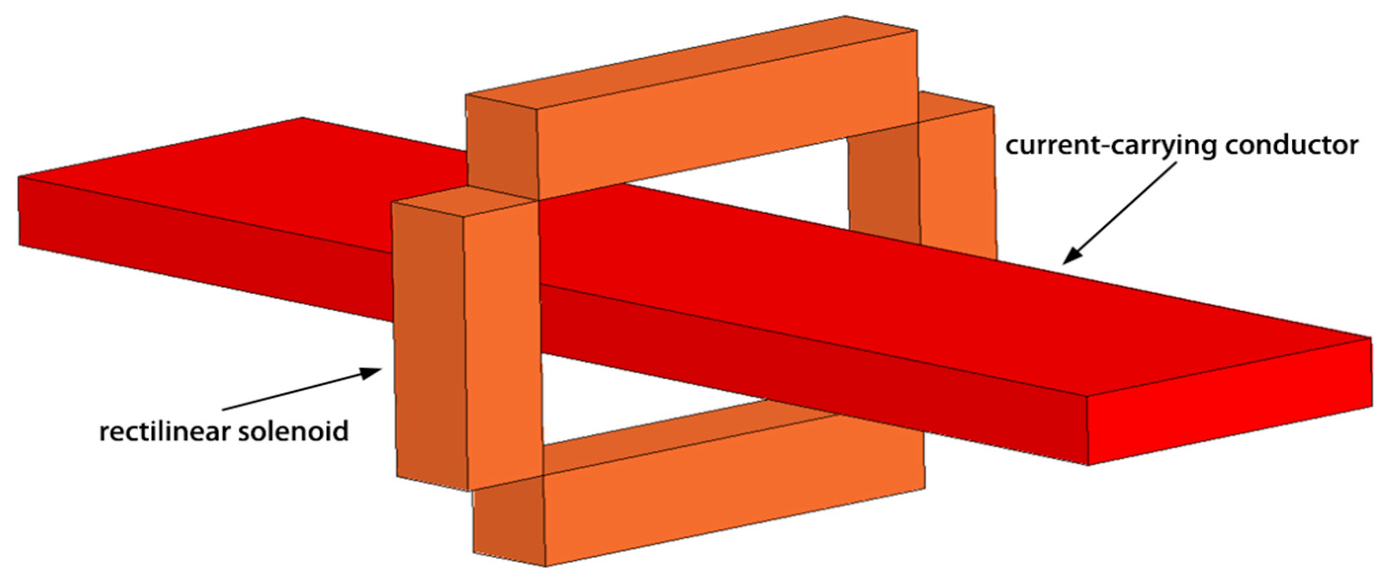
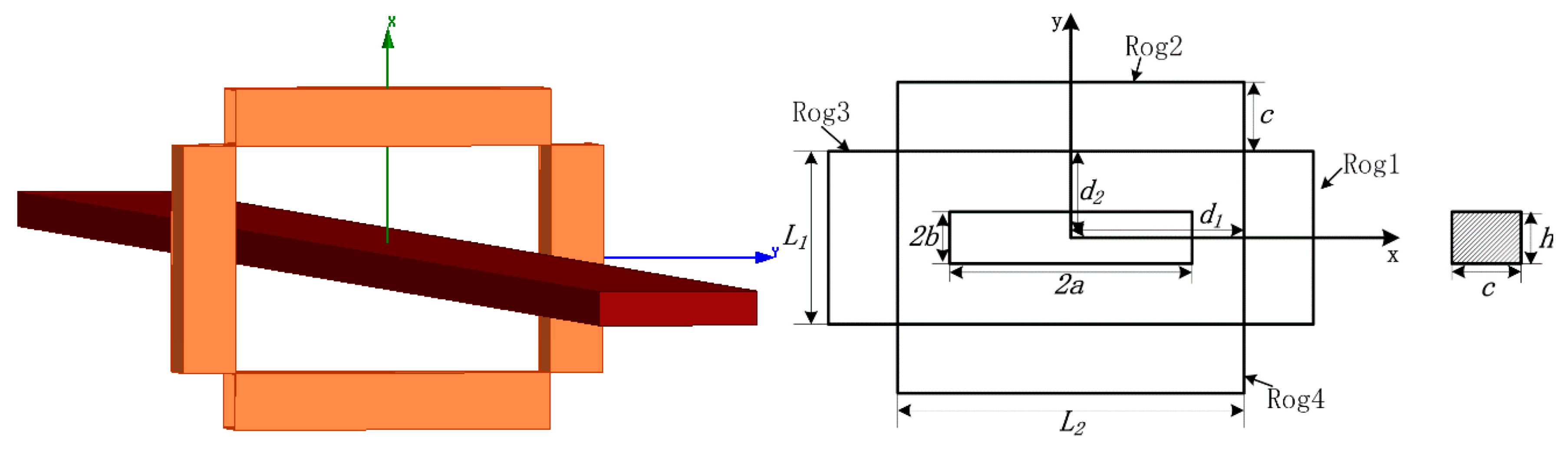
Figure 1.
Model of a discrete RC made of four rectilinear solenoids.
Figure 1.
Model of a discrete RC made of four rectilinear solenoids.
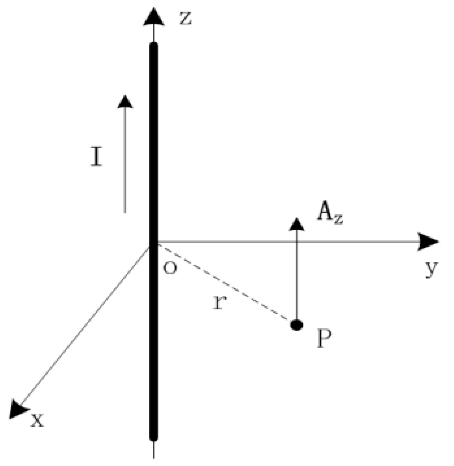
Figure 2.
Magnetic vector potential A at one point in space.
Figure 2.
Magnetic vector potential A at one point in space.
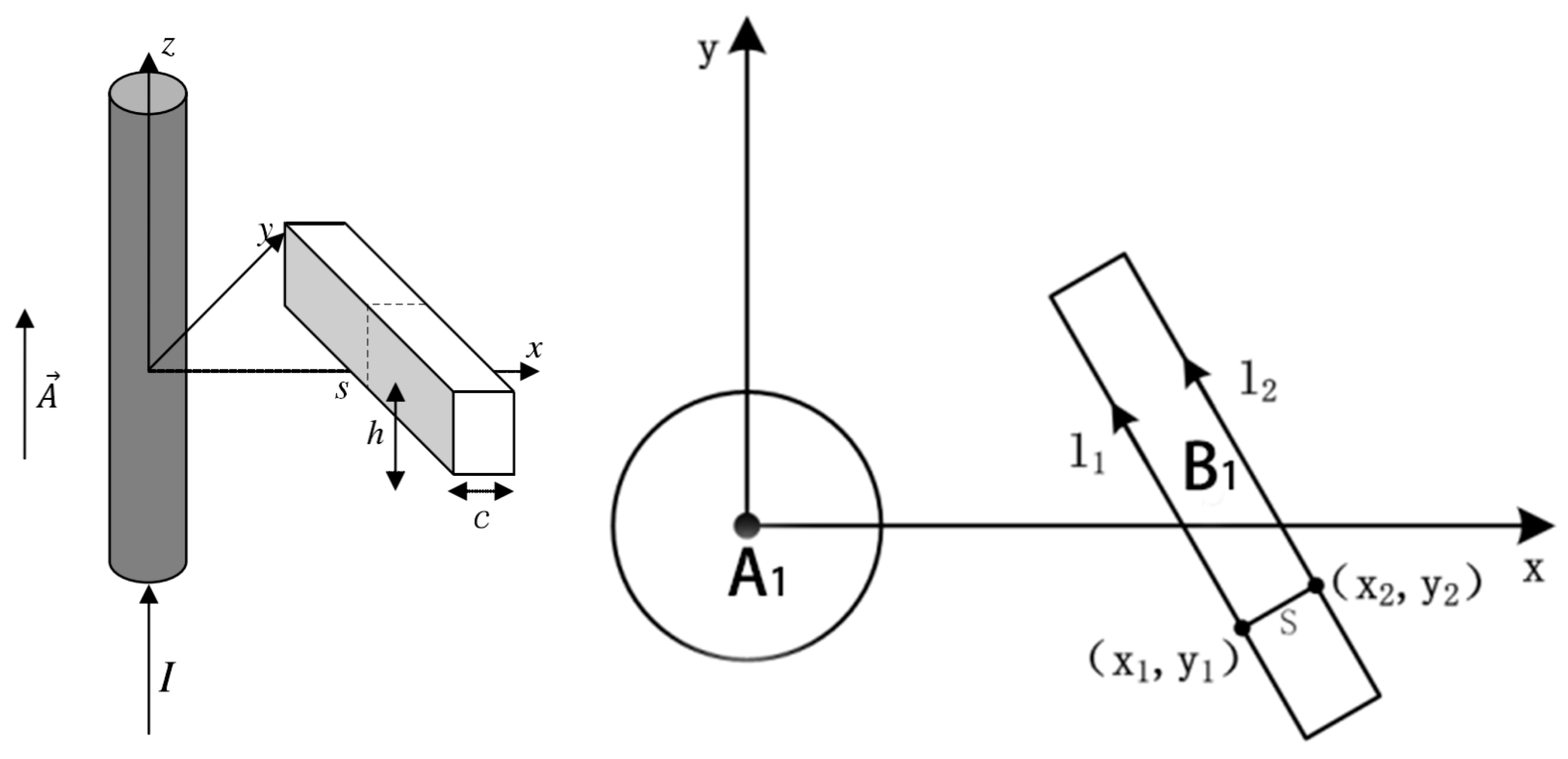
Figure 3.
Model of the conductor and rectilinear solenoid.
Figure 3.
Model of the conductor and rectilinear solenoid.
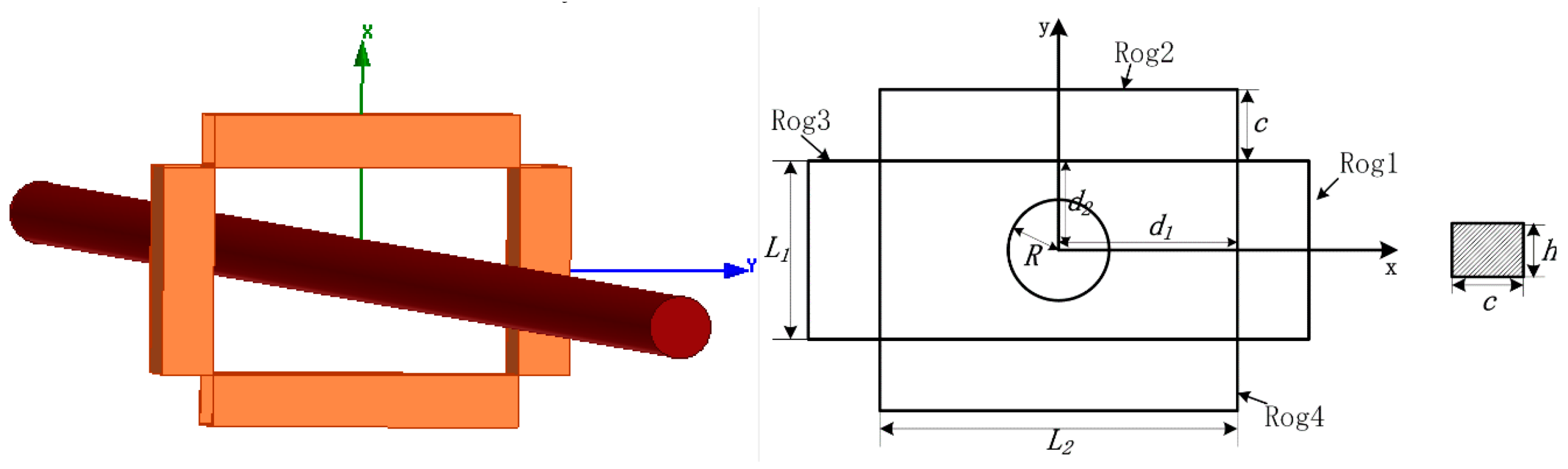
Figure 4.
Model of a circular conductor and a discrete RC, with R = 3 mm, c = 4 mm, h = 3 mm, L1 = 10 mm, L2 = 20 mm, d1 = 10 mm, d2 = 5 mm, ρ (winding density) = 50 turns/mm.
Figure 4.
Model of a circular conductor and a discrete RC, with R = 3 mm, c = 4 mm, h = 3 mm, L1 = 10 mm, L2 = 20 mm, d1 = 10 mm, d2 = 5 mm, ρ (winding density) = 50 turns/mm.
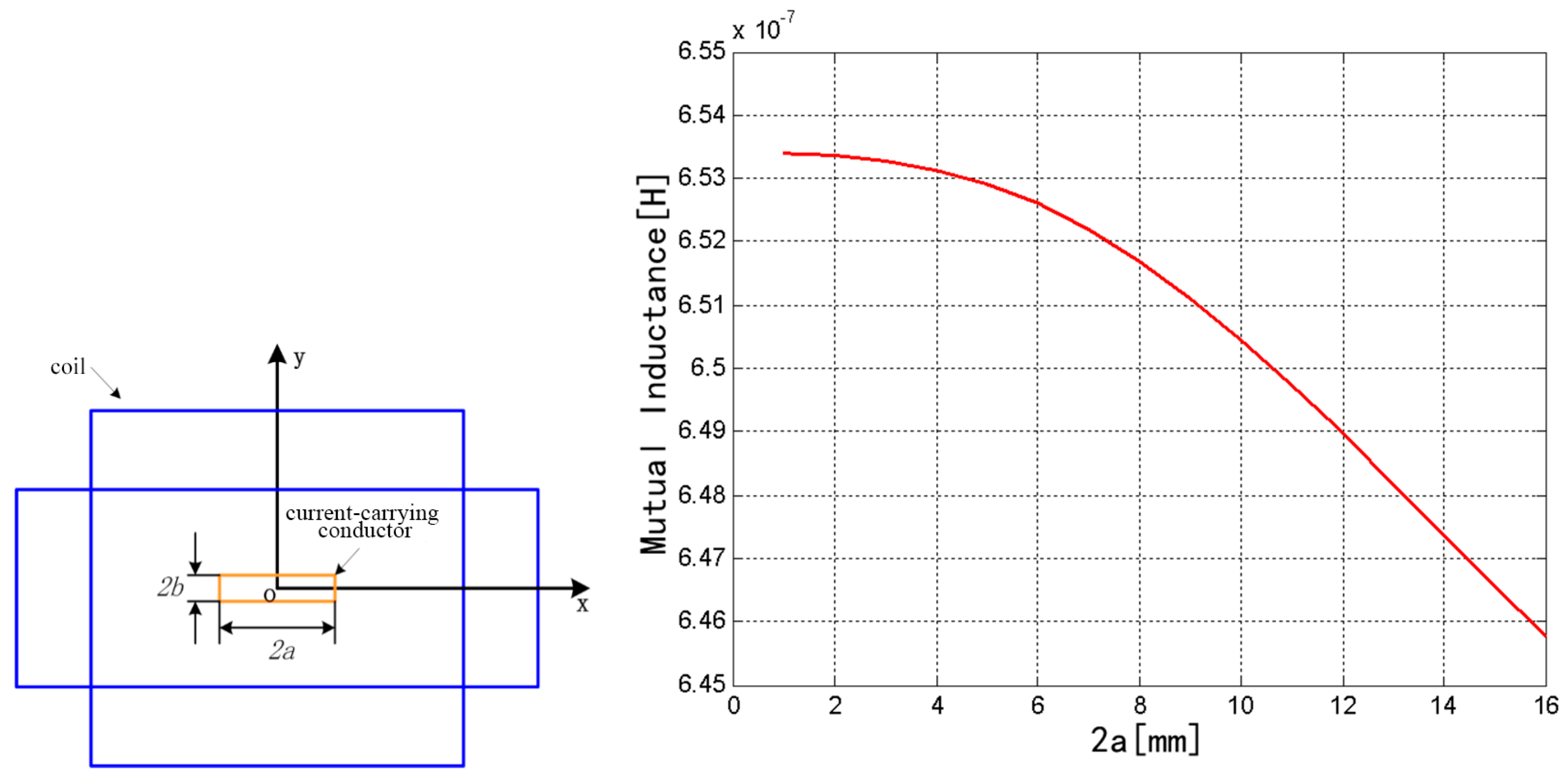
Figure 5.
Model of a rectangular conductor and a discrete RC, with 2a = 15 mm, 2b = 3 mm, c = 4 mm, h = 3 mm, L1 = 10 mm, L2 = 20 mm, d1 = 10 mm, d2 = 5 mm, ρ = 50 turns/mm.
Figure 5.
Model of a rectangular conductor and a discrete RC, with 2a = 15 mm, 2b = 3 mm, c = 4 mm, h = 3 mm, L1 = 10 mm, L2 = 20 mm, d1 = 10 mm, d2 = 5 mm, ρ = 50 turns/mm.
Figure 6.
Influence of rectangular conductor parameters on mutual inductance.
Figure 6.
Influence of rectangular conductor parameters on mutual inductance.
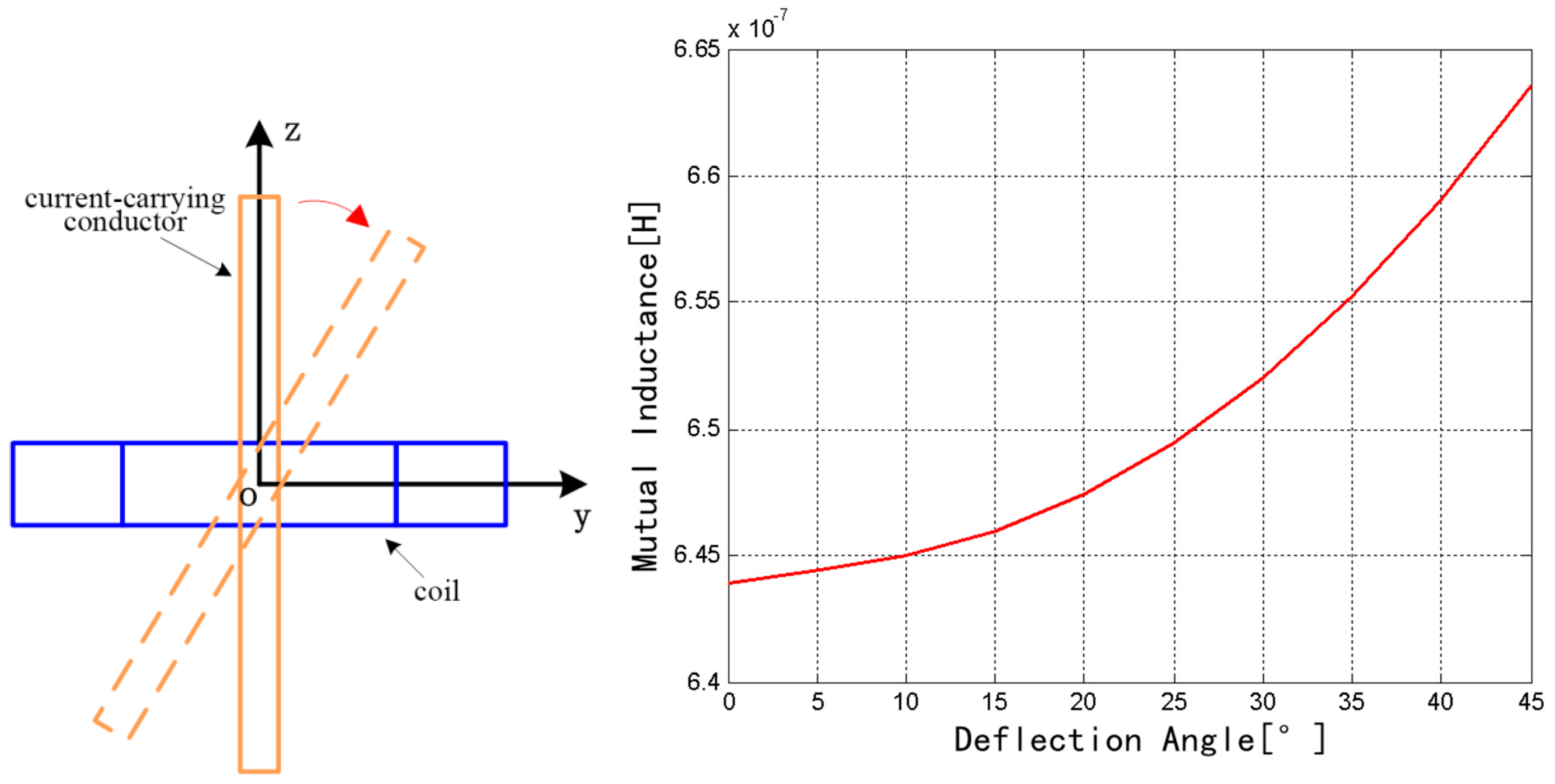
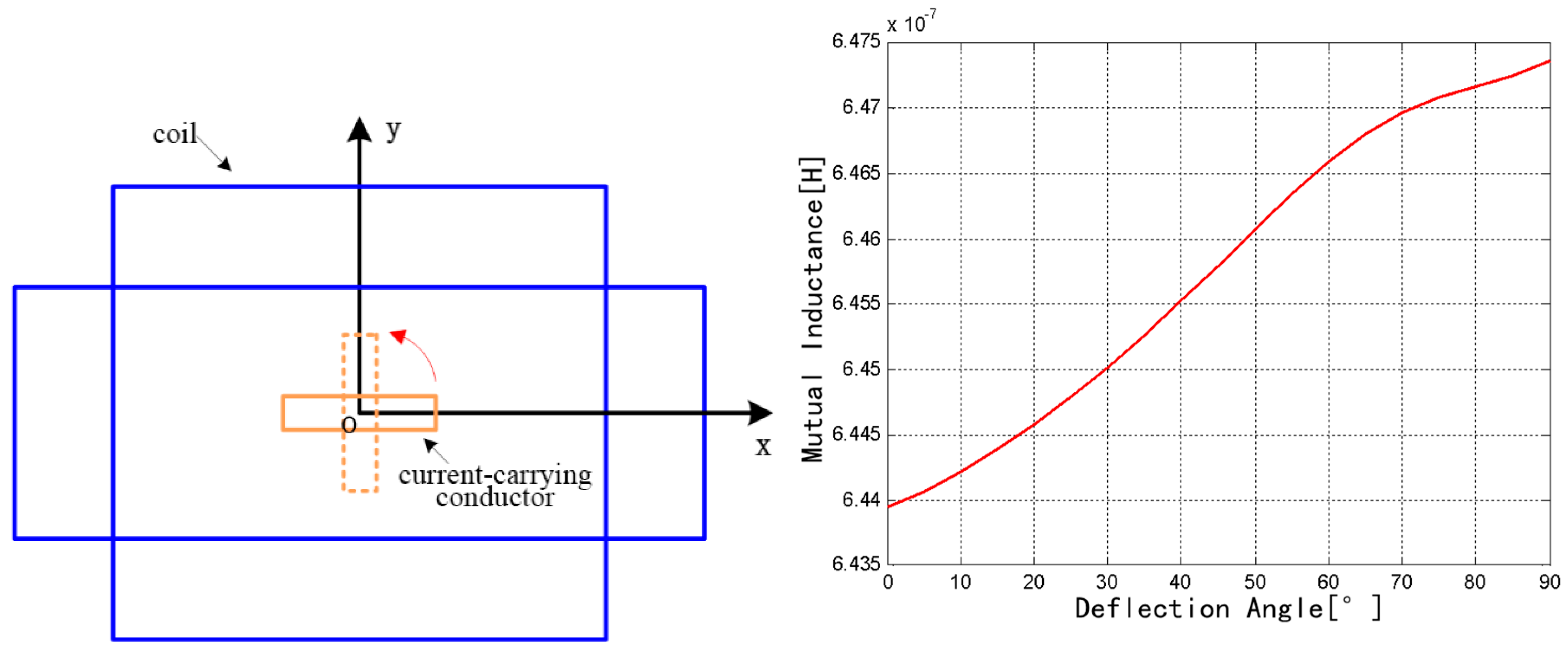
Figure 7.
Change of mutual inductance with the x axis as the rotation axis.
Figure 7.
Change of mutual inductance with the x axis as the rotation axis.
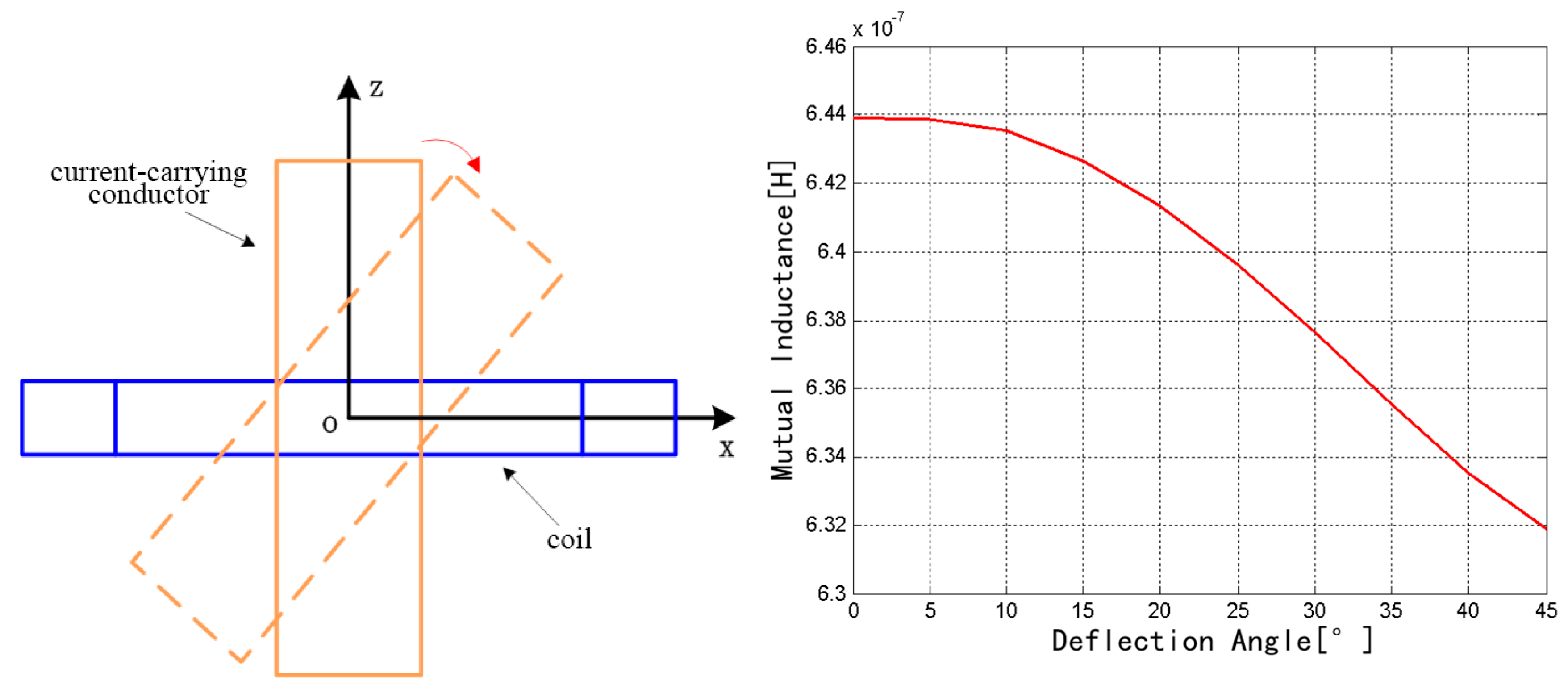
Figure 8.
Change of mutual inductance with the y axis as the rotation axis.
Figure 8.
Change of mutual inductance with the y axis as the rotation axis.
Figure 9.
Change of mutual inductance with the z axis as the rotation axis.
Figure 9.
Change of mutual inductance with the z axis as the rotation axis.
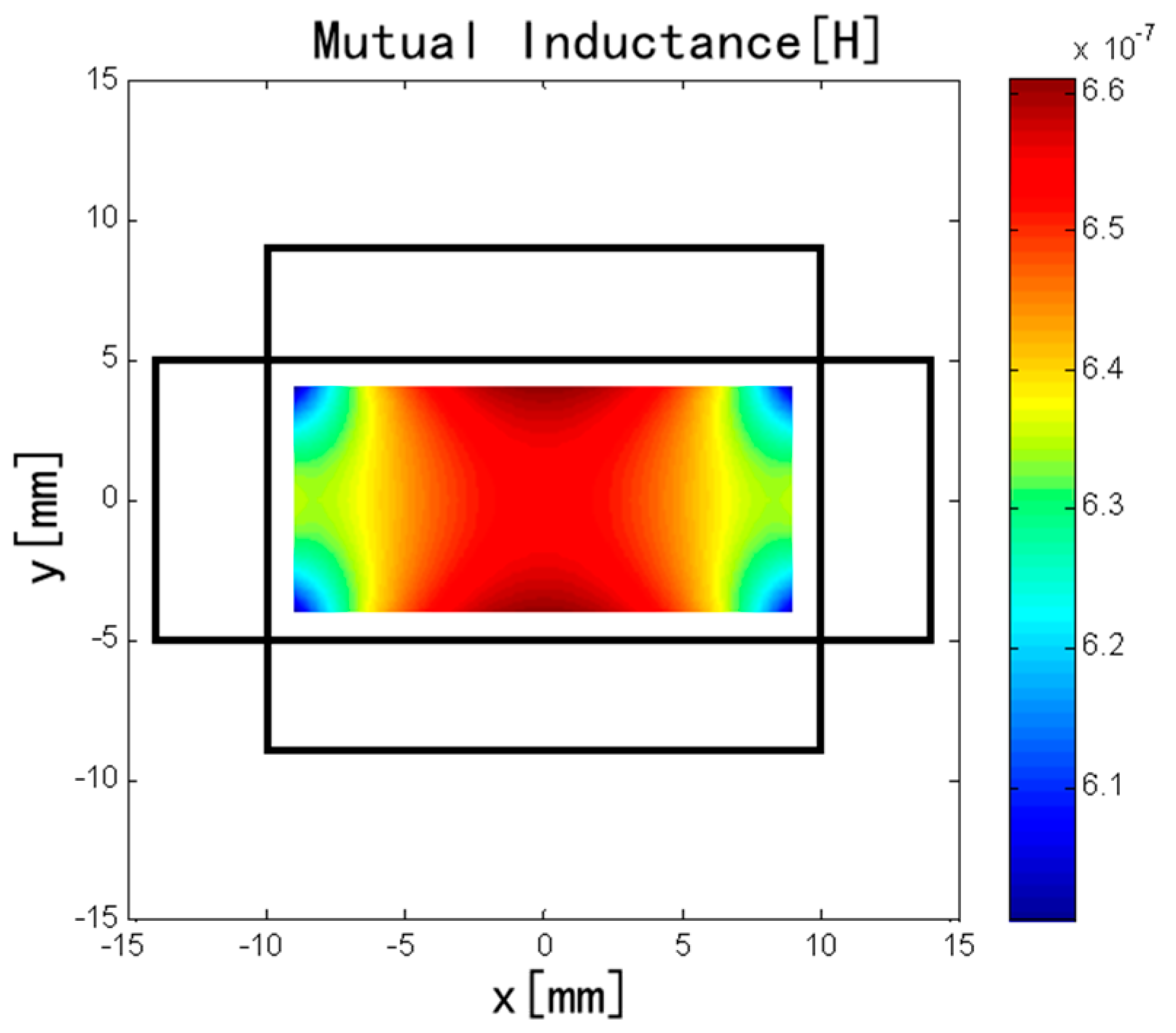
Figure 10.
Influence of eccentricity of the conductor on mutual inductance.
Figure 10.
Influence of eccentricity of the conductor on mutual inductance.
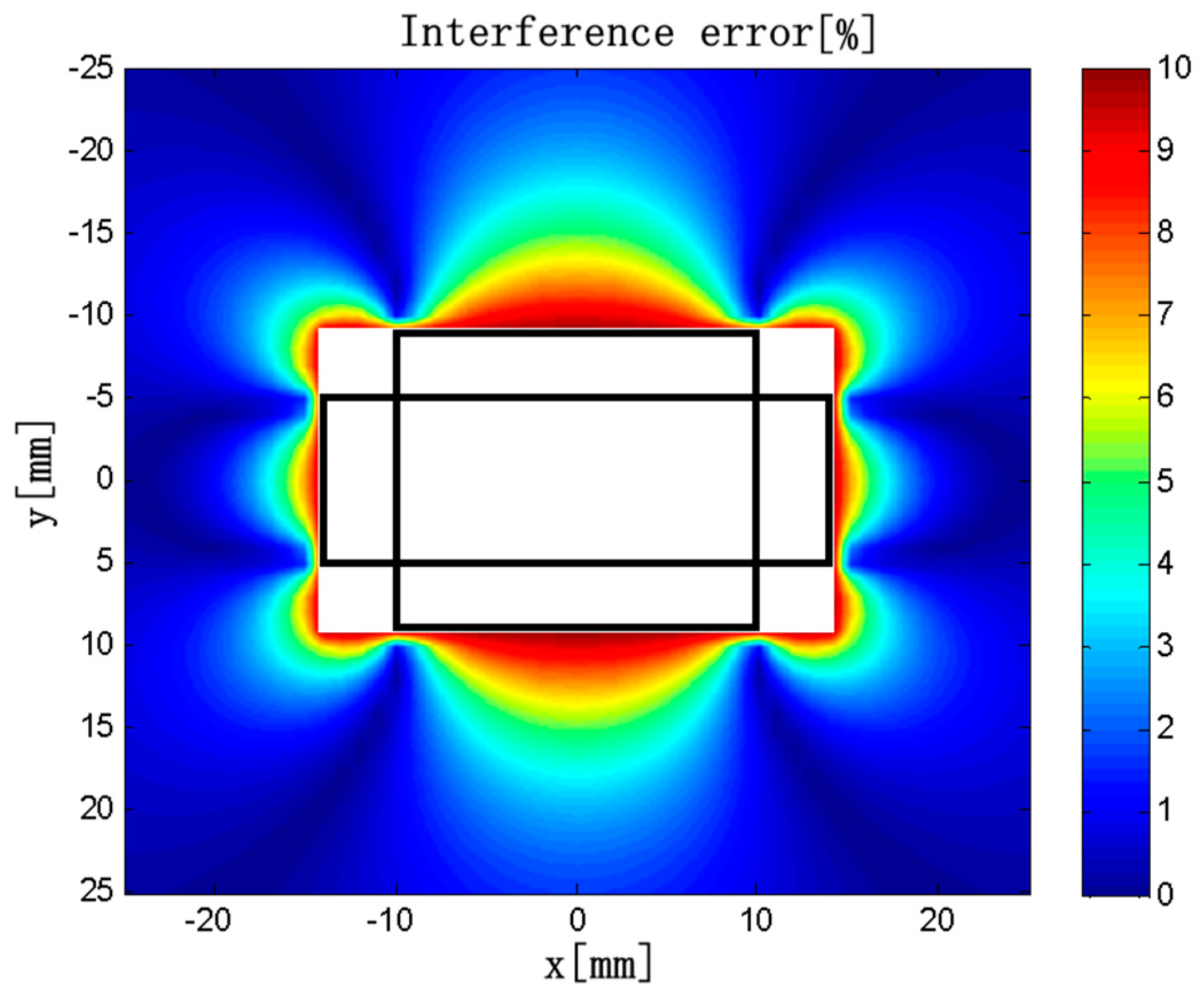
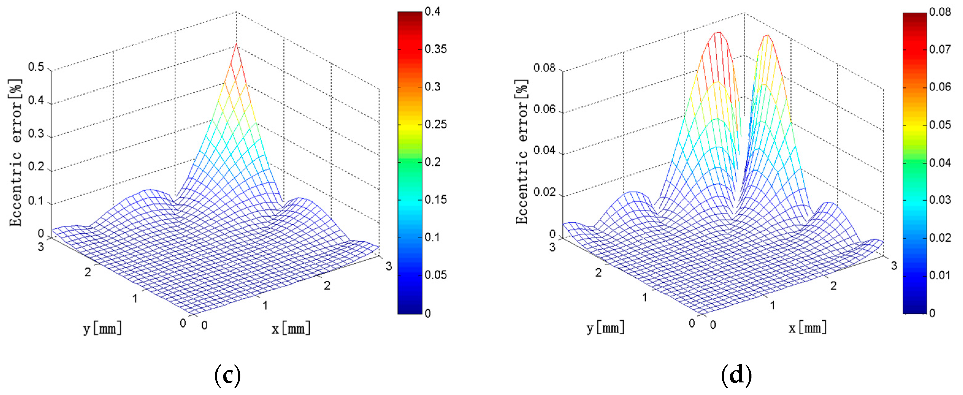
Figure 11.
Interference error distribution.
Figure 11.
Interference error distribution.
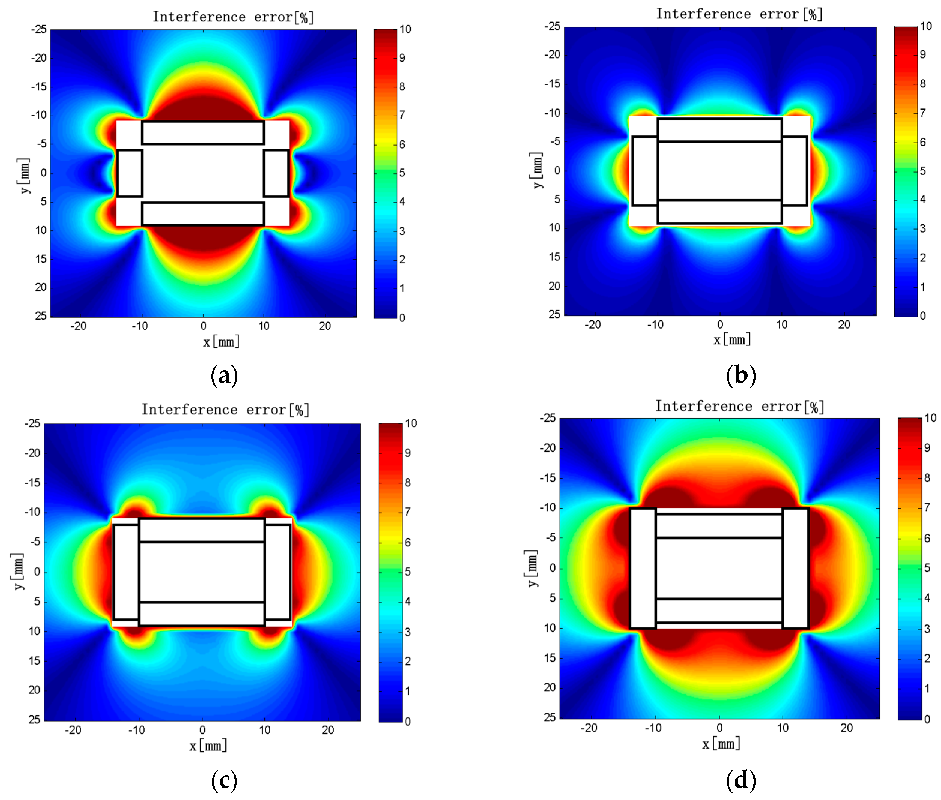
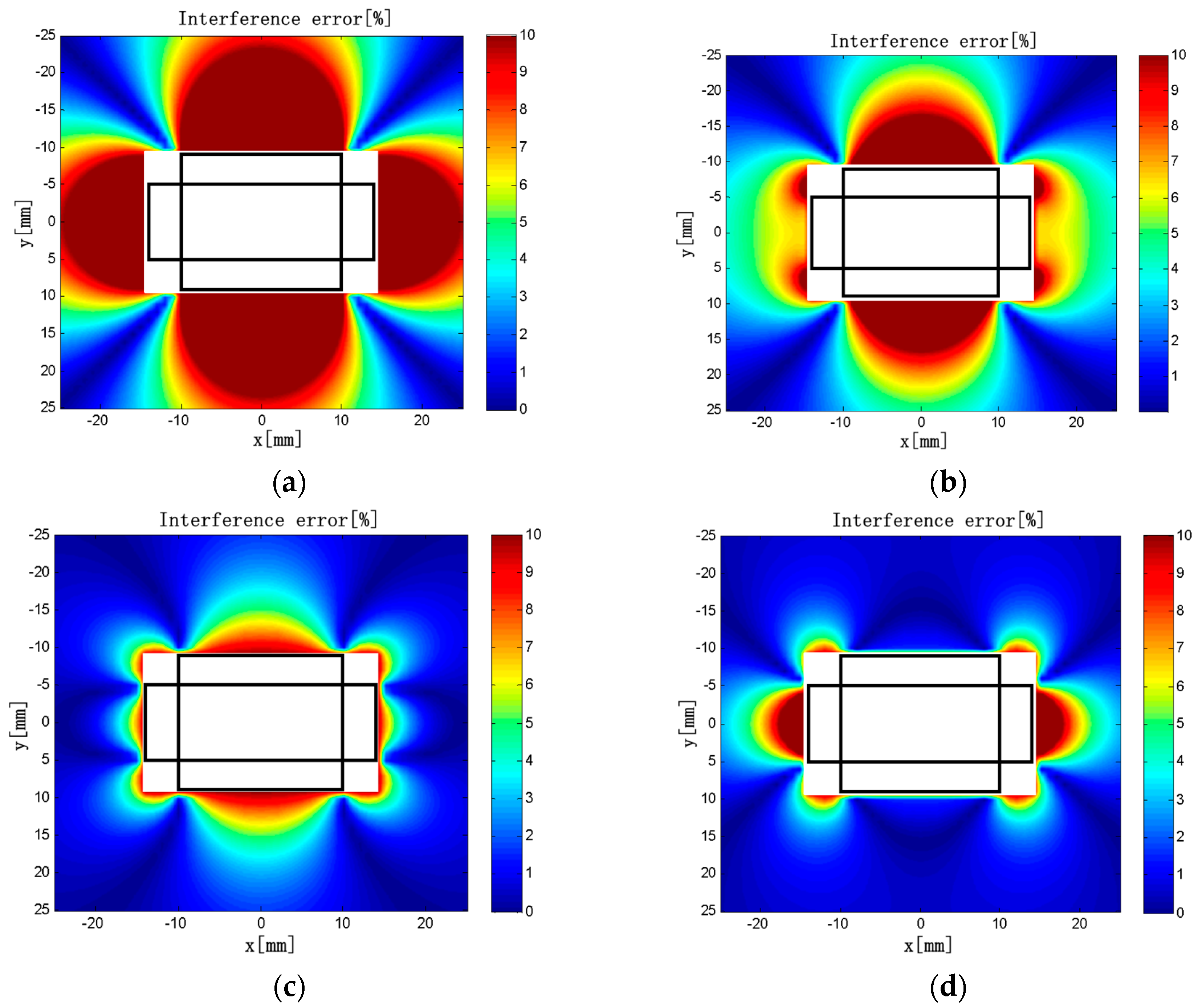
Figure 12.
(a) L1 = 8 mm; (b) L1 = 12 mm; (c) L1 = 16 mm; (d) L1 = 20 mm. Interference error distributions (L1 = 8–20 mm).
Figure 12.
(a) L1 = 8 mm; (b) L1 = 12 mm; (c) L1 = 16 mm; (d) L1 = 20 mm. Interference error distributions (L1 = 8–20 mm).
Figure 13.
(a) ρ1 = 10 turns/mm; (b) ρ1 = 30 turns/mm; (c) ρ1 = 50 turns/mm; (d) ρ1 = 70 turns/mm. Interference error distributions (ρ1 = 10–70 turns/mm).
Figure 13.
(a) ρ1 = 10 turns/mm; (b) ρ1 = 30 turns/mm; (c) ρ1 = 50 turns/mm; (d) ρ1 = 70 turns/mm. Interference error distributions (ρ1 = 10–70 turns/mm).
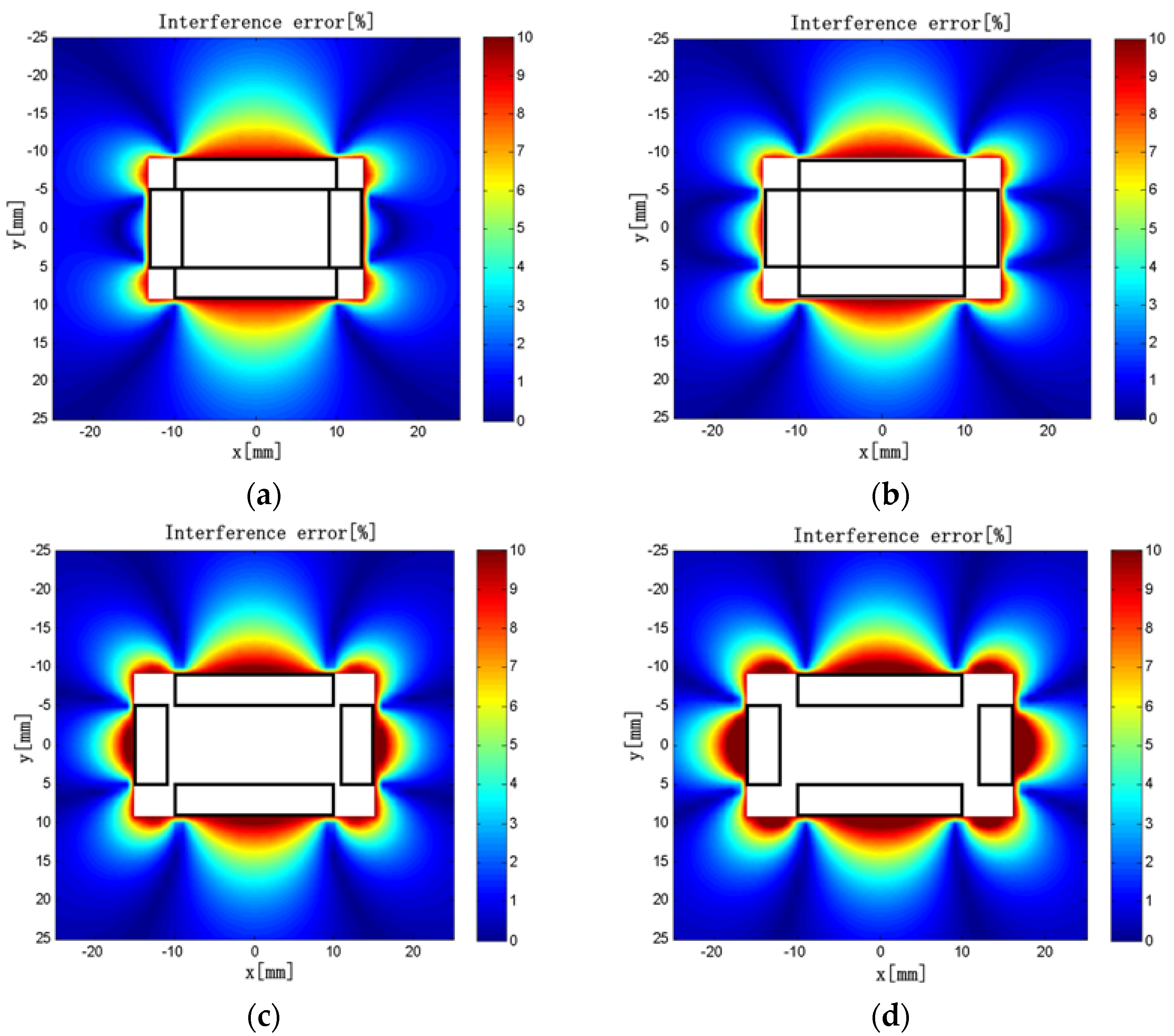
Figure 14.
(a) d1 = 9 mm; (b) d1 = 10 mm; (c) d1 = 11 mm; (d) d1 = 12 mm. Interference error distributions (d1 = 9–12 mm).
Figure 14.
(a) d1 = 9 mm; (b) d1 = 10 mm; (c) d1 = 11 mm; (d) d1 = 12 mm. Interference error distributions (d1 = 9–12 mm).
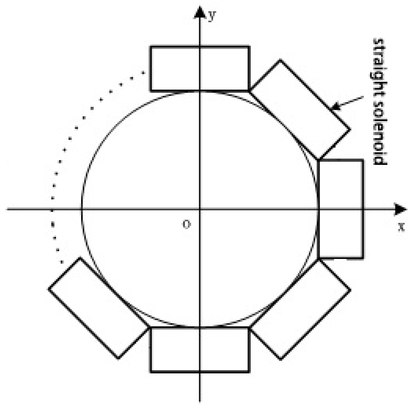
Figure 15.
A discrete RC of N solenoids.
Figure 15.
A discrete RC of N solenoids.
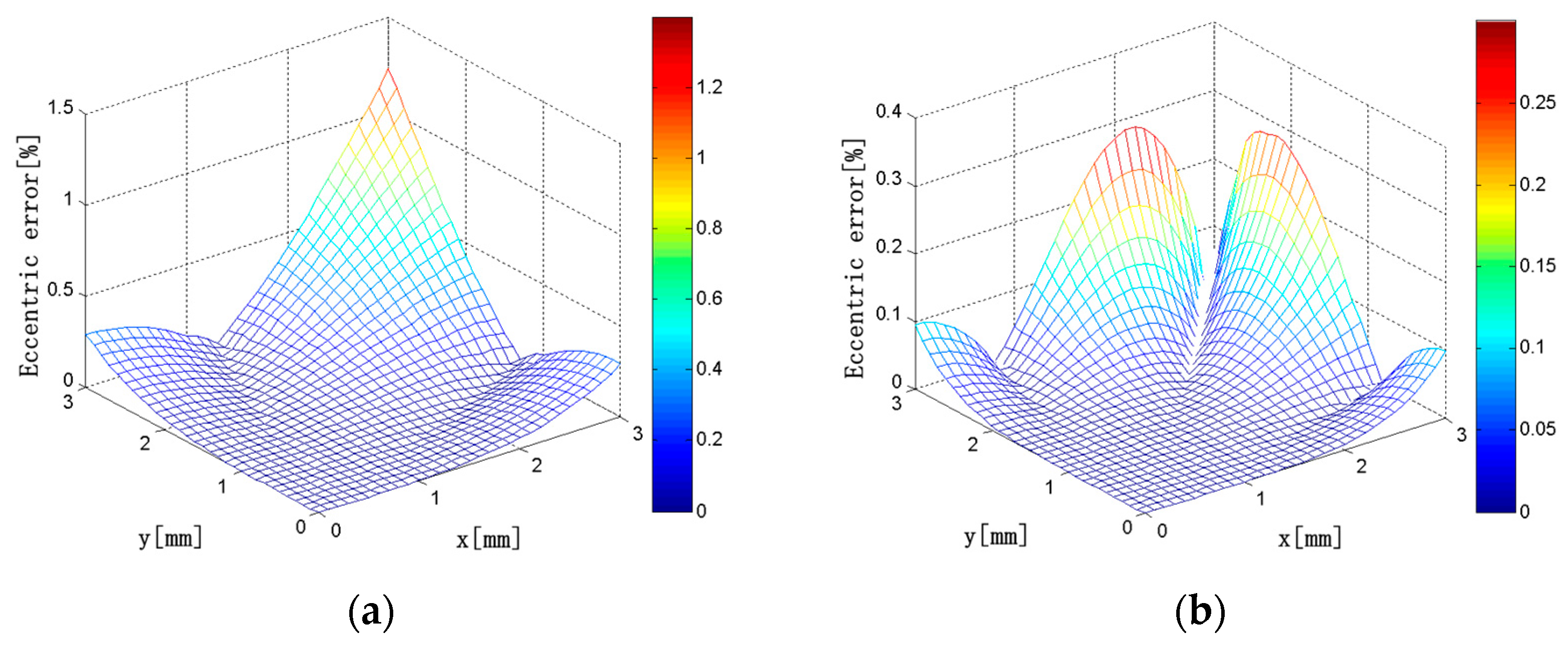
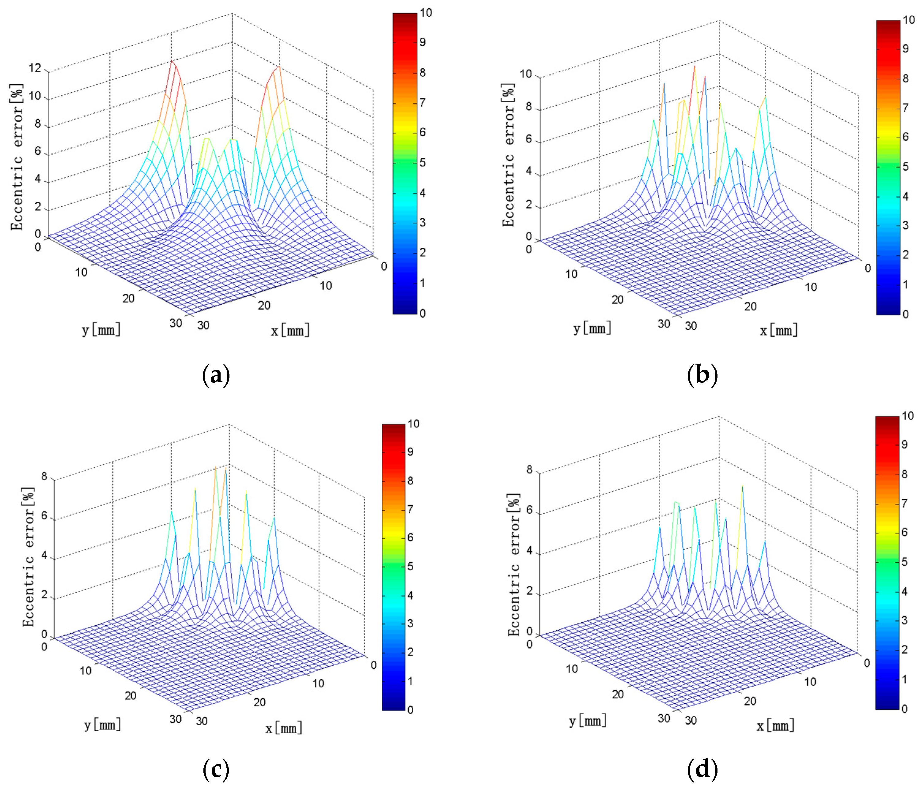
Figure 16.
(a) N = 4; (b) N = 6; (c) N = 8; (d) N = 10. Eccentricity error distributions (N = 4, 6, 8, 10; x = 0–3 mm; y = 0–3 mm).
Figure 16.
(a) N = 4; (b) N = 6; (c) N = 8; (d) N = 10. Eccentricity error distributions (N = 4, 6, 8, 10; x = 0–3 mm; y = 0–3 mm).
Figure 17.
(a) N = 4; (b) N = 6; (c) N = 8; (d) N = 10. Interference error distributions (N = 4, 6, 8, 10; x = 0–30 mm; y = 0–30 mm).
Figure 17.
(a) N = 4; (b) N = 6; (c) N = 8; (d) N = 10. Interference error distributions (N = 4, 6, 8, 10; x = 0–30 mm; y = 0–30 mm).
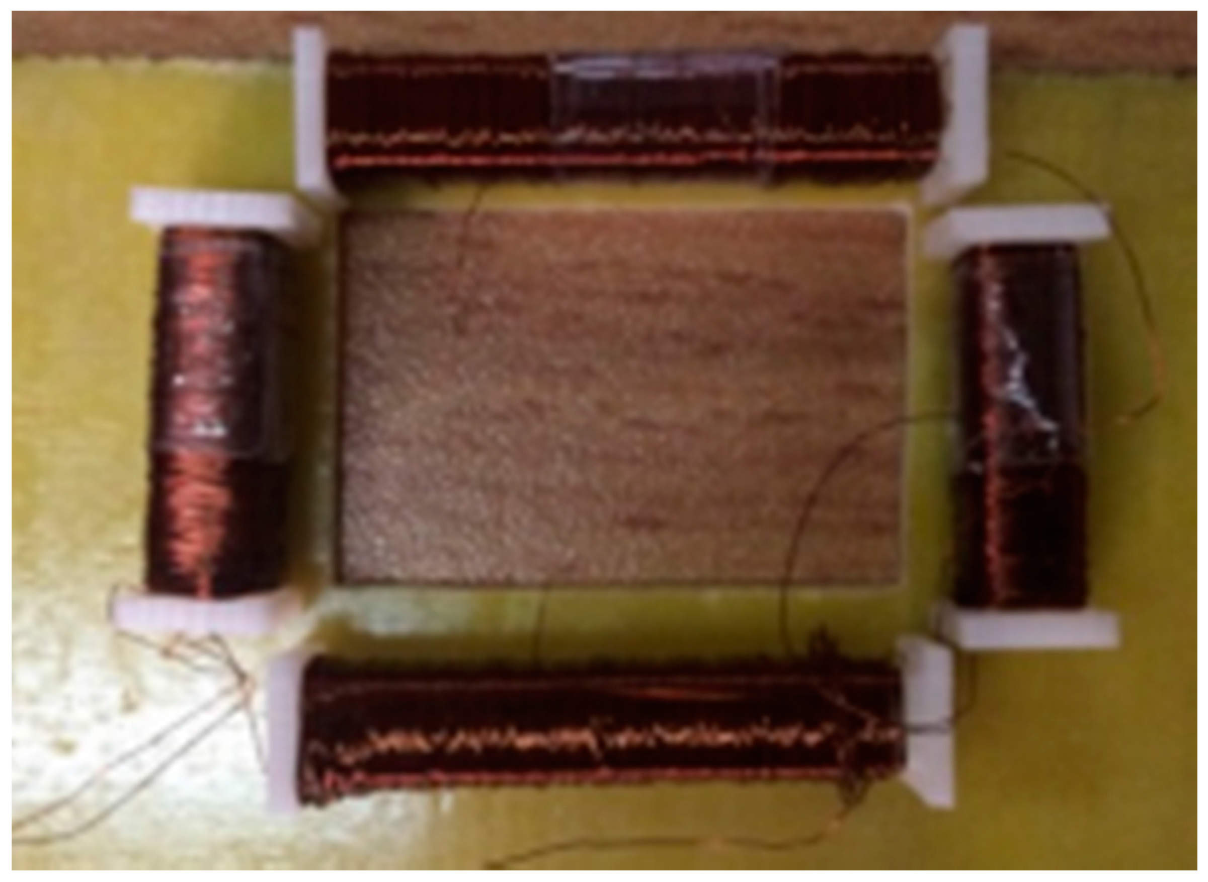
Figure 18.
Discrete RC prototype.
Figure 18.
Discrete RC prototype.
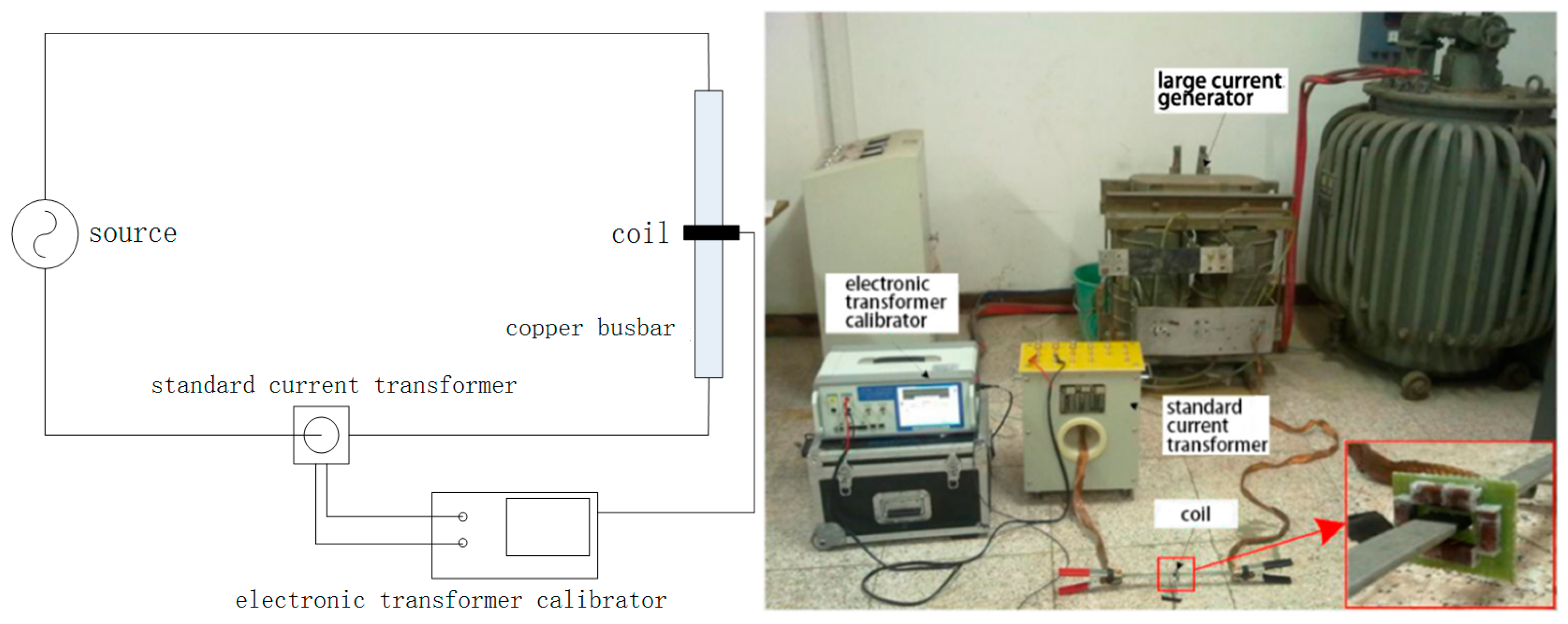
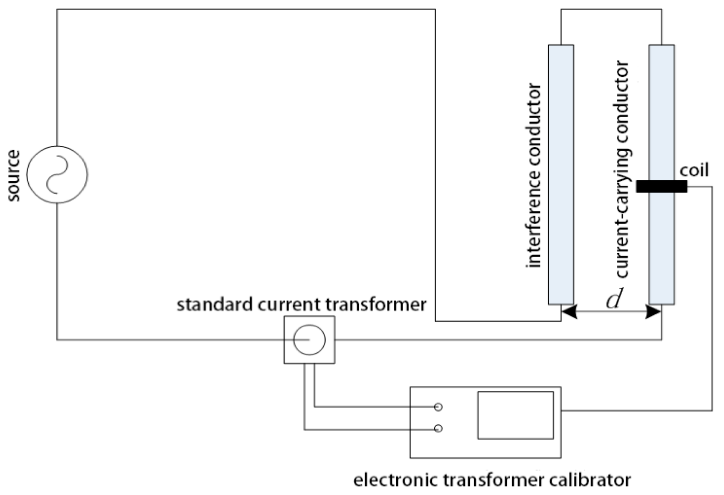
Figure 19.
Test circuit for a discrete RC.
Figure 19.
Test circuit for a discrete RC.
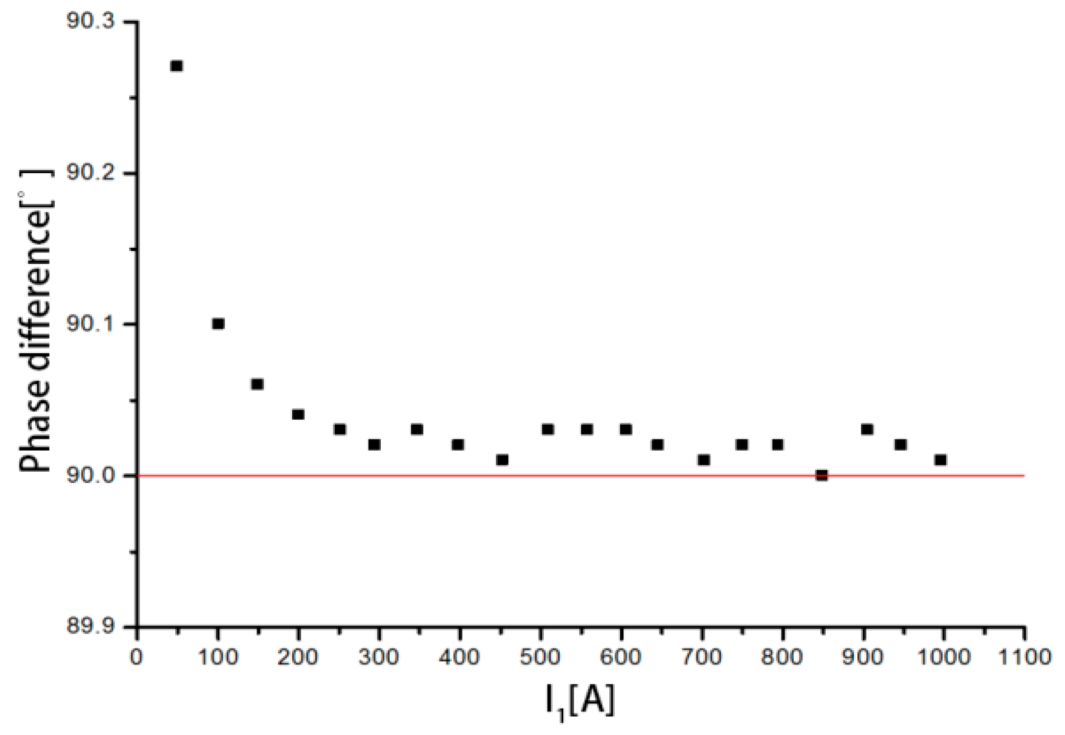
Figure 20.
Distribution of the phase difference.
Figure 20.
Distribution of the phase difference.
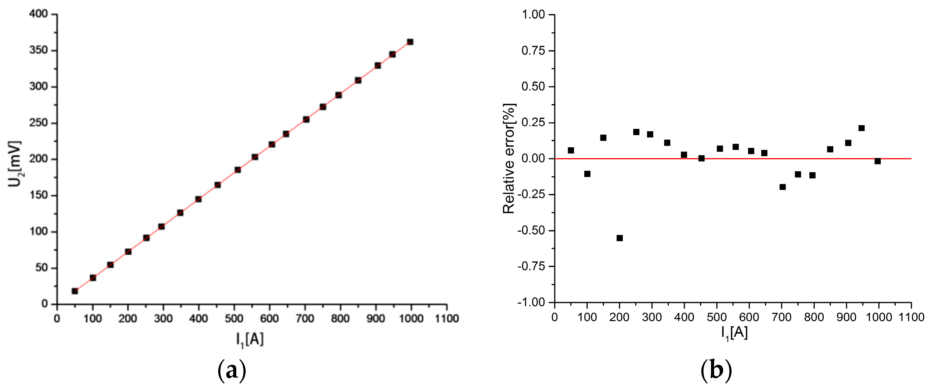
Figure 21.
(a) Relationship between the output voltage; (b) Relative error between the measured current and the measured current and the primary current. Out consistency of the discrete RC.
Figure 21.
(a) Relationship between the output voltage; (b) Relative error between the measured current and the measured current and the primary current. Out consistency of the discrete RC.
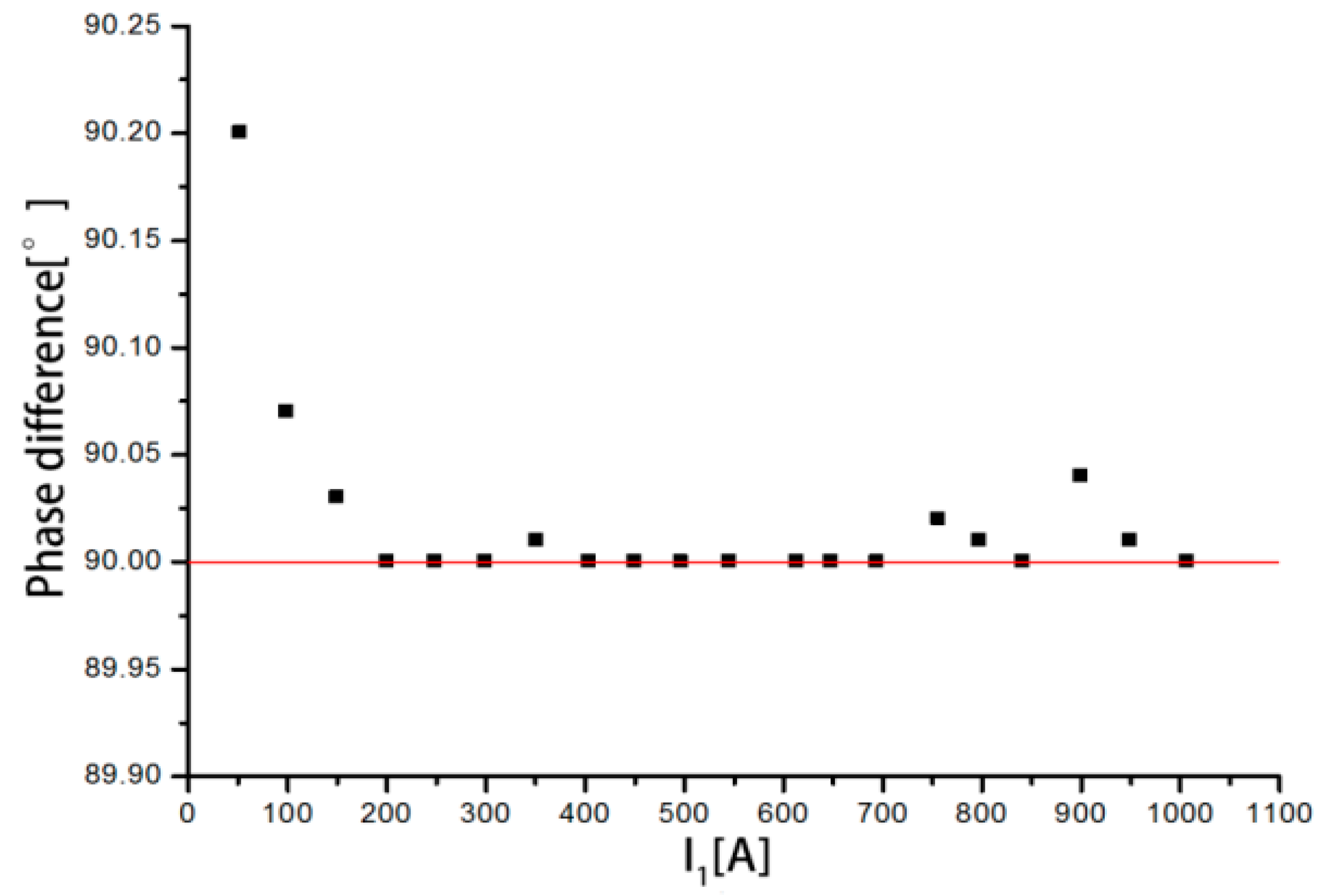
Figure 22.
Distribution of the phase difference.
Figure 22.
Distribution of the phase difference.
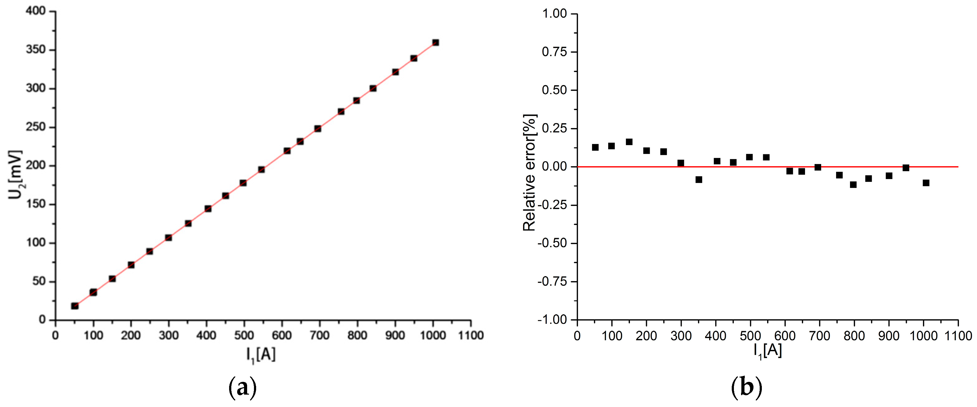
Figure 23.
(a) Relationship between the output voltage; (b) Relative error between the measured current and the measured current and the primary current. Out consistency of the discrete RC.
Figure 23.
(a) Relationship between the output voltage; (b) Relative error between the measured current and the measured current and the primary current. Out consistency of the discrete RC.
Table 1.
Mutual inductance of the circular conductor calculated by using the MVP method.
Table 1.
Mutual inductance of the circular conductor calculated by using the MVP method.
| Mutual Inductance | Rog1 | Rog2 | Rog3 | Rog4 | Rog |
|---|
| M [×10−7 H] | 0.9543 | 2.3142 | 0.9543 | 2.3143 | 6.5370 |
Table 2.
Mutual inductance of the circular conductor calculated by using the finite element method.
Table 2.
Mutual inductance of the circular conductor calculated by using the finite element method.
| Mutual Inductance | Rog1 | Rog2 | Rog3 | Rog4 | Rog |
|---|
| M [×10−7 H] | 0.9433 | 2.2863 | 0.9427 | 2.2880 | 6.4603 |
Table 3.
Mutual inductance of the rectangular conductor calculated by using the MVP method.
Table 3.
Mutual inductance of the rectangular conductor calculated by using the MVP method.
| Mutual Inductance | Rog1 | Rog2 | Rog3 | Rog4 | Rog |
|---|
| M [×10−7 H] | 1.0612 | 2.1715 | 1.0612 | 2.1715 | 6.4655 |
Table 4.
Mutual inductance of the rectangular conductor calculated by using the finite element method.
Table 4.
Mutual inductance of the rectangular conductor calculated by using the finite element method.
| Mutual Inductance | Rog1 | Rog2 | Rog3 | Rog4 | Rog |
|---|
| M [×10−7 H] | 1.0579 | 2.1355 | 1.0538 | 2.1398 | 6.3867 |
Table 5.
Maximum interference errors (L1 = 6–20 mm).
Table 5.
Maximum interference errors (L1 = 6–20 mm).
| L1 [mm] | 6 | 8 | 10 | 12 | 14 | 16 | 18 | 20 |
|---|
| Maximum interference error [%] | 19.1 | 13.9 | 9.3 | 8.5 | 10.0 | 11.0 | 15.4 | 16.2 |
Table 6.
Maximum interference errors (ρ1 = 10–80 turns/mm).
Table 6.
Maximum interference errors (ρ1 = 10–80 turns/mm).
| ρ1 [turns/mm] | 10 | 20 | 30 | 40 | 50 | 60 | 70 | 80 |
|---|
| Maximum interference error [%] | 32.7 | 25.4 | 19.2 | 13.9 | 9.3 | 12.8 | 17.7 | 22.1 |
Table 7.
Maximum interference errors (d1 = 8.5–12 mm).
Table 7.
Maximum interference errors (d1 = 8.5–12 mm).
| d1 [mm] | 8.5 | 9 | 9.5 | 10 | 10.5 | 11 | 11.5 | 12 |
|---|
| Maximum interference error [%] | 10.3 | 10.0 | 10.0 | 9.3 | 10.3 | 10.8 | 14.0 | 14.1 |
Table 8.
Experimental results using the discrete RC for measuring the circular conductor.
Table 8.
Experimental results using the discrete RC for measuring the circular conductor.
| Serial Number | Primary Current (RMS) I1 [A] | Secondary Voltage (RMS) U2 [mV] | Sensitivity S [mV·A−1] | Phase Difference [°] |
|---|
| 1 | 50.315 | 18.295 | 0.3636 | 90.27 |
| 2 | 101.018 | 36.671 | 0.3630 | 90.10 |
| 3 | 150.225 | 54.671 | 0.3639 | 90.06 |
| 4 | 200.965 | 72.628 | 0.3614 | 90.04 |
| 5 | 251.859 | 91.694 | 0.3641 | 90.03 |
| 6 | 294.777 | 107.302 | 0.3640 | 90.02 |
| 7 | 347.395 | 126.382 | 0.3638 | 90.03 |
| 8 | 399.021 | 145.043 | 0.3635 | 90.02 |
| 9 | 453.020 | 164.631 | 0.3634 | 90.01 |
| 10 | 509.943 | 185.440 | 0.3636 | 90.03 |
| 11 | 558.572 | 203.151 | 0.3637 | 90.03 |
| 12 | 606.185 | 220.404 | 0.3636 | 90.03 |
| 13 | 646.508 | 235.030 | 0.3635 | 90.02 |
| 14 | 703.246 | 255.056 | 0.3627 | 90.01 |
| 15 | 750.460 | 272.420 | 0.3630 | 90.02 |
| 16 | 794.924 | 288.540 | 0.3630 | 90.02 |
| 17 | 849.889 | 309.047 | 0.3636 | 90.01 |
| 18 | 905.480 | 329.408 | 0.3638 | 90.01 |
| 19 | 946.824 | 344.807 | 0.3642 | 90.02 |
| 20 | 996.523 | 362.075 | 0.3633 | 90.01 |
Table 9.
Results from the MVP method, the finite element method, and the experiment.
Table 9.
Results from the MVP method, the finite element method, and the experiment.
| | MVP Method | Finite Element Method | Experimental Result |
|---|
| Mutual inductance M [μH] | 1.0592 | 1.0496 | 1.1567 |
| Sensitivity S [mV·A−1] | 0.3328 | 0.3297 | 0.3634 |
Table 10.
Experimental results using the discrete RC for measuring the rectangular conductor.
Table 10.
Experimental results using the discrete RC for measuring the rectangular conductor.
| Serial Number | Primary Current (RMS) I1 [A] | Secondary Voltage (RMS) U2 [mV] | Sensitivity S [mV·A−1] | Phase Difference [°] |
|---|
| 1 | 52.340 | 18.725 | 0.3577 | 90.20 |
| 2 | 99.137 | 35.470 | 0.3578 | 90.07 |
| 3 | 150.121 | 53.726 | 0.3579 | 90.03 |
| 4 | 200.232 | 71.619 | 0.3577 | 90.01 |
| 5 | 249.176 | 89.119 | 0.3577 | 90.00 |
| 6 | 299.091 | 106.892 | 0.3574 | 90.00 |
| 7 | 351.436 | 125.463 | 0.3570 | 90.01 |
| 8 | 403.993 | 144.400 | 0.3574 | 89.99 |
| 9 | 450.590 | 161.040 | 0.3574 | 90.00 |
| 10 | 496.993 | 177.687 | 0.3575 | 90.00 |
| 11 | 545.776 | 195.127 | 0.3575 | 90.00 |
| 12 | 613.740 | 219.226 | 0.3572 | 90.00 |
| 13 | 648.250 | 231.547 | 0.3572 | 90.00 |
| 14 | 694.619 | 248.179 | 0.3573 | 90.02 |
| 15 | 756.817 | 270.262 | 0.3571 | 90.01 |
| 16 | 797.323 | 284.550 | 0.3569 | 89.99 |
| 17 | 841.110 | 300.296 | 0.3570 | 90.03 |
| 18 | 900.568 | 321.584 | 0.3571 | 90.01 |
| 19 | 949.103 | 339.091 | 0.3573 | 90.00 |
| 20 | 1007.370 | 359.554 | 0.3569 | 90.00 |
Table 11.
Results from the MVP method, the finite element method, and the experiment.
Table 11.
Results from the MVP method, the finite element method, and the experiment.
| | MVP Method | Finite Element Method | Experimental Value |
|---|
| Mutual inductance M [μH] | 1.0510 | 1.0410 | 1.1373 |
| Sensitivity S [mV·A−1] | 0.3302 | 0.3270 | 0.3573 |
Table 12.
Experimental results (d = 45 mm).
Table 12.
Experimental results (d = 45 mm).
| Serial Number | Primary Current (RMS) I1 [A] | Secondary Voltage (RMS) U2 [mV] | Interference Error [%] |
|---|
| 1 | 98.579 | 35.573 | 1.0 |
| 2 | 202.633 | 73.074 | 0.9 |
| 3 | 293.964 | 107.186 | 1.0 |
| 4 | 394.972 | 142.250 | 0.8 |
| 5 | 506.316 | 182.450 | 0.8 |
| 6 | 601.667 | 216.804 | 0.8 |
| 7 | 702.007 | 252.957 | 0.8 |
| 8 | 798.385 | 287.733 | 0.9 |
| 9 | 902.281 | 325.729 | 1.0 |
| 10 | 1000.160 | 360.959 | 1.0 |
Table 13.
Experimental results (d = 75 mm).
Table 13.
Experimental results (d = 75 mm).
| Serial Number | Primary Current (RMS) I1 [A] | Secondary Voltage (RMS) U2 [mV] | Interference Error [%] |
|---|
| 1 | 99.189 | 35.639 | 0.6 |
| 2 | 193.137 | 69.365 | 0.5 |
| 3 | 299.396 | 107.593 | 0.6 |
| 4 | 397.752 | 142.981 | 0.6 |
| 5 | 498.513 | 179.303 | 0.7 |
| 6 | 603.003 | 217.001 | 0.7 |
| 7 | 703.761 | 253.194 | 0.7 |
| 8 | 799.491 | 287.661 | 0.7 |
| 9 | 899.589 | 323.168 | 0.5 |
| 10 | 993.415 | 356.939 | 0.6 |


