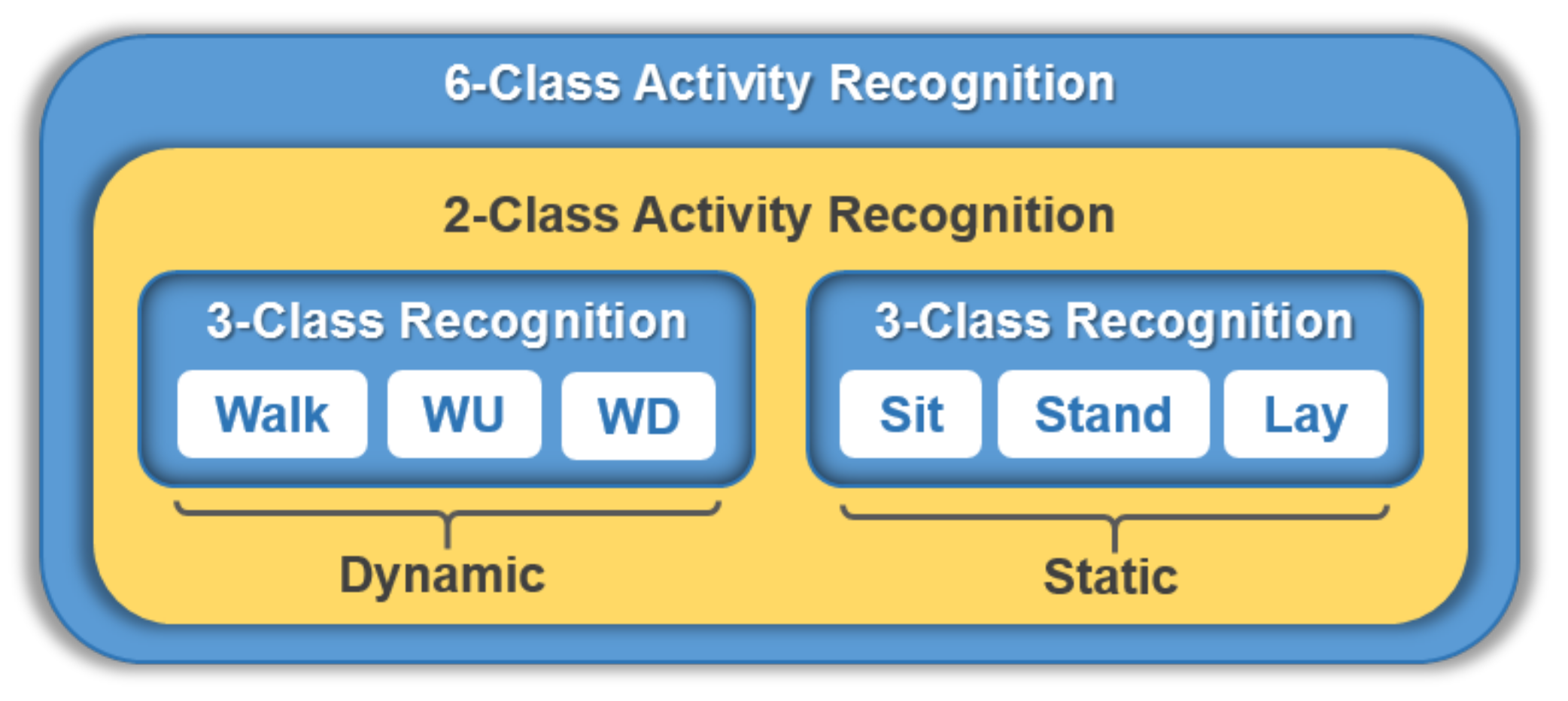
Figure 1.
Division of 6-class HAR into two-stage n-class HAR. Six activities, i.e., Walk, WU (Walk Upstairs), WD (Walk Downstairs), Sit, Stand, and Lay, are divided into two groups of abstract activities, Dynamic and Static, to form a 2-class HAR. Each abstract activity forms a 3-class HAR.
Figure 1.
Division of 6-class HAR into two-stage n-class HAR. Six activities, i.e., Walk, WU (Walk Upstairs), WD (Walk Downstairs), Sit, Stand, and Lay, are divided into two groups of abstract activities, Dynamic and Static, to form a 2-class HAR. Each abstract activity forms a 3-class HAR.
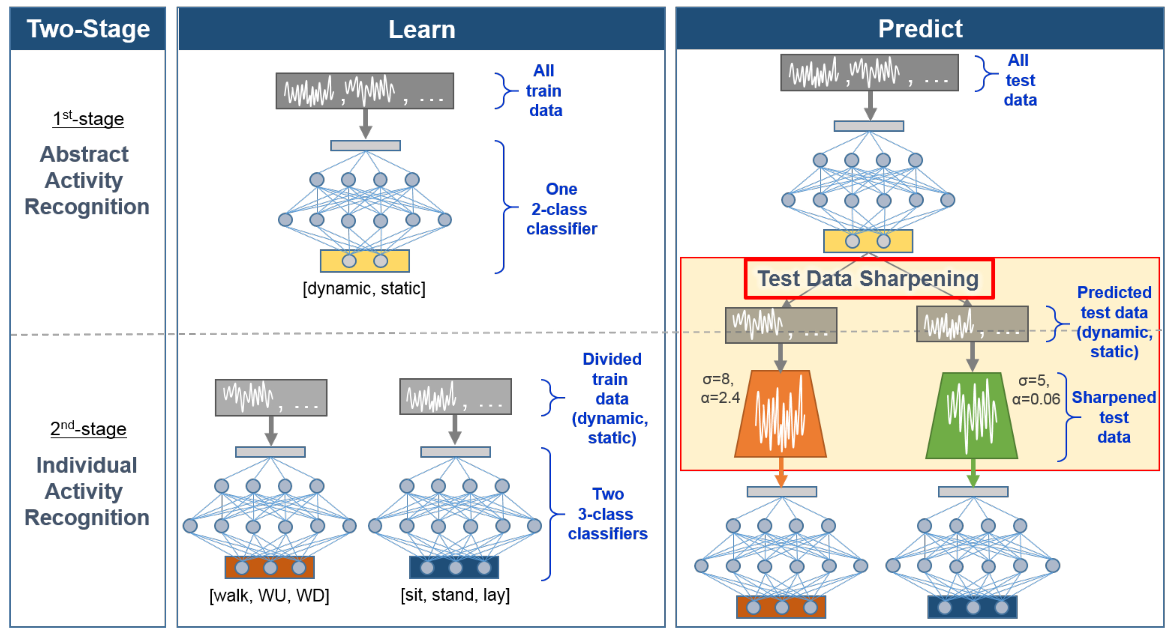
Figure 2.
Overview of our divide and conquer-based 1D CNN HAR with test data sharpening. Our approach employs two-stage classifier learning during the learning phase and introduces test data sharpening during the prediction phase.
Figure 2.
Overview of our divide and conquer-based 1D CNN HAR with test data sharpening. Our approach employs two-stage classifier learning during the learning phase and introduces test data sharpening during the prediction phase.
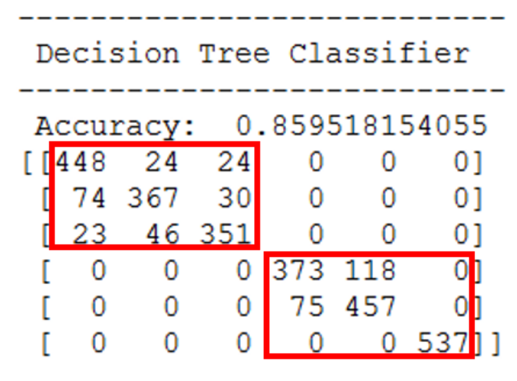
Figure 3.
Confusion matrix of decision tree classifier on 6-class HAR. For some pairwise activity classes, there are no misclassified instances as indicated by the positions with zeros in the confusion matrix.
Figure 3.
Confusion matrix of decision tree classifier on 6-class HAR. For some pairwise activity classes, there are no misclassified instances as indicated by the positions with zeros in the confusion matrix.
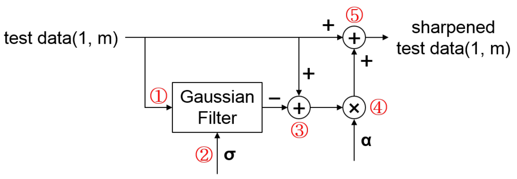
Figure 4.
Test data sharpening using a Gaussian filter. Test data is first denoised using a Gaussian filter (①) using the parameter (②), and the denoised result is subtracted from the test data to obtain sharped details (③). The sharpened details are then amplified to some degree using parameter (④) and added to the original test data to obtain sharpened test data (⑤).
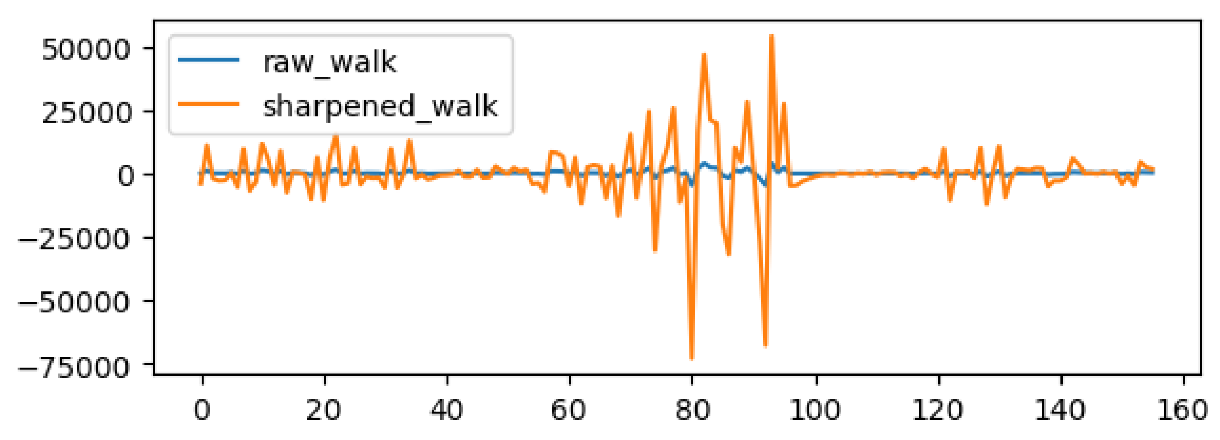
Figure 5.
A sample activity data describing walking activity. Each number in the horizontal axis indicates various statistical features such as mean, standard deviation, minimum and maximum calculated from a fixed length time series data collected from multiple sensors. The blue line indicates data before sharpening and the orange line indicates data after sharpening.
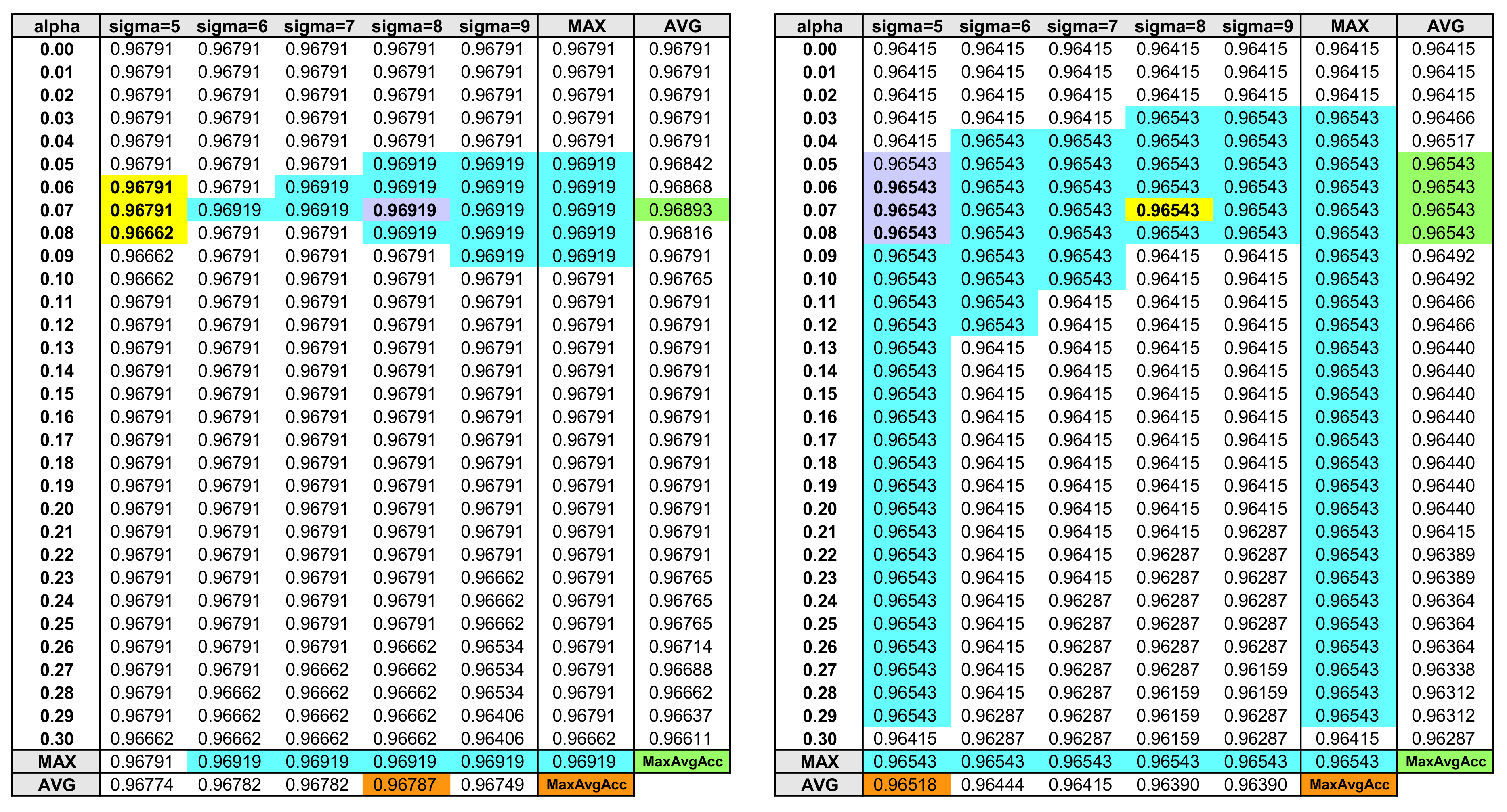
Figure 6.
Validation/test data HAR accuracy using different (, ) combinations. The cyan colored cells indicate the highest activity recognition accuracy. Maximum of average accuracy (MaxAvgAcc) is searched for various average accuracies of and values in order to find the suitable (, ) parameter values (orange and green colored cells). Assuming that the left table is the HAR accuracy of validation data, the purple cell where the two MaxAvgAccs meet identifies the suitable values ( = 8, = 0.07). Assuming that the right table is the HAR accuracy of test data, the yellow cell at ( = 8, = 0.07) achieves the highest accuracy of 96.543%.
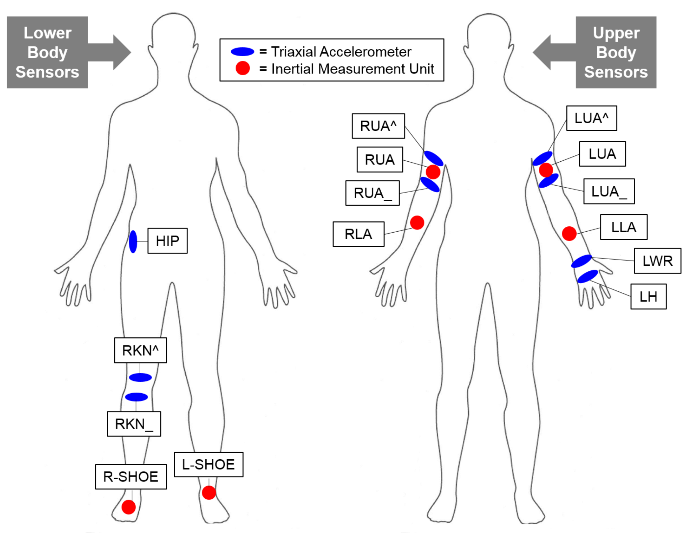
Figure 7.
Lower (left) and upper (right) body sensors selected for OPPORTUNITY dataset experiment. For the lower body sensors, we chose three triaxial accelerometers (marked in blue) located at the right hip (HIP), right knee (RKN^), and right knee (RKN_), and three inertial measurement units (marked in red) located at the right (R-SHOE) and left shoe (L-SHOE) for the experiments. For the upper body sensors, we chose six triaxial accelerometers located at the right upper arm (RUA^), right upper arm (RUA_), left upper arm (LUA^), left upper arm (LUA_), left wrist (LWR), and left hand (LH), and four inertial measurement units located at the right upper arm (RUA), right lower arm (RLA), left upper arm (LUA), and left lower arm (LLA).
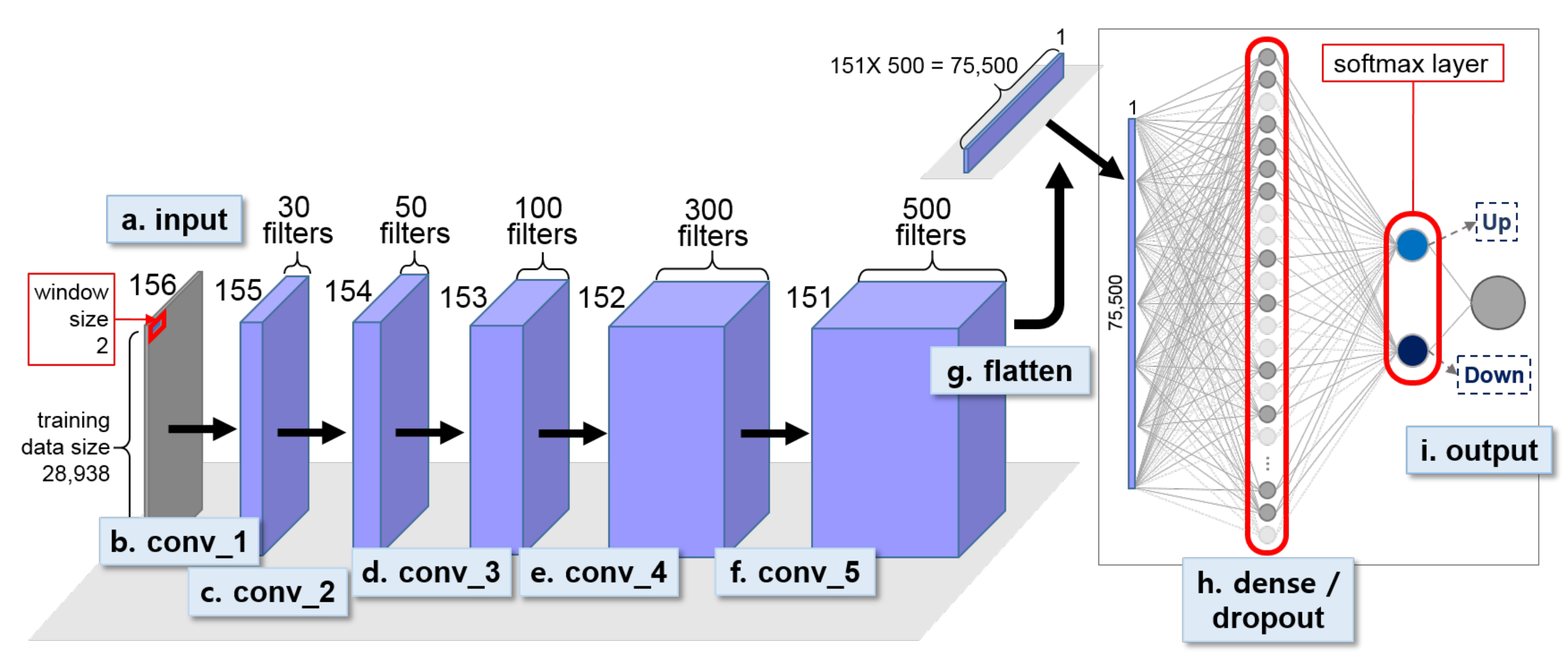
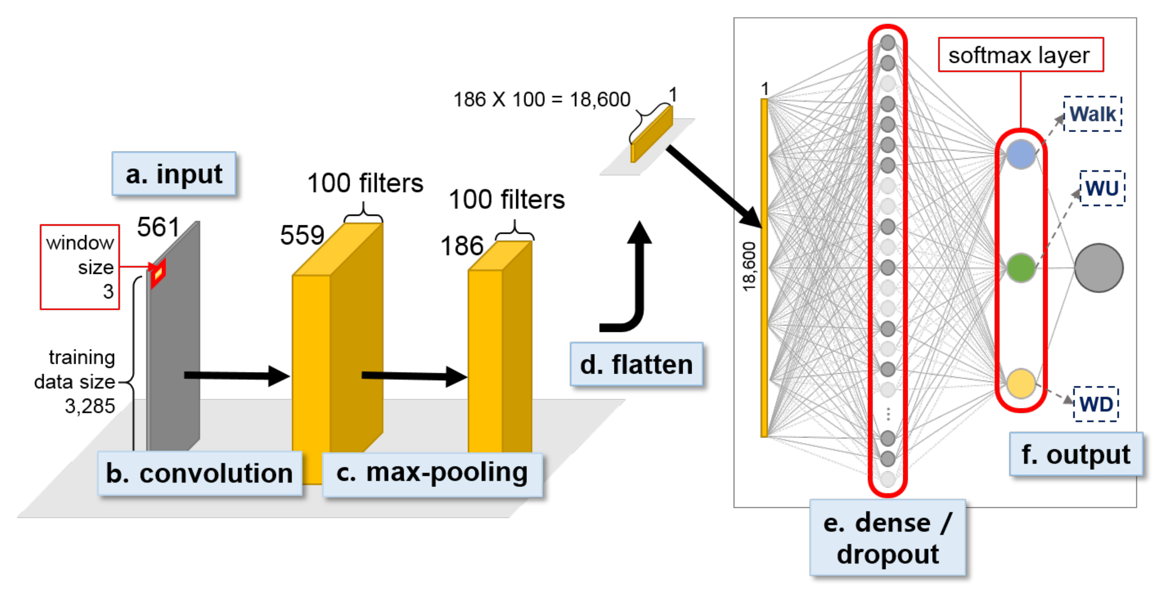
Figure 8.
First-stage 1D CNN for classifying abstract activities, i.e., Up and Down, for OPPORTUNITY dataset.
Figure 8.
First-stage 1D CNN for classifying abstract activities, i.e., Up and Down, for OPPORTUNITY dataset.
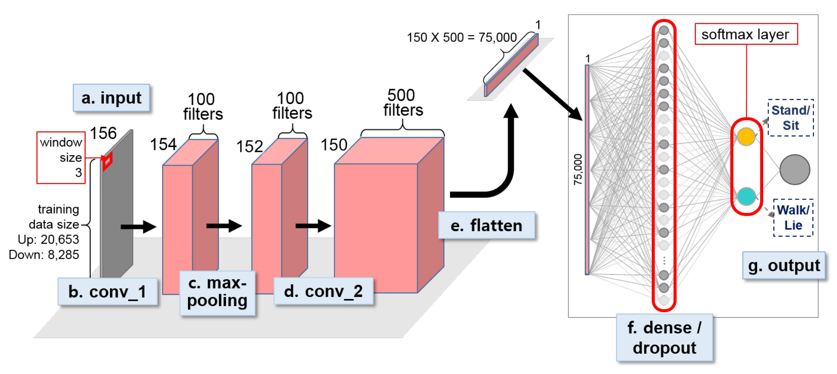
Figure 9.
Second-stage 1D CNN for classifying individual activities for OPPORTUNITY dataset. Two identically designed 1D CNNs were constructed to distinguish Stand from Walk and Sit from Lie.
Figure 9.
Second-stage 1D CNN for classifying individual activities for OPPORTUNITY dataset. Two identically designed 1D CNNs were constructed to distinguish Stand from Walk and Sit from Lie.
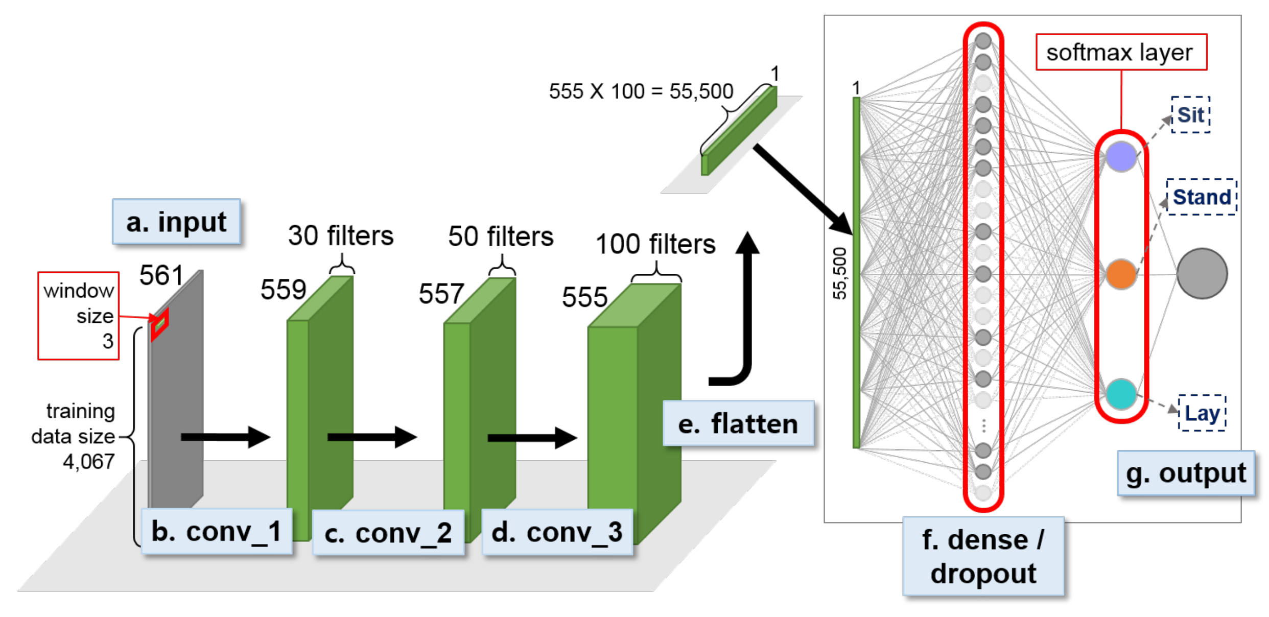
Figure 10.
Second-stage 1D CNN for classifying dynamic activity, i.e., Walk, WU, and WD, for UCI HAR dataset.
Figure 10.
Second-stage 1D CNN for classifying dynamic activity, i.e., Walk, WU, and WD, for UCI HAR dataset.
Figure 11.
Second-stage 1D CNN for classifying static acitivity, i.e., Sit, Stand, and Lay, for UCI HAR dataset.
Figure 11.
Second-stage 1D CNN for classifying static acitivity, i.e., Sit, Stand, and Lay, for UCI HAR dataset.
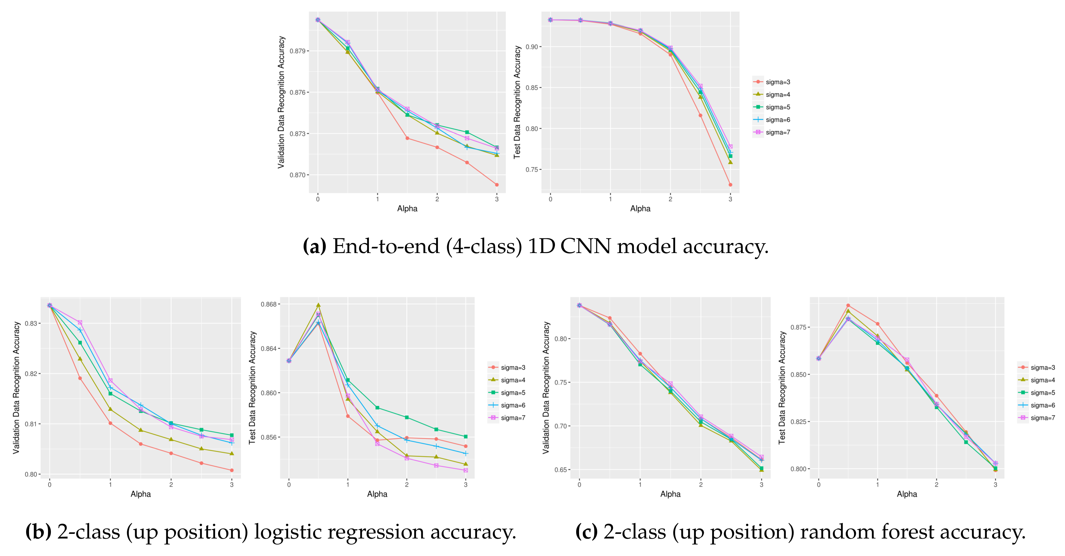
Figure 12.
Stand vs. walk recognition accuracy using different (, ) combinations on lower body OPPORTUNITY dataset (left: validation data, right: test data).
Figure 12.
Stand vs. walk recognition accuracy using different (, ) combinations on lower body OPPORTUNITY dataset (left: validation data, right: test data).
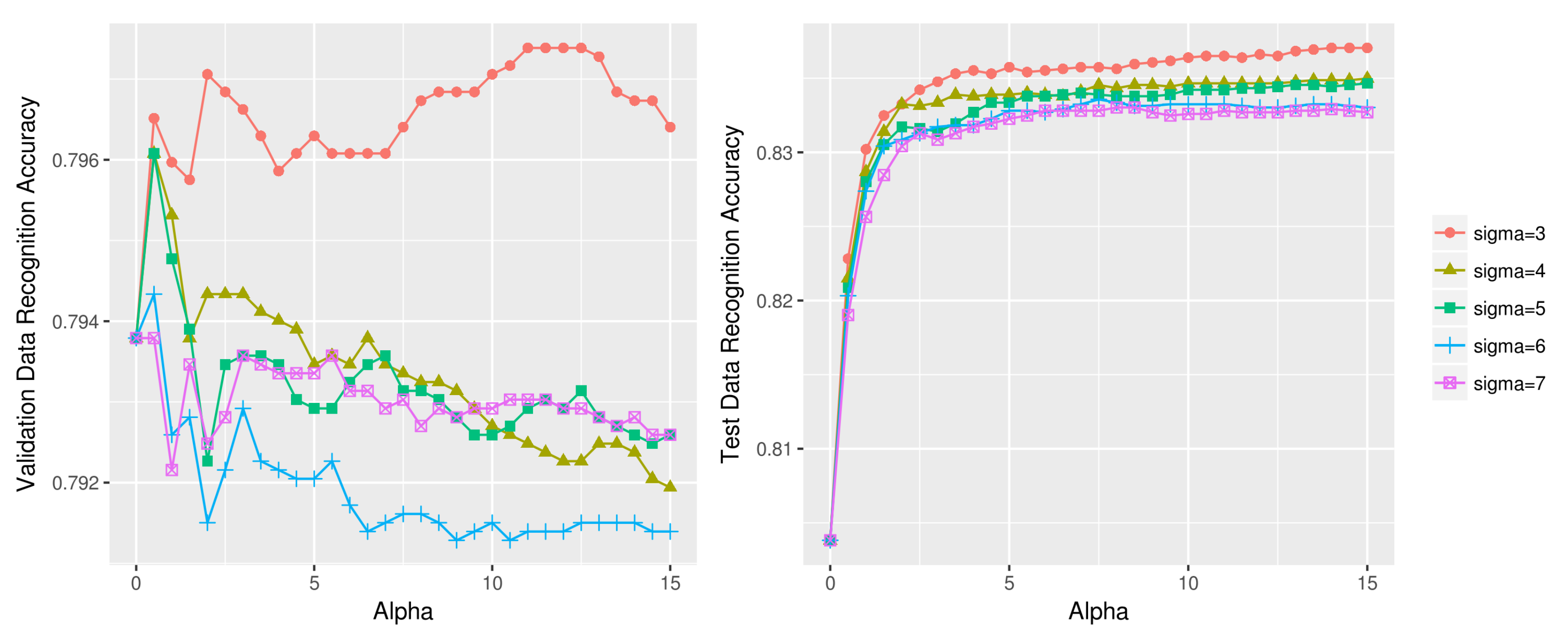
Figure 13.
Stand vs. walk recognition accuracy using different (, ) combinations on upper body OPPORTUNITY dataset (left: validation data, right: test data).
Figure 13.
Stand vs. walk recognition accuracy using different (, ) combinations on upper body OPPORTUNITY dataset (left: validation data, right: test data).
Figure 14.
Unsuccessful test data sharpening cases using lower body data (left: validation, right: test).
Figure 14.
Unsuccessful test data sharpening cases using lower body data (left: validation, right: test).
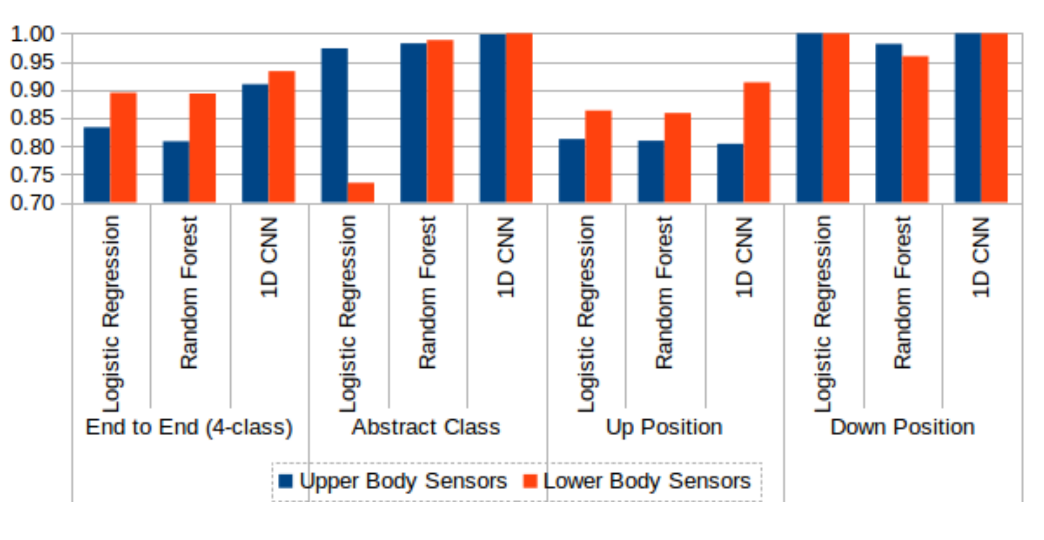
Figure 15.
Comparison of upper body (blue) and lower body (red) sensor data performance without test data sharpening. Three machine learning techniques, logistic regression, random forest, and 1D CNN, are compared on 4-class and various 2-class problems.
Figure 15.
Comparison of upper body (blue) and lower body (red) sensor data performance without test data sharpening. Three machine learning techniques, logistic regression, random forest, and 1D CNN, are compared on 4-class and various 2-class problems.
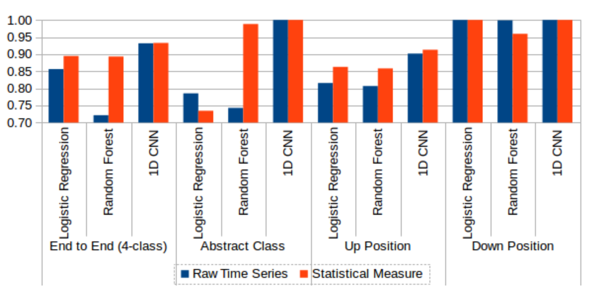
Figure 16.
Comparison of raw time series (blue) and statistical feature (red) data performance without test data sharpening. Three machine learning classifiers, logistic regression, random forest, and 1D CNN, are compared on 4-class and various 2-class problems.
Figure 16.
Comparison of raw time series (blue) and statistical feature (red) data performance without test data sharpening. Three machine learning classifiers, logistic regression, random forest, and 1D CNN, are compared on 4-class and various 2-class problems.
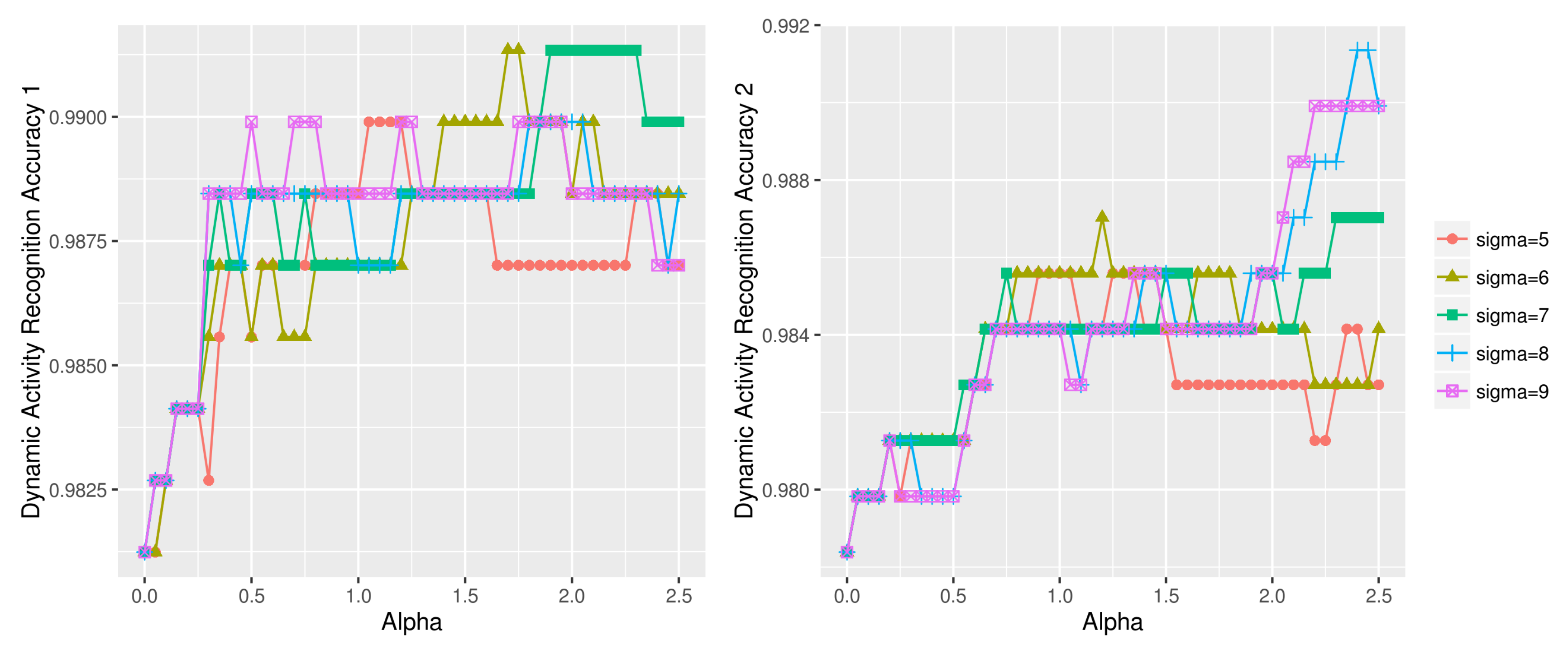
Figure 17.
Dynamic activity recognition accuracy using various (, ) combinations on UCI HAR dataset (left: dynamic test data1, right: dynamic test data2).
Figure 17.
Dynamic activity recognition accuracy using various (, ) combinations on UCI HAR dataset (left: dynamic test data1, right: dynamic test data2).
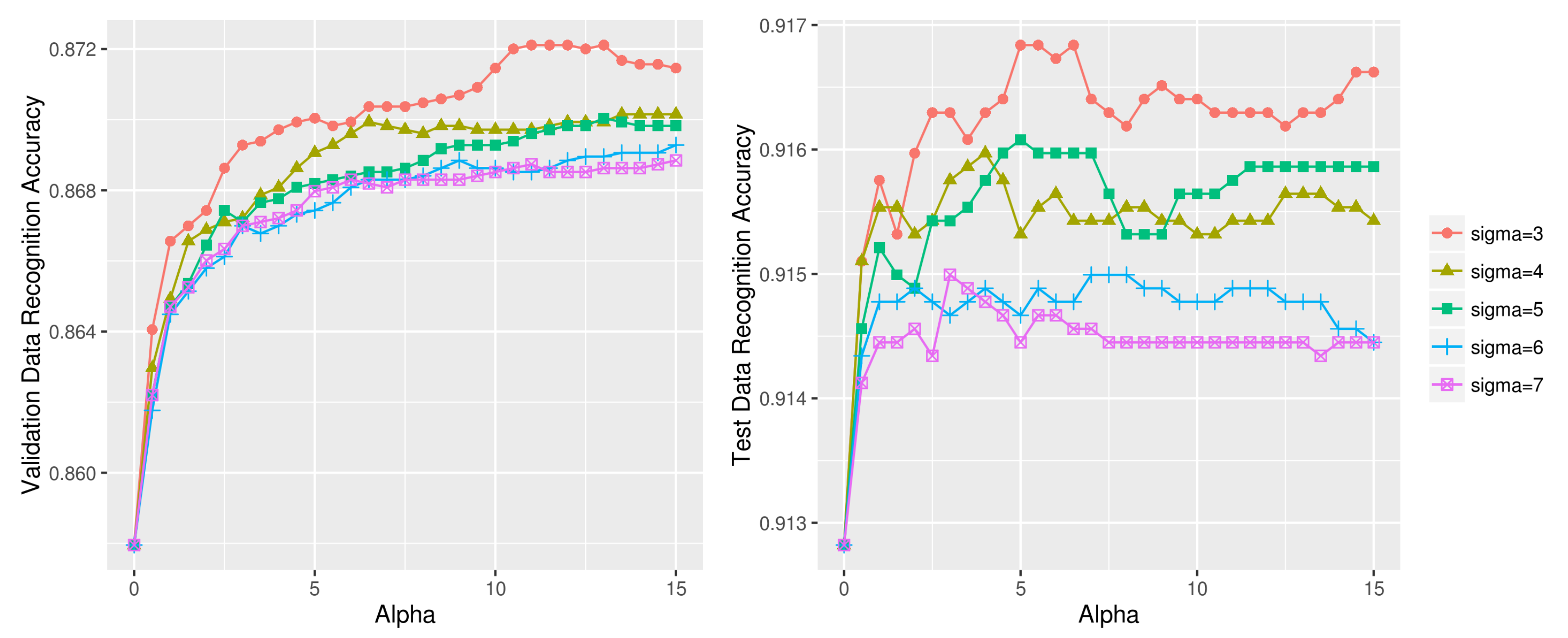
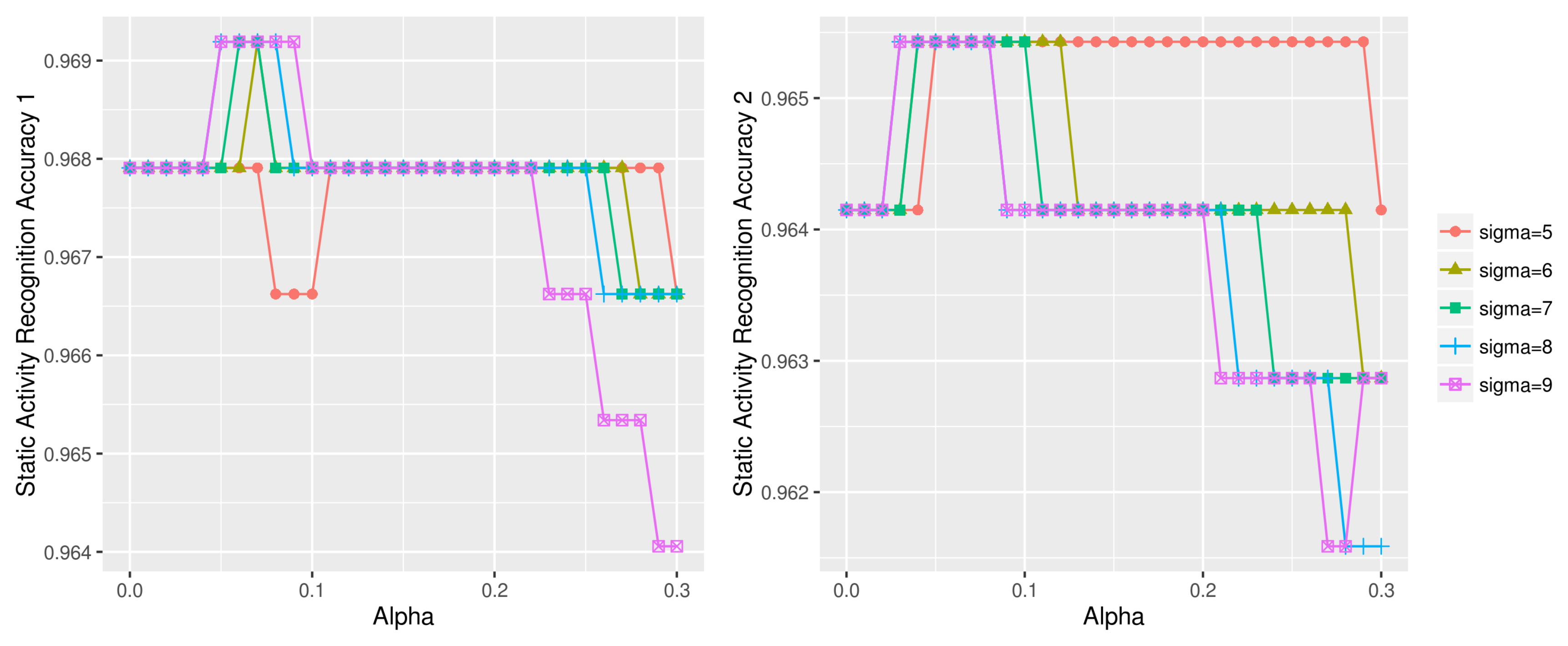
Figure 18.
Static activity recognition accuracy using various (, ) combinations on UCI HAR dataset (left: static test data1, right: static test data2).
Figure 18.
Static activity recognition accuracy using various (, ) combinations on UCI HAR dataset (left: static test data1, right: static test data2).
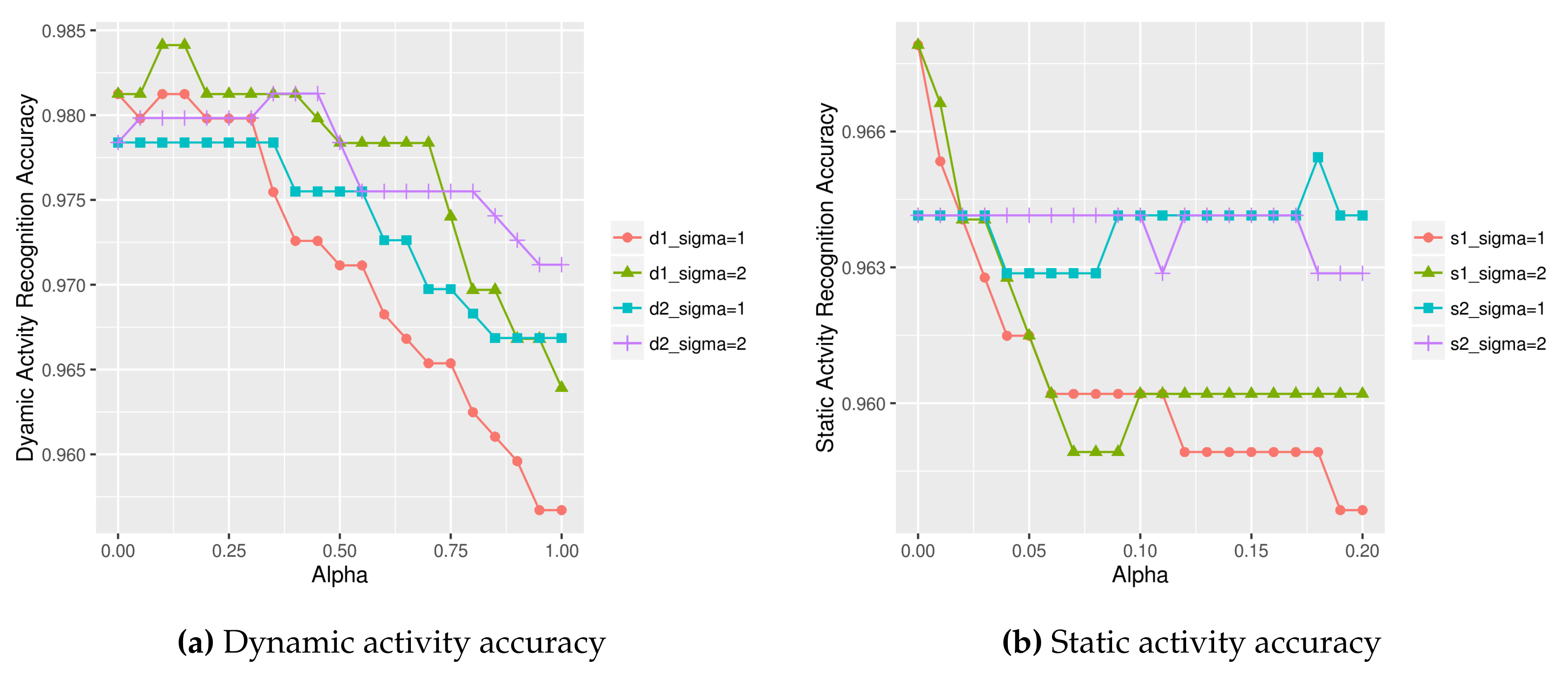
Figure 19.
Dynamic (a) and static (b) activity recognition result using on UCI HAR dataset.
Figure 19.
Dynamic (a) and static (b) activity recognition result using on UCI HAR dataset.
Table 1.
Activity class constitution and number of samples in OPPORTUNITY dataset; the same class label constitution applied to both the lower and upper body sensor data.
Table 1.
Activity class constitution and number of samples in OPPORTUNITY dataset; the same class label constitution applied to both the lower and upper body sensor data.
| Class Division | Up | Down | Total |
|---|
| Stand | Walk | Sit | Lie |
|---|
| Train | 13,250 | 7403 | 6874 | 1411 | 28,938 |
| Validate | 5964 | 3216 | 3766 | 663 | 13,609 |
| Test | 5326 | 3885 | 3460 | 793 | 13,464 |
Table 2.
Activity class constitution and number of samples in UCI HAR dataset.
Table 2.
Activity class constitution and number of samples in UCI HAR dataset.
| Class Division | Dynamic | Static | Total |
|---|
| Walking | WU* | WD* | Sitting | Standing | Laying |
|---|
| Train | 1226 | 1073 | 986 | 1286 | 1374 | 1407 | 7352 |
| Test | 496 | 471 | 420 | 491 | 532 | 537 | 2947 |
Table 3.
Test data sharpening parameter values used in evaluation experiments.
Table 3.
Test data sharpening parameter values used in evaluation experiments.
| Dataset | OPPORTUNITY | UCI HAR |
|---|
| Model | Up (lower body) | Up (upper body) | Dynamic1 | Dynamic2 | Static1 | Static2 |
|---|
| 3 | 3 | 8 | 7 | 5 | 8 |
| 13 | 12 | 2.40 | 1.95 | 0.06 | 0.07 |
Table 4.
score comparison with state of the art approach on lower body OPPORTUNITY dataset. The number in bold indicates the highest score.
Table 4.
score comparison with state of the art approach on lower body OPPORTUNITY dataset. The number in bold indicates the highest score.
| Dataset | Ordóñez and Roggen [28] (%) | Ours (%) |
|---|
| Baseline CNN | DeepConvLSTM | CNN+Sharpen |
|---|
| OPPORTUNITY | 91.2 | 93.0 | 94.2 |
Table 5.
Confusion matrix of our CNN+Sharpen approach using lower body OPPORTUNITY dataset. The bold numbers in diagonal indicate correctly classified instances; the bottom right bold number indicates the overall accuracy.
Table 5.
Confusion matrix of our CNN+Sharpen approach using lower body OPPORTUNITY dataset. The bold numbers in diagonal indicate correctly classified instances; the bottom right bold number indicates the overall accuracy.
| | Predicted Class | Recall (%) |
|---|
| Stand | Walk | Sit | Lie |
|---|
| Actual Class | Stand | 5,210 | 116 | 0 | 0 | 97.82 |
| Walk | 655 | 3,230 | 0 | 0 | 83.14 |
| Sit | 0 | 0 | 3,460 | 0 | 100.00 |
| Lie | 0 | 0 | 0 | 793 | 100.00 |
| Precision (%) | 88.83 | 96.53 | 100.00 | 100.00 | 94.27 |
Table 6.
Comparison with the state of the art approaches using UCI HAR dataset. The number in bold indicates the highest accuracy.
Table 6.
Comparison with the state of the art approaches using UCI HAR dataset. The number in bold indicates the highest accuracy.
| Approaches | Accuracy (%) |
|---|
| SVM [10] | 96.37 |
| DCNN+ [12] | 97.59 |
| FFT+Convnet [14] | 95.75 |
| TSCHMM [13] | 96.74 |
| CNN+Sharpen (Ours) | 97.62 |
Table 7.
Confusion matrix of our CNN+Sharpen approach on UCI HAR dataset. The bold numbers in diagonal indicate correctly classified instances; the bottom right bold number indicates the overall accuracy.
Table 7.
Confusion matrix of our CNN+Sharpen approach on UCI HAR dataset. The bold numbers in diagonal indicate correctly classified instances; the bottom right bold number indicates the overall accuracy.
| | Predicted Class | Recall (%) |
|---|
| Walk | WU | WD | Sit | Stand | Lay |
|---|
| Actual Class | Walk | 491 | 2 | 3 | 0 | 0 | 0 | 98.99 |
| WU | 3 | 464 | 4 | 0 | 0 | 0 | 98.51 |
| WD | 1 | 5 | 414 | 0 | 0 | 0 | 98.57 |
| Sit | 0 | 0 | 0 | 454 | 37 | 0 | 92.46 |
| Stand | 0 | 0 | 0 | 14 | 518 | 0 | 97.37 |
| Lay | 0 | 0 | 0 | 1 | 0 | 536 | 99.81 |
| Precision (%) | 99.19 | 98.51 | 98.34 | 96.80 | 93.33 | 100.00 | 97.62 |
Table 8.
Comparison of activity recognition accuracy without (1D CNN only) and with test data sharpening (1D CNN+Sharpen). The bold numbers indicate the highest accuracy for each model.
Table 8.
Comparison of activity recognition accuracy without (1D CNN only) and with test data sharpening (1D CNN+Sharpen). The bold numbers indicate the highest accuracy for each model.
| Dataset (Model) | Class | 1D CNN Only (%) | 1D CNN + Sharpen (%) |
|---|
| OPPORTUNITY (Up) | 2 | 91.28 | 91.63 |
| UCI HAR (Dynamic) | 3 | 97.98 | 98.70 |
| UCI HAR (Static) | 3 | 96.60 | 96.67 |


