Multi-Fault Diagnosis of Rolling Bearings via Adaptive Projection Intrinsically Transformed Multivariate Empirical Mode Decomposition and High Order Singular Value Decomposition


Abstract
:1. Introduction
2. Methodology
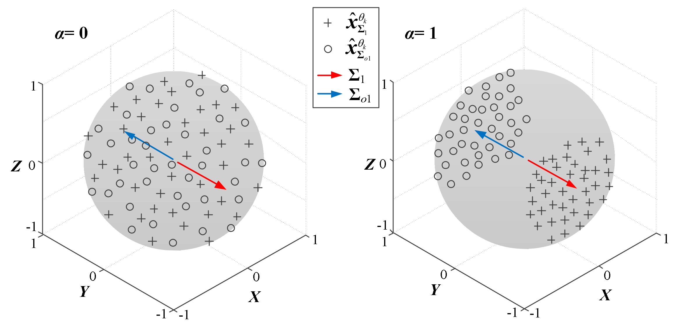
2.1. Adaptive-Projection Intrinsically Transformed Multivariate Empirical Mode Decomposition
- APIT-MEMD can align IMFs from multiple channels to the same frequency ranges, just like MEMD, and the same characteristic frequencies locate in the same orders respectively.
- APIT-MEMD can generate large numbers of adaptive projection vectors to alleviate the adverse effect of power imbalances between channels, among multi-sensor signal acquisition systems.
- APIT-MEMD has a filter bank property in the presence of Gaussian white noise; the extra noise channels can serve as references to enable more accurate and stable IMFs, in order to alleviate mode mixing problem.
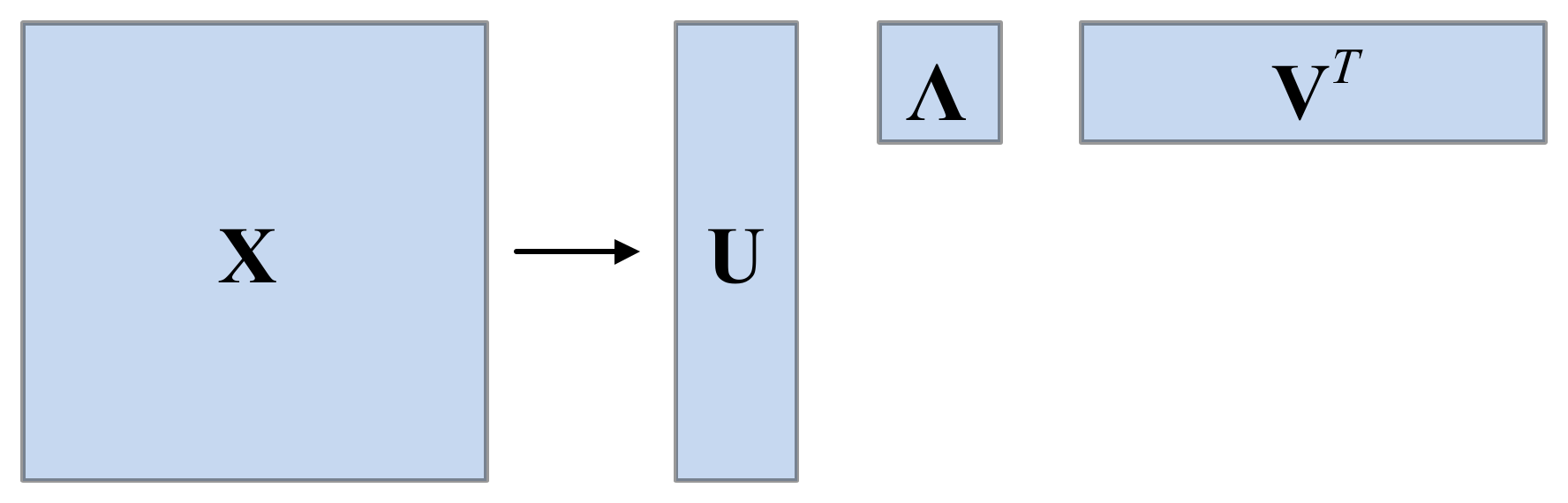
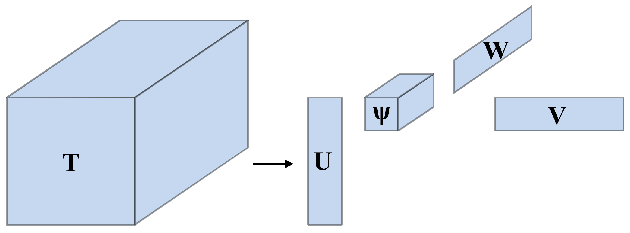
2.2. High Order Singular Value Decomposition
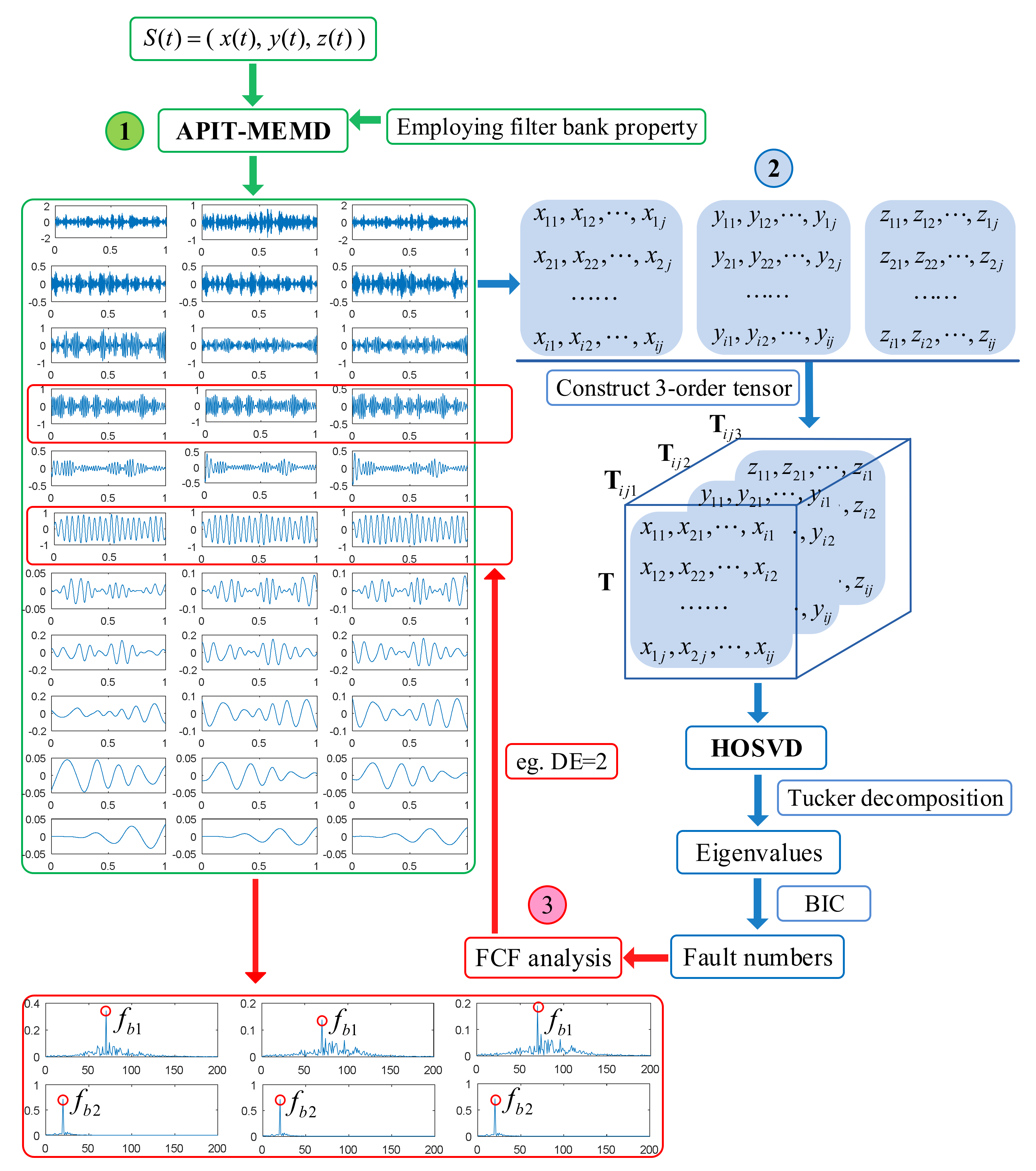
2.3. The Proposed Novel Multi-Fault Diagnosis Approach via APIT-MEMD and HOSVD
3. Numerical Simulations
3.1. Numerical Simulation of EEMD
3.2. Numerical Simulation of APIT-MEMD
3.3. Numerical Simulation of HOSVD
4. Application Researches
5. Conclusions
Acknowledgments
Author Contributions
Conflicts of Interest
References
- Lei, Y.; Lin, J.; He, Z.; Zuo, M.J. A review on empirical mode decomposition in fault diagnosis of rotating machinery. Mech. Syst. Signal Process. 2013, 35, 108–126. [Google Scholar] [CrossRef]
- Lee, D.H.; Ahn, J.H.; Koh, B.H. Fault detection of bearing systems through EEMD and optimization algorithm. Sensors 2017, 17, 2477. [Google Scholar] [CrossRef] [PubMed]
- Zhao, L.Y.; Wang, L.; Yan, R.Q. Rolling bearing fault diagnosis based on wavelet packet decomposition and multi-scale permutation entropy. Entropy 2015, 17, 6447–6461. [Google Scholar] [CrossRef]
- Li, F.; Shi, P.; Lim, C.C.; Wu, L. Fault detection filtering for nonhomogeneous markovian jump systems via fuzzy approach. IEEE Trans. Fuzzy Syst. 2016, 99, 1–12. [Google Scholar] [CrossRef]
- Chibani, A.; Chadli, M.; Ding, S.X.; Braiek, N.B. Design of robust fuzzy fault detection filter for polynomial fuzzy systems with new finite frequency specifications. Automatica 2018, 93, 42–54. [Google Scholar] [CrossRef]
- Zhao, X.; Patel, T.H.; Zuo, M.J. Multivariate EMD and full spectrum based condition monitoring for rotating machinery. Mech. Syst. Signal Process. 2012, 27, 712–728. [Google Scholar] [CrossRef]
- Li, K.; Su, L.; Wu, J.; Wang, H.; Chen, P. A rolling bearing fault diagnosis method based on variational mode decomposition and an improved kernel extreme learning machine. Appl. Sci. 2017, 7, 1004. [Google Scholar] [CrossRef]
- Tang, G.; Luo, G.; Zhang, W.; Yang, C.; Wang, H. Underdetermined blind source separation with variational mode decomposition for compound roller bearing fault signals. Sensors 2016, 16, 897. [Google Scholar] [CrossRef] [PubMed]
- Zhang, X.; Zhou, J. Multi-fault diagnosis for rolling element bearings based on ensemble empirical mode decomposition and optimized support vector machines. Mech. Syst. Signal Process. 2013, 41, 127–140. [Google Scholar] [CrossRef]
- Huang, N.E.; Shen, Z.; Long, S.R.; Wu, M.C.; Shih, H.H.; Zheng, Q.; Yen, N.C.; Tung, C.C.; Liu, H.H. The empirical mode decomposition and the Hilbert spectrum for nonlinear and non-stationary time series analysis. Proc. R. Soc. Lond. A 1998, 454, 903–995. [Google Scholar]
- Griffin, D.; Lim, J. Signal estimation from modified short-time Fourier transform. IEEE Trans. Acoust. Speech Signal Process. 1984, 32, 236–243. [Google Scholar] [CrossRef]
- Daubechies, I. The wavelet transform, time-frequency localization and signal analysis. IEEE Trans. Inf. Theory 1990, 36, 961–1005. [Google Scholar] [CrossRef]
- Wang, Z.; Chen, J.; Dong, G.; Zhou, Y. Constrained independent component analysis and its application to machine fault diagnosis. Mech. Syst. Signal Process. 2011, 25, 2501–2512. [Google Scholar] [CrossRef]
- Wu, Z.; Huang, N.E. Ensemble empirical mode decomposition: A noise-assisted data analysis method. Adv. Adapt. Data Anal. 2009, 1, 1–41. [Google Scholar] [CrossRef]
- Yi, C.; Lin, J.; Zhang, W.; Ding, J. Faults diagnostics of railway axle bearings based on IMF’s confidence index algorithm for ensemble EMD. Sensors 2015, 15, 10991–11011. [Google Scholar] [CrossRef] [PubMed]
- Wu, F.; Qu, L. An improved method for restraining the end effect in empirical mode decomposition and its applications to the fault diagnosis of large rotating machinery. J. Sound Vib. 2008, 314, 586–602. [Google Scholar] [CrossRef]
- Yeh, J.R.; Shieh, J.S.; Huang, N.E. Complementary ensemble empirical mode decomposition: A novel noise enhanced data analysis method. Adv. Adapt. Data Anal. 2010, 2, 135–156. [Google Scholar] [CrossRef]
- Looney, D.; Mandic, D.P. Multiscale image fusion using complex extensions of EMD. IEEE Trans. Signal Process. 2009, 57, 1626–1630. [Google Scholar] [CrossRef]
- Rilling, G.; Flandrin, P.; Gonçalves, P.; Lilly, J.M. Bivariate empirical mode decomposition. IEEE Signal Process. Lett. 2007, 14, 936–939. [Google Scholar] [CrossRef]
- Yang, W.; Court, R.; Tavner, P.J.; Crabtree, C.J. Bivariate empirical mode decomposition and its contribution to wind turbine condition monitoring. J. Sound Vib. 2011, 330, 3766–3782. [Google Scholar] [CrossRef]
- Ur Rehman, N.; Mandic, D.P. Empirical mode decomposition for trivariate signals. IEEE Trans. Signal Process. 2010, 58, 1059–1068. [Google Scholar] [CrossRef]
- Rehman, N.; Mandic, D.P. Multivariate empirical mode decomposition. Proc. R. Soc. A 2010, 466, 1291–1302. [Google Scholar] [CrossRef]
- Fleureau, J.; Kachenoura, A.; Albera, L.; Nunes, J.C.; Senhadji, L. Multivariate empirical mode decomposition and application to multichannel filtering. Signal Process. 2011, 91, 2783–2792. [Google Scholar] [CrossRef] [Green Version]
- Zhao, M.; Lin, J.; Xu, X.; Li, X. Multi-fault detection of rolling element bearings under harsh working condition using imf-based adaptive envelope order analysis. Sensors 2014, 14, 20320–20346. [Google Scholar] [CrossRef] [PubMed]
- Kim, J.; Lee, S.K.; Lee, B. EEG classification in a single-trial basis for vowel speech perception using multivariate empirical mode decomposition. J. Neural Eng. 2014, 11, 036010. [Google Scholar] [CrossRef] [PubMed]
- Sharma, J.B.; Sharma, K.K.; Sahula, V. Hybrid image fusion scheme using self-fractional Fourier functions and multivariate empirical mode decomposition. Signal Process. 2014, 100, 146–159. [Google Scholar] [CrossRef]
- Lv, Y.; Yuan, R.; Song, G. Multivariate empirical mode decomposition and its application to fault diagnosis of rolling bearing. Mech. Syst. Signal Process. 2016, 81, 219–234. [Google Scholar] [CrossRef]
- Hemakom, A.; Goverdovsky, V.; Looney, D.; Mandic, D.P. Adaptive-projection intrinsically transformed multivariate empirical mode decomposition in cooperative brain–computer interface applications. Phil. Trans. R. Soc. A 2016, 374, 20150199. [Google Scholar] [CrossRef] [PubMed]
- Flandrin, P.; Rilling, G.; Goncalves, P. Empirical mode decomposition as a filter bank. IEEE Signal Process. Lett. 2004, 11, 112–114. [Google Scholar] [CrossRef]
- Ur Rehman, N.; Mandic, D.P. Filter bank property of multivariate empirical mode decomposition. IEEE Trans. Signal Process. 2011, 59, 2421–2426. [Google Scholar] [CrossRef]
- Klema, V.; Laub, A. The singular value decomposition: Its computation and some applications. IEEE Trans. Autom. Control 1980, 25, 164–176. [Google Scholar] [CrossRef]
- Deshun, S.Y.Y.S.K. New Method of Blind Source Separation in Under-determined Mixtures Based on Singular Value Decomposition and Application. J. Mech. Eng. 2009, 8, 013. [Google Scholar]
- Dong, S.; Tang, B.; Zhang, Y. A repeated single-channel mechanical signal blind separation method based on morphological filtering and singular value decomposition. Measurement 2012, 45, 2052–2063. [Google Scholar] [CrossRef]
- Zhou, L.; Li, C. Outsourcing eigen-decomposition and singular value decomposition of large matrix to a public cloud. IEEE Access 2016, 4, 869–879. [Google Scholar] [CrossRef]
- Yi, C.; Lv, Y.; Ge, M.; Xiao, H.; Yu, X. Tensor singular spectrum decomposition algorithm based on permutation entropy for rolling bearing fault diagnosis. Entropy 2017, 19, 139. [Google Scholar] [CrossRef]
- Sun, H.; Guo, J.; Fang, L. Improved Singular Value Decomposition (TopSVD) for Source Number Estimation of Low SNR in Blind Source Separation. IEEE Access 2017, 5, 26460–26465. [Google Scholar] [CrossRef]
- Vrabie, V.D.; Le Bihan, N.; Mars, J.I. Multicomponent wave separation using HOSVD/unimodal-ICA subspace method. Geophysics 2016, 71, V133–V143. [Google Scholar] [CrossRef]
- Ergin, S.; Çakir, S.; Gerek, Ö.N.; Gülmezoğlu, M.B. A new implementation of common matrix approach using third-order tensors for face recognition. Expert Syst. Appl. 2011, 38, 3246–3251. [Google Scholar] [CrossRef]
- Cichocki, A.; Mandic, D.; De Lathauwer, L.; Zhou, G.; Zhao, Q.; Caiafa, C.; Phan, H.A. Tensor decompositions for signal processing applications: From two-way to multiway component analysis. IEEE Signal Process. Mag. 2015, 32, 145–163. [Google Scholar] [CrossRef]
- Bousse, M.; Debals, O.; De Lathauwer, L. A tensor-based method for large-scale blind source separation using segmentation. IEEE Trans. Signal Process. 2017, 65, 346–358. [Google Scholar] [CrossRef]
- Haardt, M.; Roemer, F.; Del Galdo, G. Higher-order SVD-based subspace estimation to improve the parameter estimation accuracy in multidimensional harmonic retrieval problems. IEEE Trans. Signal Process. 2008, 56, 3198–3213. [Google Scholar] [CrossRef]
- Yi, C.; Lv, Y.; Xiao, H.; You, G.; Dang, Z. Research on the Blind Source Separation Method Based on Regenerated Phase-Shifted Sinusoid-Assisted EMD and Its Application in Diagnosing Rolling-Bearing Faults. Appl. Sci. 2017, 7, 414. [Google Scholar] [CrossRef]
- Ye, H.; Yang, S.; Yang, J. Mechanical vibration source number estimation based on emd-svd-bic. J. Vib. Measur. Diagn. 2010, 30, 330–334. [Google Scholar]
- Hemakom, A.; Ahrabian, A.; Looney, D.; ur pRehman, N.; Mandic, D.P. Nonuniformly sampled trivariate empirical mode decomposition. In Proceedings of the 2015 IEEE International Conference on Acoustics, Speech and Signal Processing (ICASSP), Brisbane, QLD, Australia, 19–24 April 2015; pp. 3691–3695. [Google Scholar]
- Lee, S.K.; White, P.R. The enhancement of impulsive noise and vibration signals for fault detection in rotating and reciprocating machinery. J. Sound Vib. 1998, 217, 485–505. [Google Scholar] [CrossRef]
- Xunjia, W.W.C.X.S. Blind Source Separation of Single-channel Mechanical Signal Based on Empirical Mode Decomposition. J. Mech. Eng. 2011, 4, 004. [Google Scholar]
- Lv, Y.; Zhu, Q.; Yuan, R. Fault diagnosis of rolling bearing based on fast nonlocal means and envelop spectrum. Sensors 2015, 15, 1182–1198. [Google Scholar] [CrossRef] [PubMed]


|
|
| Fault Type | Fault Frequency (/Hz) |
|---|---|
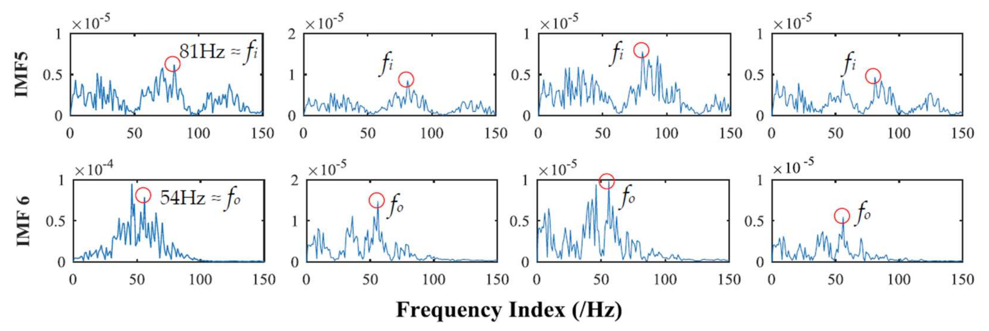
| Inner ring fault | fi = 81.45 |
| Outer ring fault | fo = 53.58 |
| 1 | 2 | 3 | 4 | 5 | |
| 0.1032 | 0.0974 | 0.1033 | 0.3525 | 0.32007 | |
| 6 | 7 | 8 | 9 | 10 | |
| 0.1210 | 0.0583 | 0.0652 | 0.0296 | 0.0067 |
© 2018 by the authors. Licensee MDPI, Basel, Switzerland. This article is an open access article distributed under the terms and conditions of the Creative Commons Attribution (CC BY) license (http://creativecommons.org/licenses/by/4.0/).
Share and Cite
Yuan, R.; Lv, Y.; Song, G. Multi-Fault Diagnosis of Rolling Bearings via Adaptive Projection Intrinsically Transformed Multivariate Empirical Mode Decomposition and High Order Singular Value Decomposition. Sensors 2018, 18, 1210. https://doi.org/10.3390/s18041210
Yuan R, Lv Y, Song G. Multi-Fault Diagnosis of Rolling Bearings via Adaptive Projection Intrinsically Transformed Multivariate Empirical Mode Decomposition and High Order Singular Value Decomposition. Sensors. 2018; 18(4):1210. https://doi.org/10.3390/s18041210
Chicago/Turabian StyleYuan, Rui, Yong Lv, and Gangbing Song. 2018. "Multi-Fault Diagnosis of Rolling Bearings via Adaptive Projection Intrinsically Transformed Multivariate Empirical Mode Decomposition and High Order Singular Value Decomposition" Sensors 18, no. 4: 1210. https://doi.org/10.3390/s18041210
APA StyleYuan, R., Lv, Y., & Song, G. (2018). Multi-Fault Diagnosis of Rolling Bearings via Adaptive Projection Intrinsically Transformed Multivariate Empirical Mode Decomposition and High Order Singular Value Decomposition. Sensors, 18(4), 1210. https://doi.org/10.3390/s18041210