Automated Geo/Co-Registration of Multi-Temporal Very-High-Resolution Imagery


Abstract
:1. Introduction
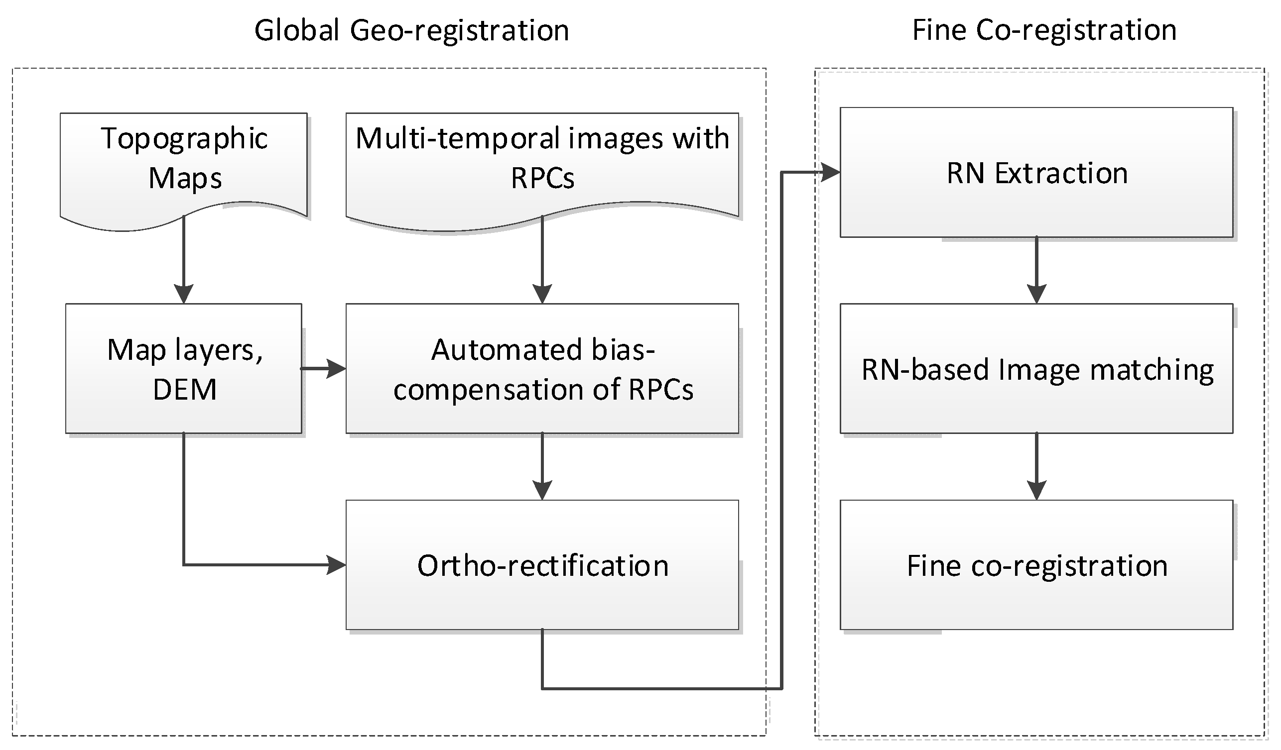
2. Methods
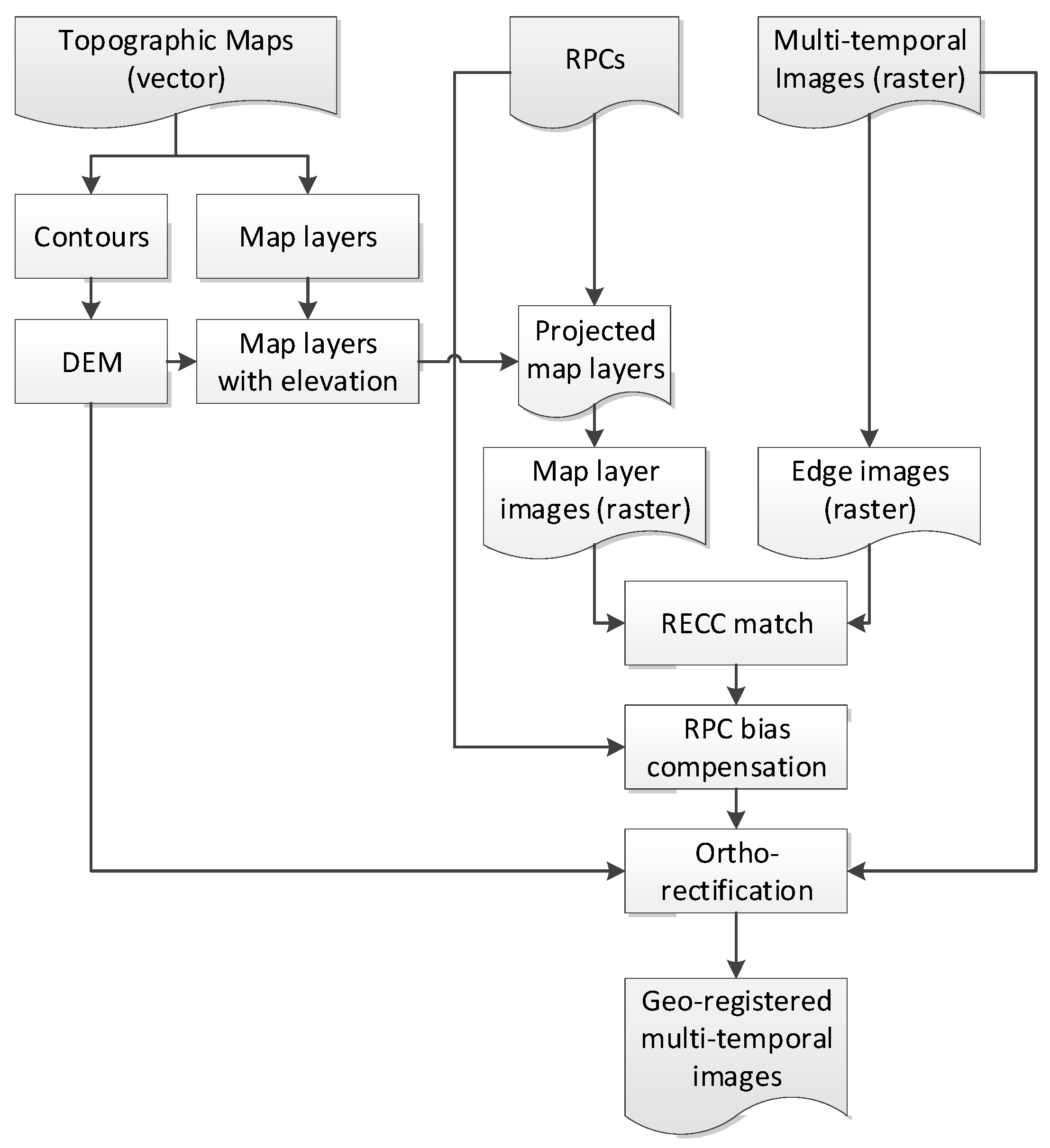
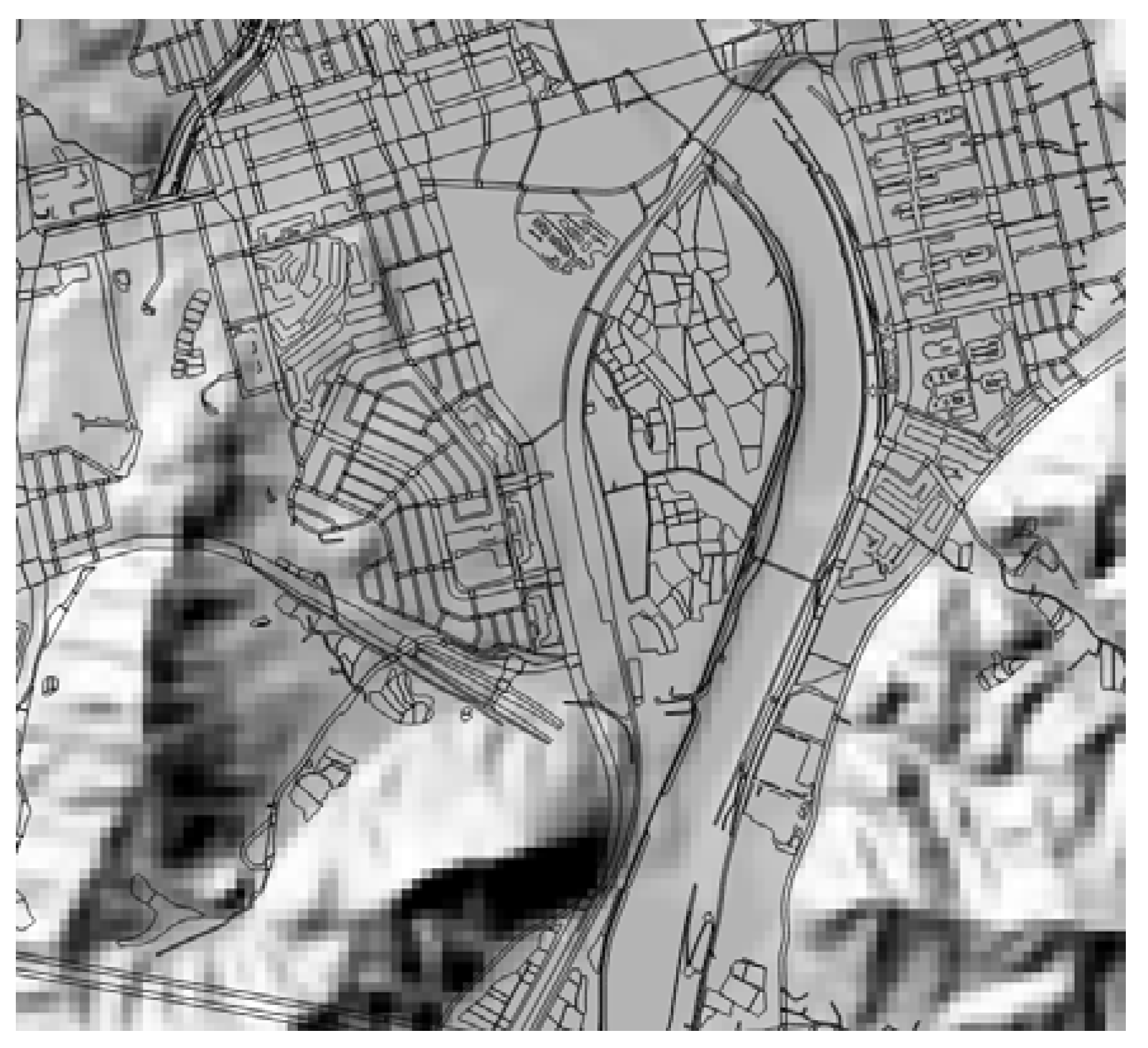
2.1. Global Georegistration
2.2. RN-Based Fine Co-Registration
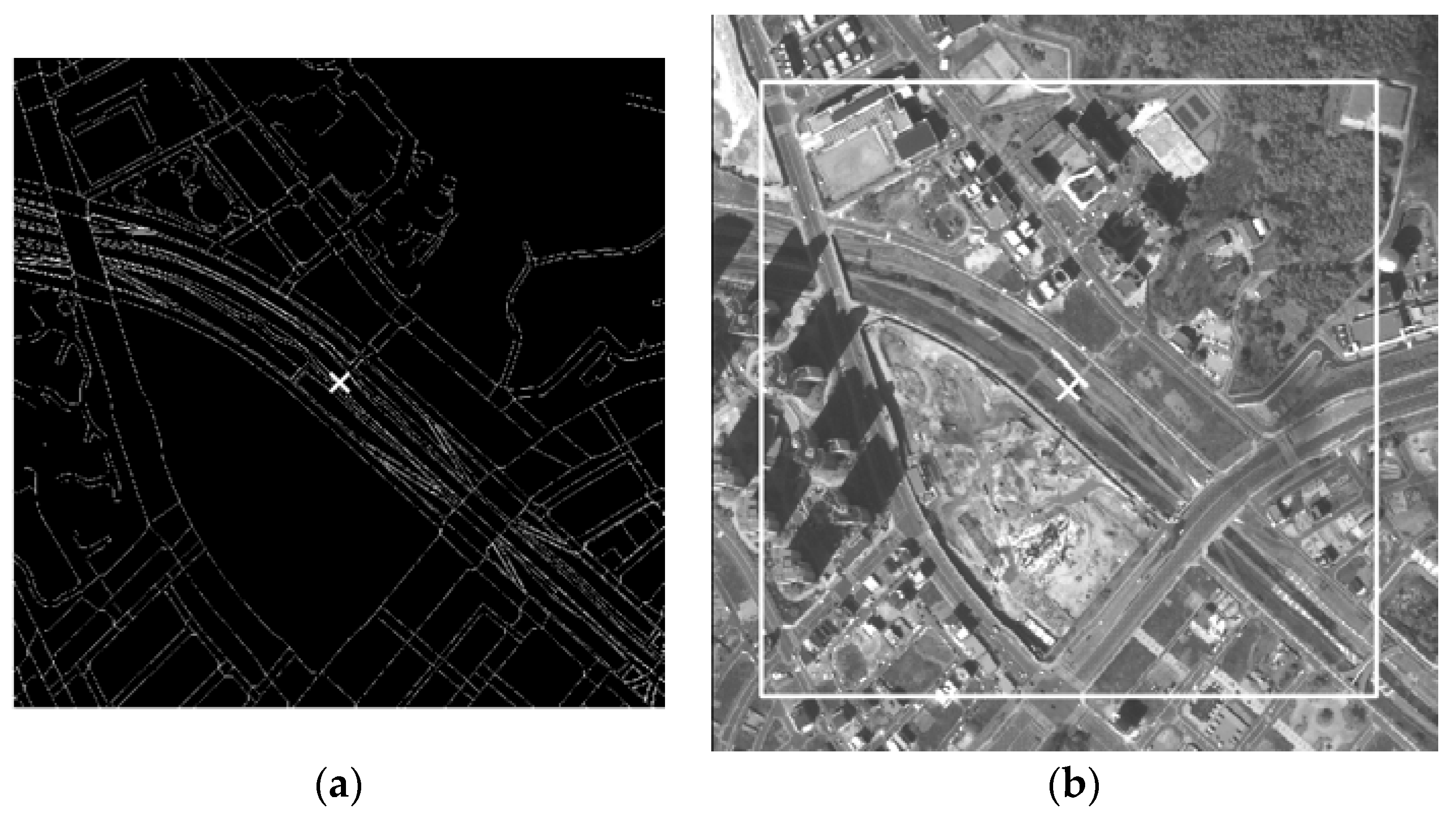
2.2.1. RN Extraction
2.2.2. Extraction of CPs for the Reference Image
2.2.3. RN-Based Image Matching
3. Experiments and Results
3.1. Dataset Construction
3.2. Global Georegistration Results
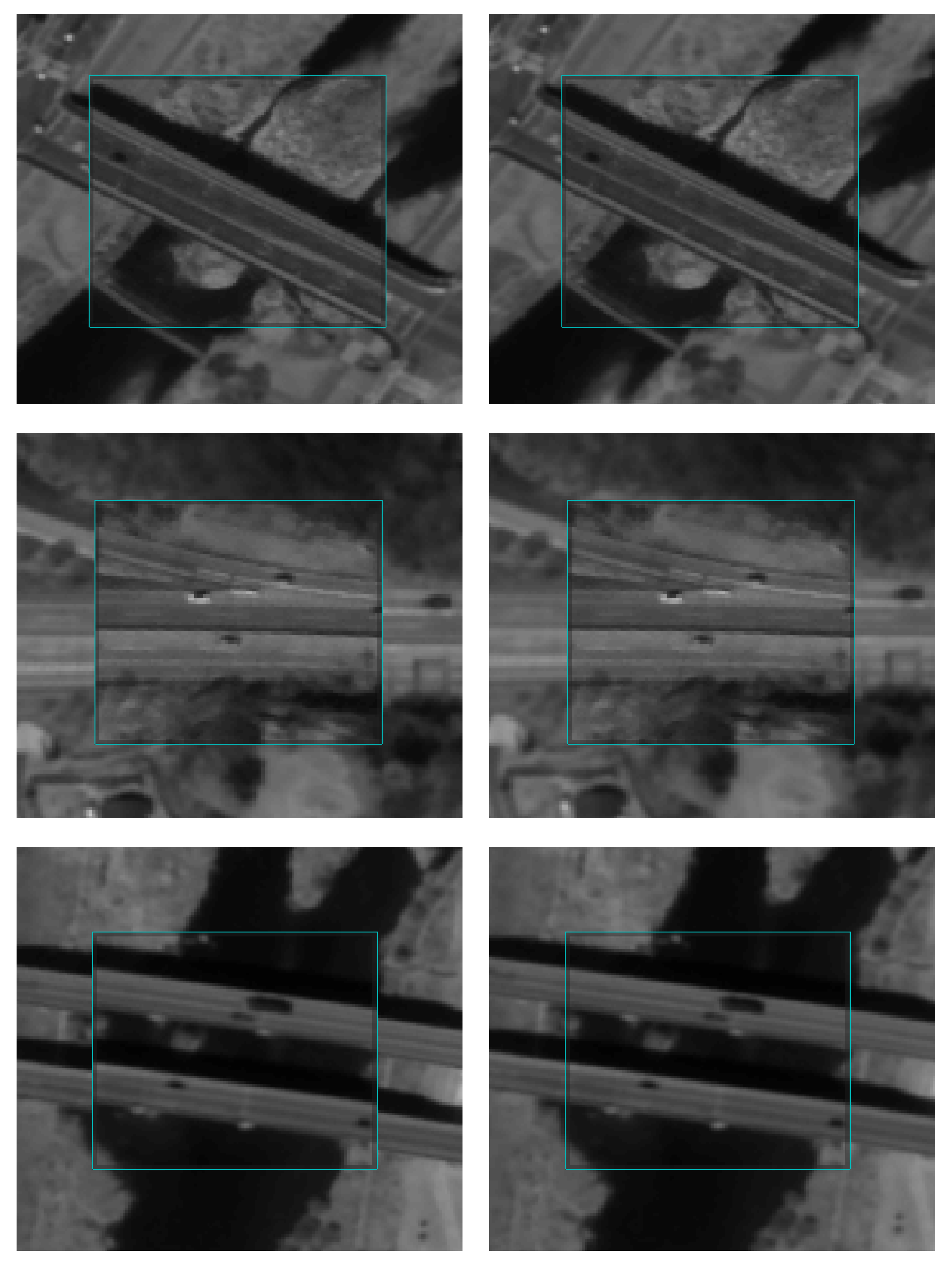
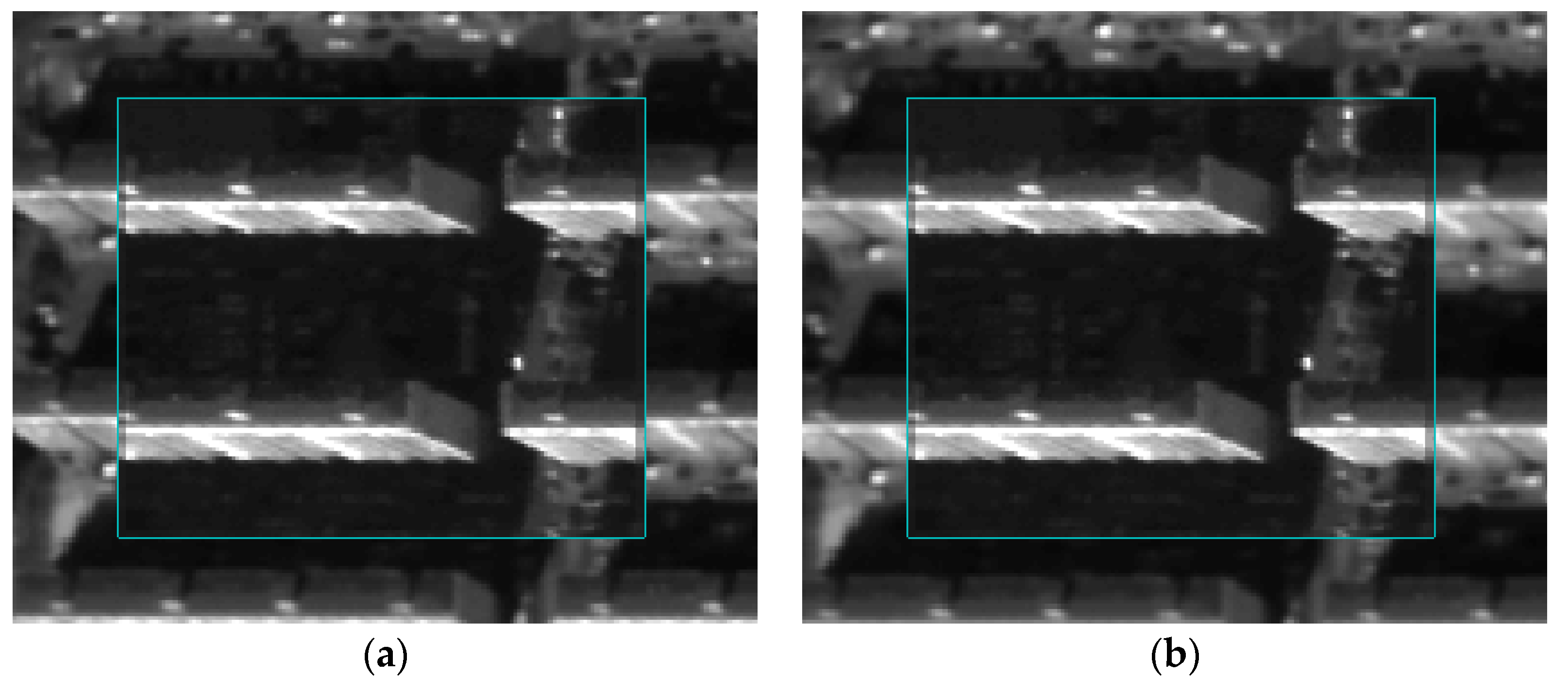
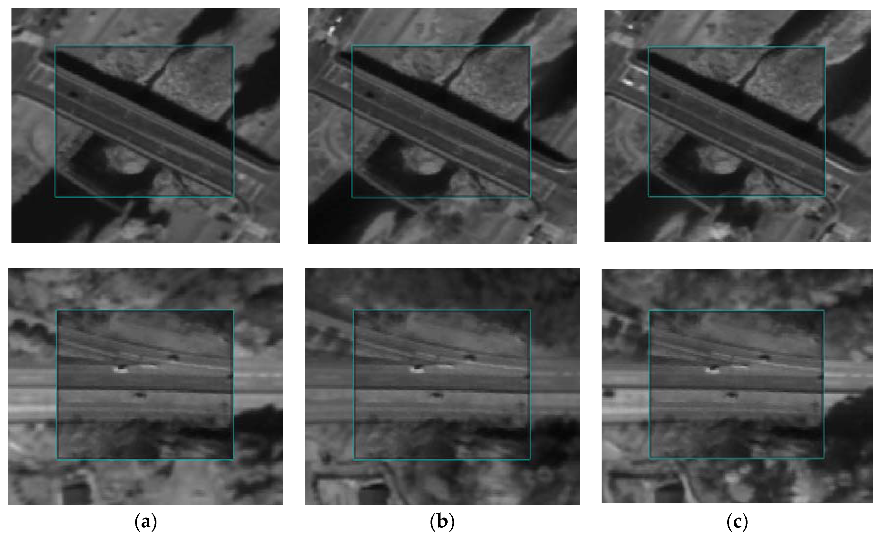
3.3. Fine Co-Registration Results
4. Conclusions
Author Contributions
Acknowledgments
Conflicts of Interest
References
- Zhao, Y. Crop growth dynamics modeling using time-series satellite imagery. Land Surf. Remote Sens. II 2014, 9260, 926003. [Google Scholar] [CrossRef]
- Mennis, J.; Viger, R. Analyzing time series of satellite imagery using temporal map algebra. In Proceedings of the ASPRS 2004 Annual Convention, Denver, CO, USA, 23–28 May 2004; pp. 23–28. [Google Scholar]
- Laneve, G.; Cadau, E.G.; De Rosa, D. Change detection analysis on time series of satellite images with variable illumination conditions and spatial resolution. In Proceedings of the MultiTemp 2007. International Workshop on the Analysis of Multi-temporal Remote Sensing Images, Leuven, Belgium, 18–20 July 2007. [Google Scholar]
- Yang, X.; Lo, C.P. Using a time series of satellite imagery to detect land use and land cover changes in the Atlanta, Georgia metropolitan area. Int. J. Remote Sens. 2002, 23, 1775–1798. [Google Scholar] [CrossRef]
- Stumpf, A.; Malet, J.P.; Delacourt, C. Correlation of satellite image time-series for the detection and monitoring of slow-moving landslides. Remote Sens. Environ. 2017, 189, 40–55. [Google Scholar] [CrossRef]
- Behling, R.; Roessner, S.; Segl, K.; Kleinschmit, B.; Kaufmann, H. Robust automated image co-registration of optical multi-sensor time series data: Database generation for multi-temporal landslide detection. Remote Sens. 2014, 6, 2572–2600. [Google Scholar] [CrossRef]
- Aguilar, M.A.; del Mar Saldana, M.; Aguilar, F.J. Assessing geometric accuracy of the orthorectification process from GeoEye-1 and WorldView-2 panchromatic images. Int. J. Appl. Earth Obs. 2013, 21, 427–435. [Google Scholar] [CrossRef]
- Oh, J.; Lee, C. Automated bias-compensation of rational polynomial coefficients of high resolution satellite imagery based on topographic maps. ISPRS J. Photogramm. Remote Sens. 2015, 100, 14–22. [Google Scholar] [CrossRef]
- Teo, T.A. Bias compensation in a rigorous sensor model and rational function model for high-resolution satellite images. Photogramm. Eng. Remote Sens. 2011, 77, 1211–1220. [Google Scholar] [CrossRef]
- Shen, X.; Li, Q.; Wu, G.; Zhu, J. Bias compensation for rational polynomial coefficients of high-resolution satellite imagery by local polynomial modeling. Remote Sens. 2017, 9, 200. [Google Scholar] [CrossRef]
- Konugurthi, P.K.; Kune, R.; Nooka, R.; Sarma, V. Autonomous ortho-rectification of very high resolution imagery using SIFT and genetic algorithm. Photogramm. Eng. Remote Sens. 2016, 82, 377–388. [Google Scholar] [CrossRef]
- Fraser, C.S.; Hanley, H.B. Bias-compensated RPCs for sensor orientation of high-resolution satellite imagery. Photogramm. Eng. Remote Sens. 2005, 71, 909–915. [Google Scholar] [CrossRef]
- Oh, J.; Lee, C.; Seo, D.C. Automated HRSI georegistration using orthoimage and SRTM: Focusing KOMPSAT-2 imagery. Comput Geosci. 2013, 52, 77–84. [Google Scholar] [CrossRef]
- Pan, H.; Tao, C.; Zou, Z. Precise georeferencing using the rigorous sensor model and rational function model for ZiYuan-3 strip scenes with minimum control. ISPRS J. Photogramm. Remote Sens. 2016, 119, 259–266. [Google Scholar] [CrossRef]
- Zitová, B.; Flusser, J. Image registration methods: A survey. Image Vis. Comput. 2003, 21, 977–1000. [Google Scholar] [CrossRef]
- Huo, C.; Pan, C.; Huo, L.; Zhou, Z. Multilevel SIFT matching for large-size VHR image registration. IEEE Geosci. Remote Sens. Lett. 2012, 9, 171–175. [Google Scholar] [CrossRef]
- Yu, L.; Zhang, D.; Holden, E.J. A fast and fully automatic registration approach based on point features for multi-source remote-sensing images. Comput. Geosci. 2008, 34, 838–848. [Google Scholar] [CrossRef]
- Lowe, D.G. Distinctive image features from scale-invariant keypoints. Int. J. Comput. Vis. 2004, 60, 91–110. [Google Scholar] [CrossRef]
- Bay, H.; Ess, A.; Tuytelaars, T.; Van Gool, L. Speeded-up robust features (SURF). Comput. Vis. Image Underst. 2008, 110, 346–359. [Google Scholar] [CrossRef]
- Oh, J.; Lee, C.; Eo, Y.; Bethel, J. Automated georegistration of high-resolution satellite imagery using a RPC model with airborne lidar information. Photogramm. Eng. Remote Sens. 2012, 78, 1045–1056. [Google Scholar] [CrossRef]
- Han, Y.; Bovolo, F.; Bruzzone, L. An approach to fine coregistration between very high resolution multispectral images based on registration noise distribution. IEEE Trans. Geosci. Remote Sens. 2015, 53, 6650–6662. [Google Scholar] [CrossRef]
- Hong, G.; Zhang, Y. Wavelet-based image registration technique for high-resolution remote sensing images. Comput. Geosci. 2008, 34, 1708–1720. [Google Scholar] [CrossRef]
- Arévalo, V.; González, J. Improving piecewise linear registration of high-resolution satellite images through mesh optimization. IEEE Trans. Geosci. Remote Sens. 2008, 46, 3792–3803. [Google Scholar] [CrossRef]
- Han, Y.; Choi, J.; Byun, Y.; Kim, Y. Parameter optimization for the extraction of matching points between high-resolution multisensory images in urban areas. IEEE Trans. Geosci. Remote Sens. 2014, 52, 5612–5621. [Google Scholar]
- Ye, Y.; Shan, J. A local descriptor based registration method for multispectral remote sensing images with non-linear intensity differences. ISPRS J. Photogramm. Remote Sens. 2014, 90, 83–95. [Google Scholar] [CrossRef]
- Han, Y.; Bovolo, F.; Bruzzone, L. Segmentation-based fine registration of very high resolution multitemporal images. IEEE Trans. Geosci. Remote Sens. 2017, 55, 2884–2897. [Google Scholar] [CrossRef]
- Habib, A.; Han, Y.; Xiong, W.; He, F.; Zhang, Z.; Crawford, M. Automated ortho-rectification of UAV-based hyperspectral data over an agricultural field using frame RGB imagery. Remote Sens. 2016, 8, 796. [Google Scholar] [CrossRef]
- Aicardi, I.; Nex, F.; Gerke, M.; Lingua, A.M. An Image-Based Approach for the Co-Registration of Multi-Temporal UAV Image Datasets. Remote Sens. 2016, 8, 779. [Google Scholar] [CrossRef]
- Han, Y.; Bovolo, F.; Bruzzone, L. Edge-based registration-noise estimation in VHR multitemporal and multisensor images. IEEE Geosci. Remote Sens. Lett. 2016, 13, 1231–1235. [Google Scholar] [CrossRef]
- Carson, C.; Belongie, S.; Greenspan, H.; Malik, J. Blobworld: Image segmentation using expectation-maximization and its application to image querying. IEEE Trans. Pattern Anal. Mach. Intell. 2002, 24, 1026–1038. [Google Scholar] [CrossRef]


| Sensor | Kompsat-3 | ||||
|---|---|---|---|---|---|
| Scene ID | K3-1 | K3-2 | K3-3 | K3-4 | K3-5 |
| Spatial resolution | 0.7 m | 0.7 m | 0.7 m | 0.7 m | 0.7 m |
| Processing level | 1R | 1R | 1R | 1R | 1R |
| Acquisition date | 7 February 2016 | 25 March 2015 | 23 October 2014 | 3 March 2014 | 16 November 2013 |
| Incidence/azimuth | 38.0°/196.8° | 23.2°/125.4° | 25.6°/238.1° | 12.1°/146.4° | 10.1°/260.6° |
| Size (line ×sample) | 20,452 × 24,060 pixels | 21,280 × 24,060 pixels | 20,464 × 24,060 pixels | 21,740 × 24,060 pixels | 22,376 × 24,060 pixels |
| Scene ID | Number of Outliers [Points] | Bias Precision before Outlier Removal (col/row) [Pixels] | Bias Precision after Outlier Removal (col/row) [Pixels] |
|---|---|---|---|
| K3-1 | 17 | 1.89/5.01 | 0.51/0.59 |
| K3-2 | 5 | 2.50/2.81 | 1.90/1.68 |
| K3-3 | 9 | 0.90/0.86 | 0.75/0.74 |
| K3-4 | 17 | 2.86/3.27 | 1.21/0.99 |
| K3-5 | 4 | 1.16/1.93 | 0.81/0.93 |
| Reference Image | Sensed Image | Number of Corresponding Points | Correlation Coefficient (RECC) | Correlation Coefficient (RNCC) |
|---|---|---|---|---|
| K3-1 | K3-2 | 2455 | 0.757 | 0.799 |
| K3-3 | 1591 | 0.583 | 0.625 | |
| K3-4 | 3014 | 0.774 | 0.818 | |
| K3-5 | 3095 | 0.687 | 0.734 | |
| K3-2 | K3-3 | 665 | 0.539 | 0.591 |
| K3-4 | 1159 | 0.841 | 0.851 | |
| K3-5 | 617 | 0.630 | 0.663 | |
| K3-3 | K3-4 | 1831 | 0.622 | 0.664 |
| K3-5 | 1323 | 0.710 | 0.742 | |
| K3-4 | K3-5 | 1772 | 0.757 | 0.785 |
© 2018 by the authors. Licensee MDPI, Basel, Switzerland. This article is an open access article distributed under the terms and conditions of the Creative Commons Attribution (CC BY) license (http://creativecommons.org/licenses/by/4.0/).
Share and Cite
Han, Y.; Oh, J. Automated Geo/Co-Registration of Multi-Temporal Very-High-Resolution Imagery. Sensors 2018, 18, 1599. https://doi.org/10.3390/s18051599
Han Y, Oh J. Automated Geo/Co-Registration of Multi-Temporal Very-High-Resolution Imagery. Sensors. 2018; 18(5):1599. https://doi.org/10.3390/s18051599
Chicago/Turabian StyleHan, Youkyung, and Jaehong Oh. 2018. "Automated Geo/Co-Registration of Multi-Temporal Very-High-Resolution Imagery" Sensors 18, no. 5: 1599. https://doi.org/10.3390/s18051599
APA StyleHan, Y., & Oh, J. (2018). Automated Geo/Co-Registration of Multi-Temporal Very-High-Resolution Imagery. Sensors, 18(5), 1599. https://doi.org/10.3390/s18051599