Radar and Visual Odometry Integrated System Aided Navigation for UAVS in GNSS Denied Environment


Abstract
:1. Introduction
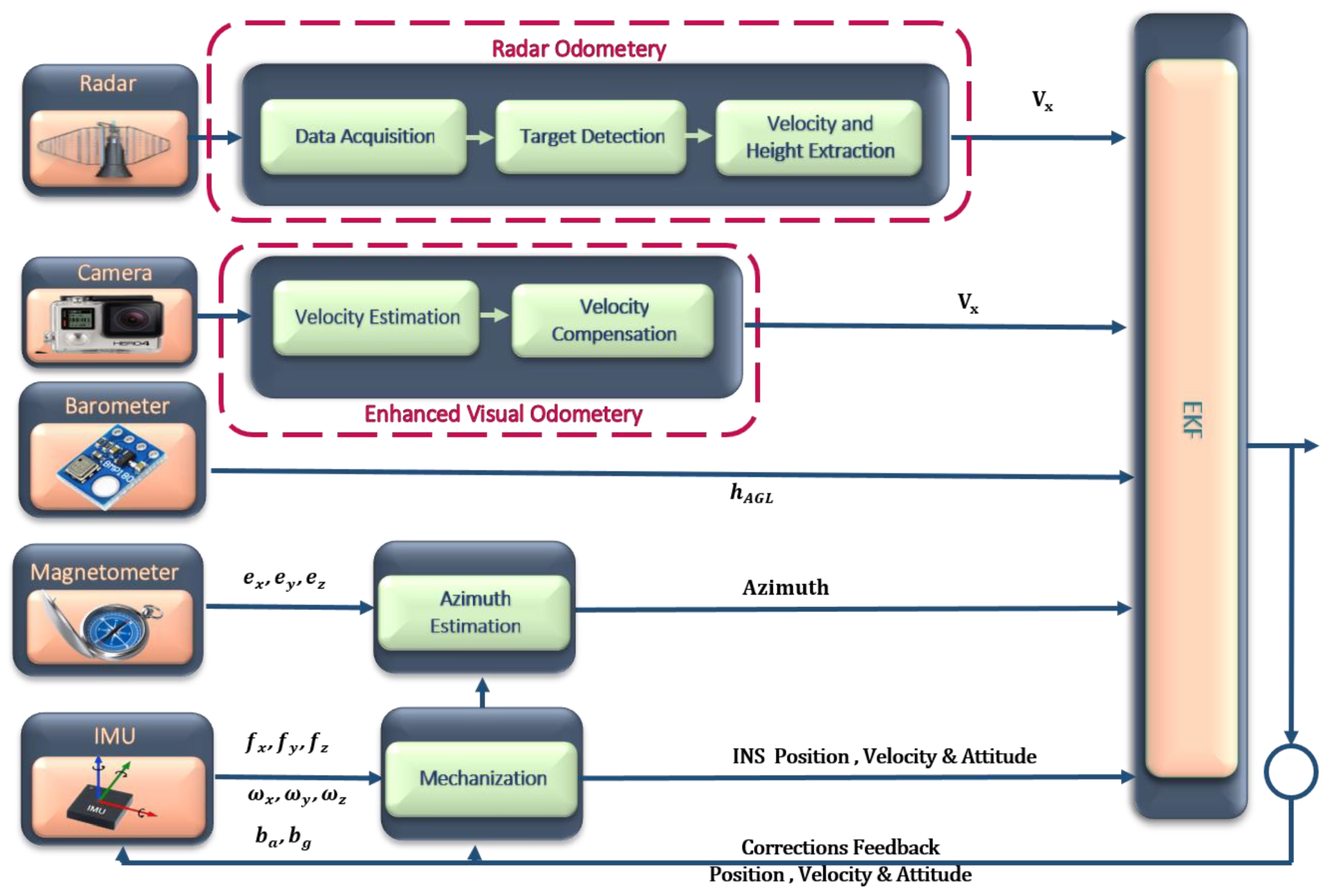
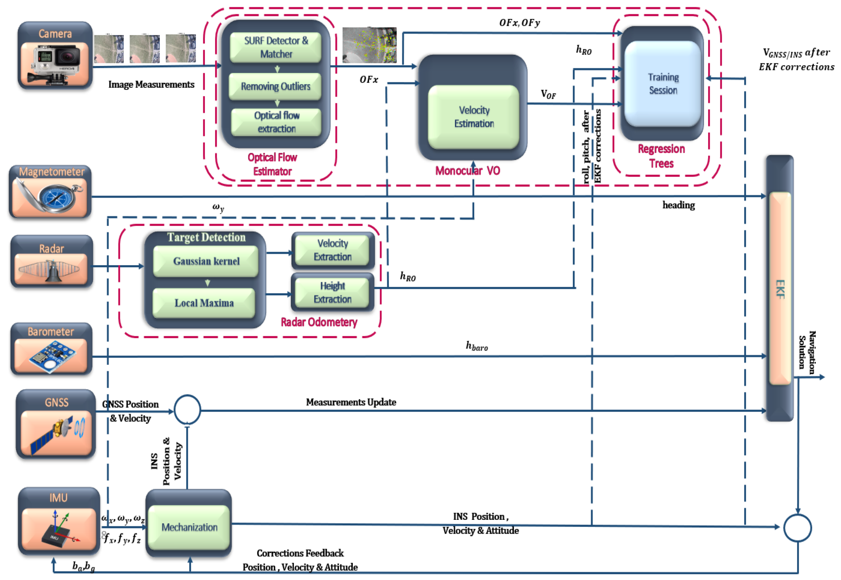
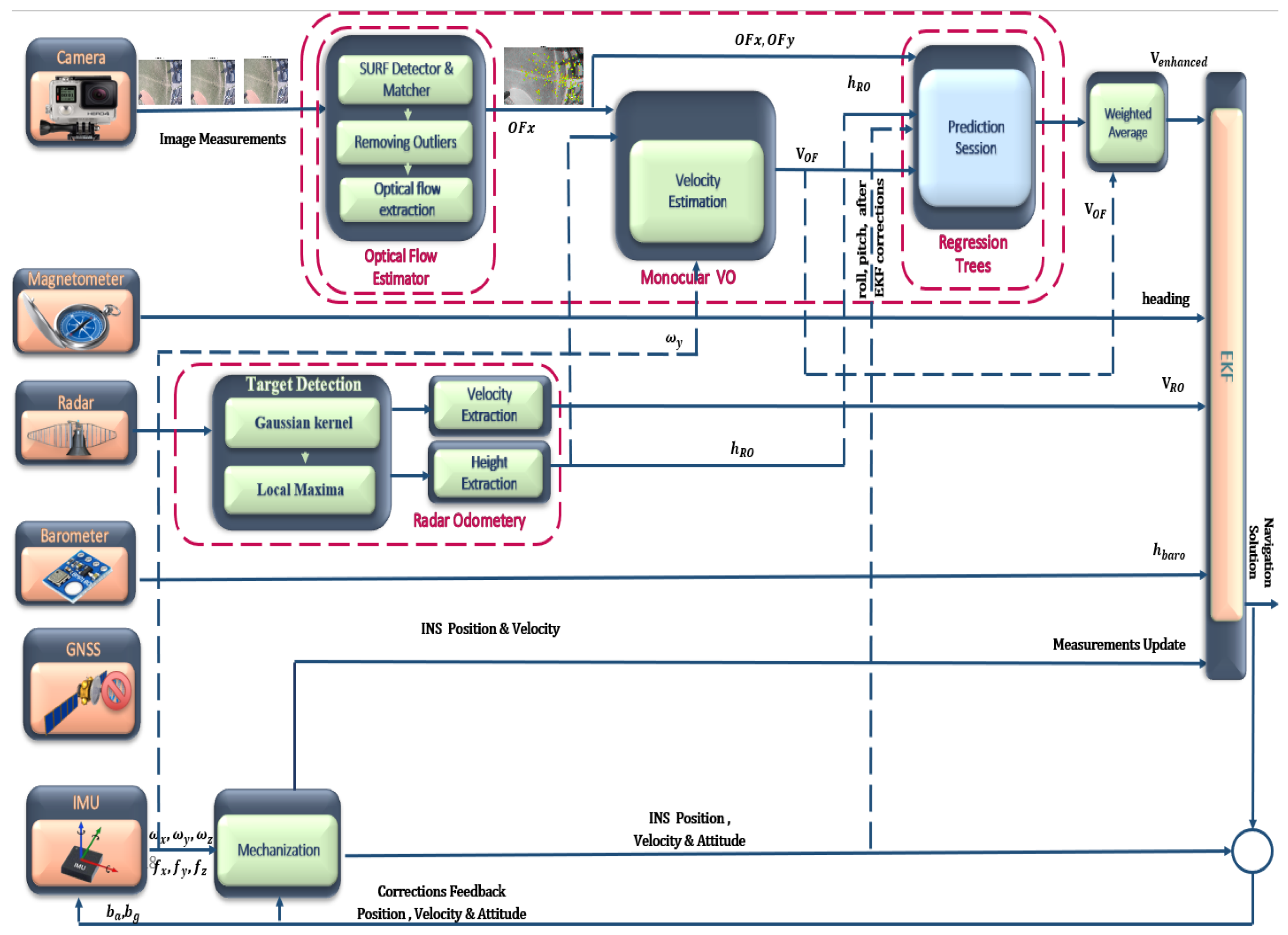
2. System Overview of the Proposed Algorithm
2.1. Frequency Modulated Continuous Wave Radar Odometry
2.1.1. Data Acquisition
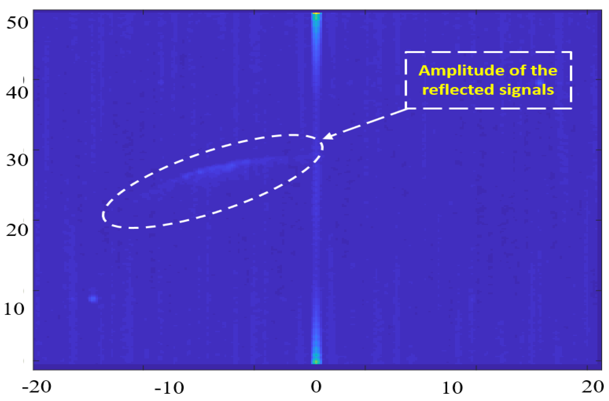
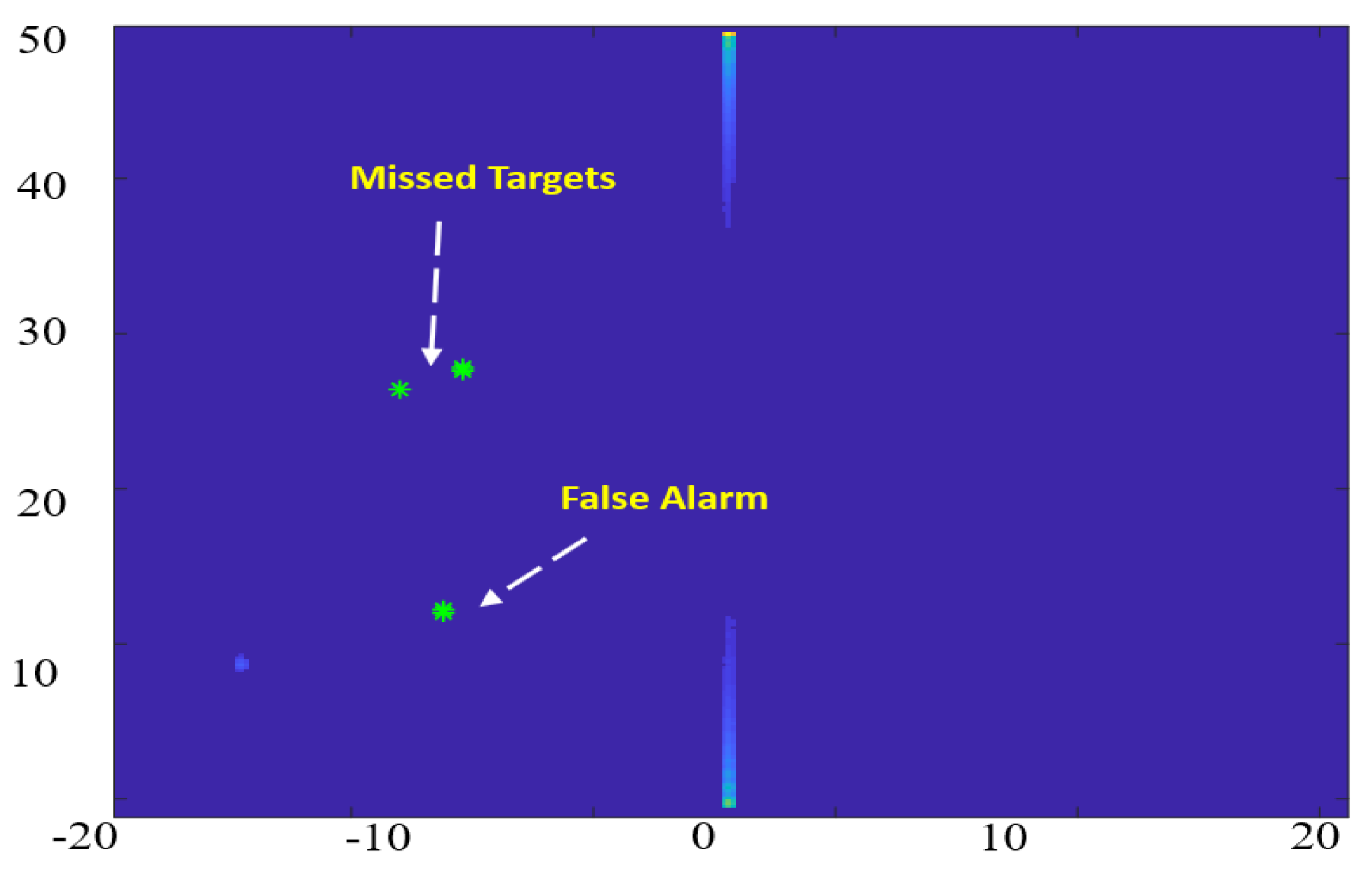
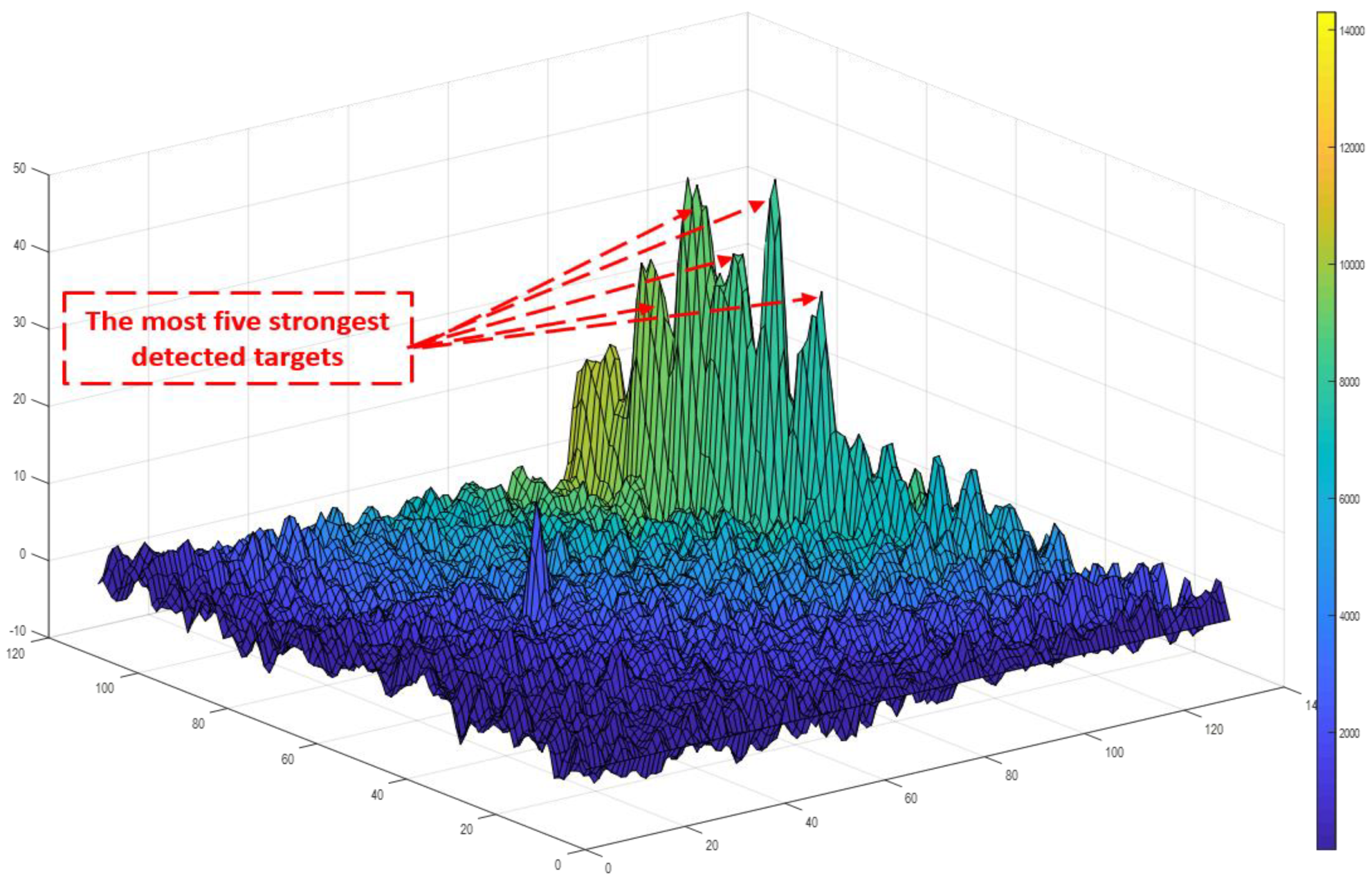
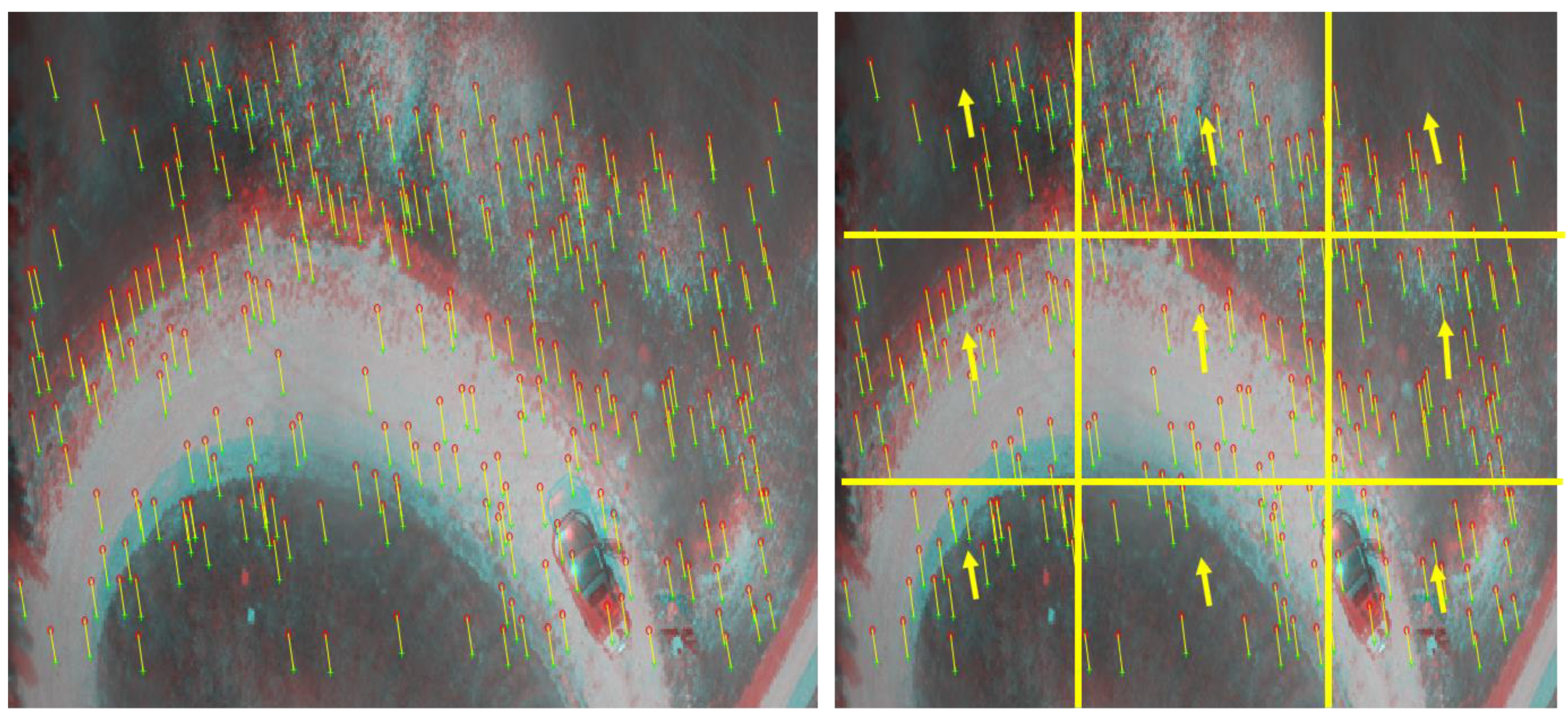
2.1.2. Target Detection and Data Extraction
2.2. Enhanced Moncular Visual Odometry
2.2.1. Monocular Visual Odometry
2.2.2. Velocity Compensation
2.3. Data Fusion
2.3.1. Prediction Model
2.3.2. Observation Model
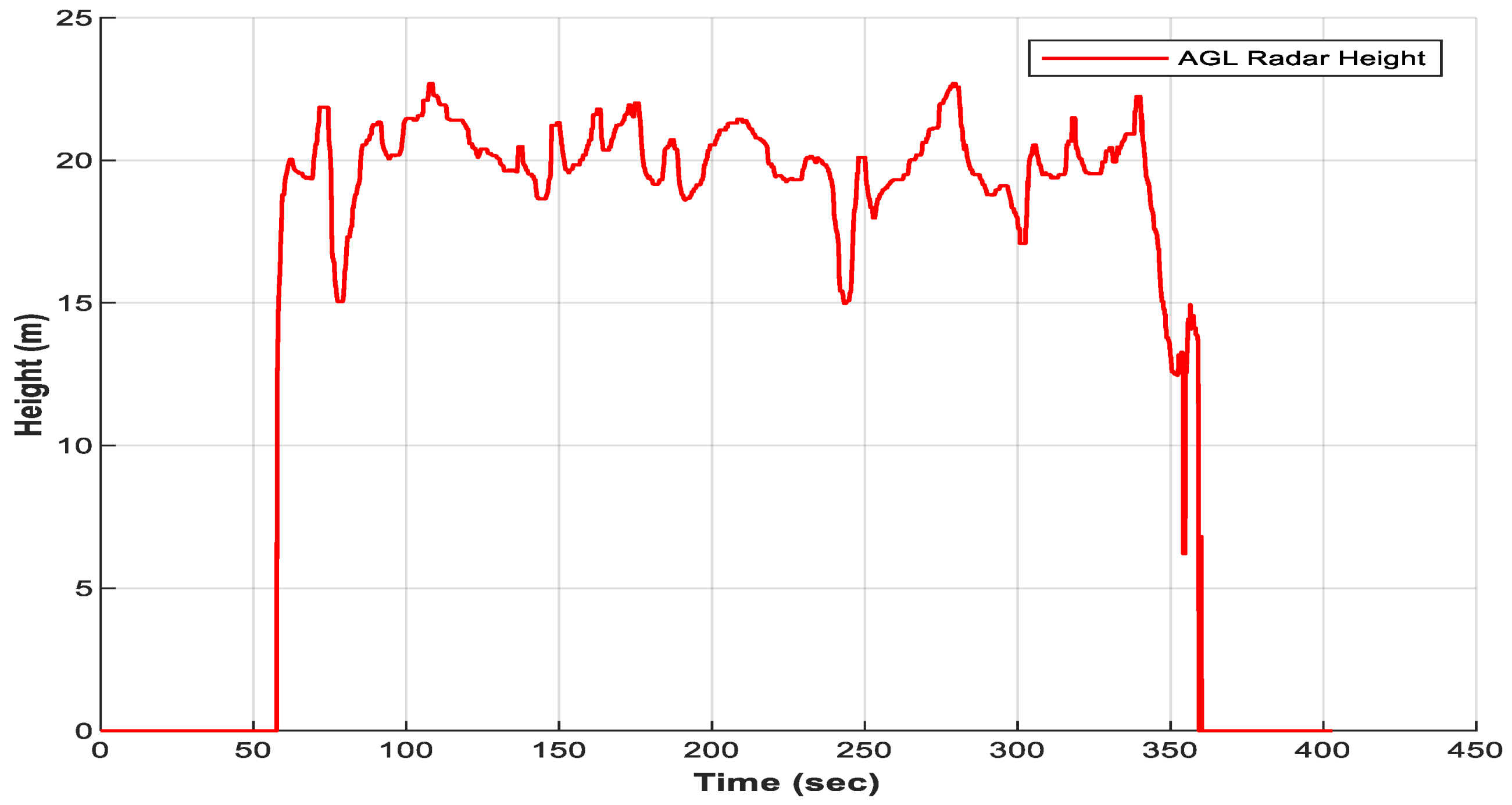
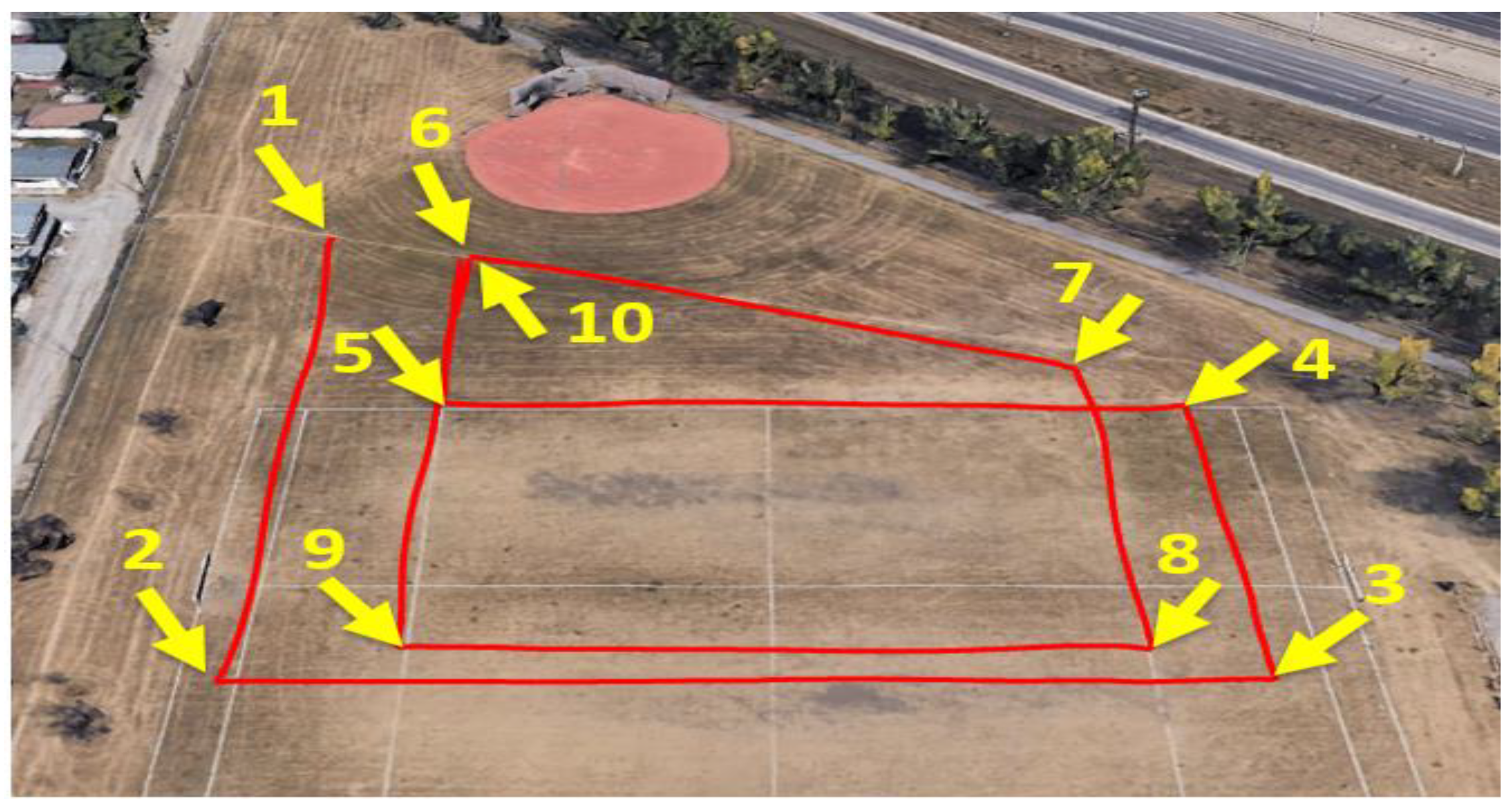
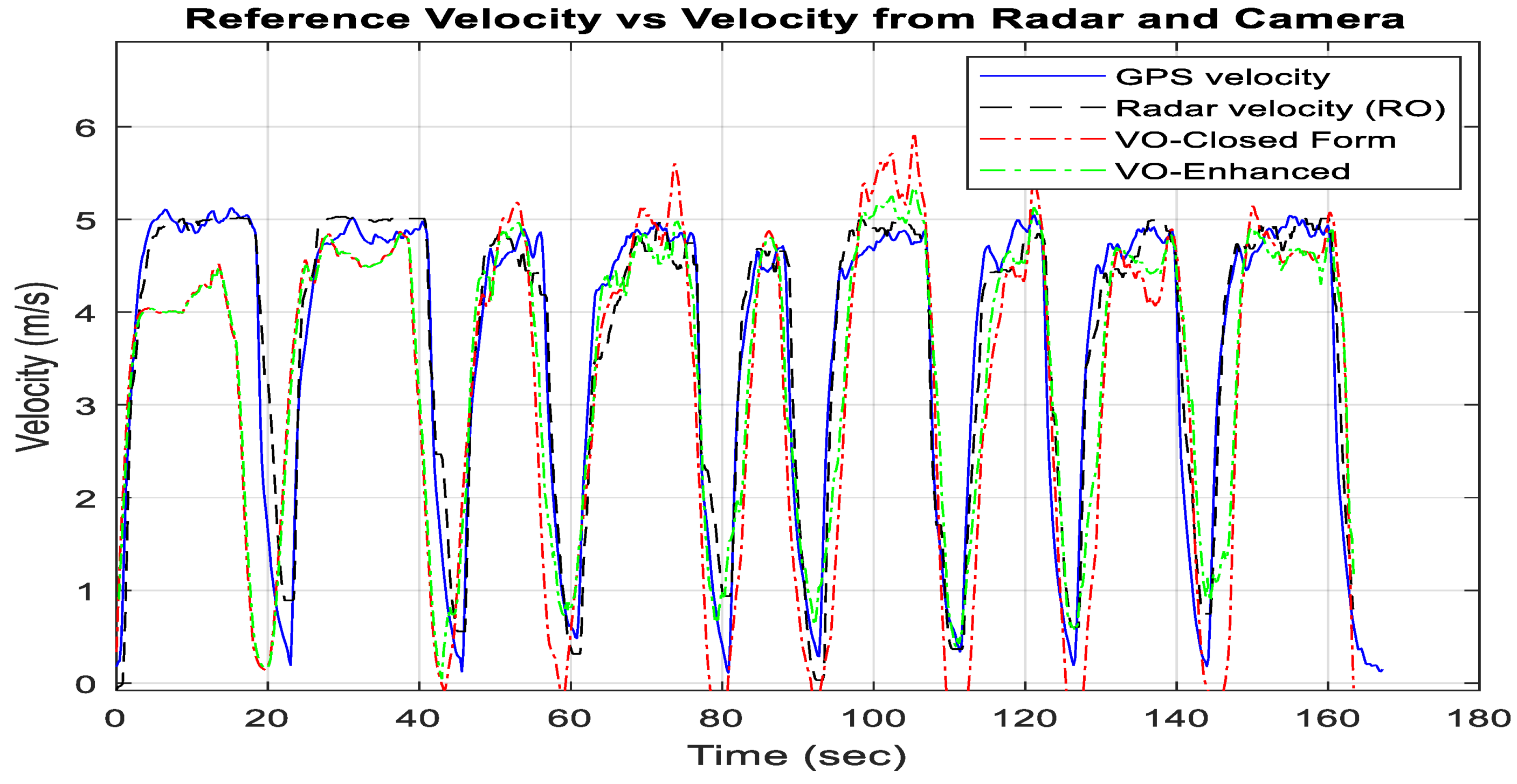
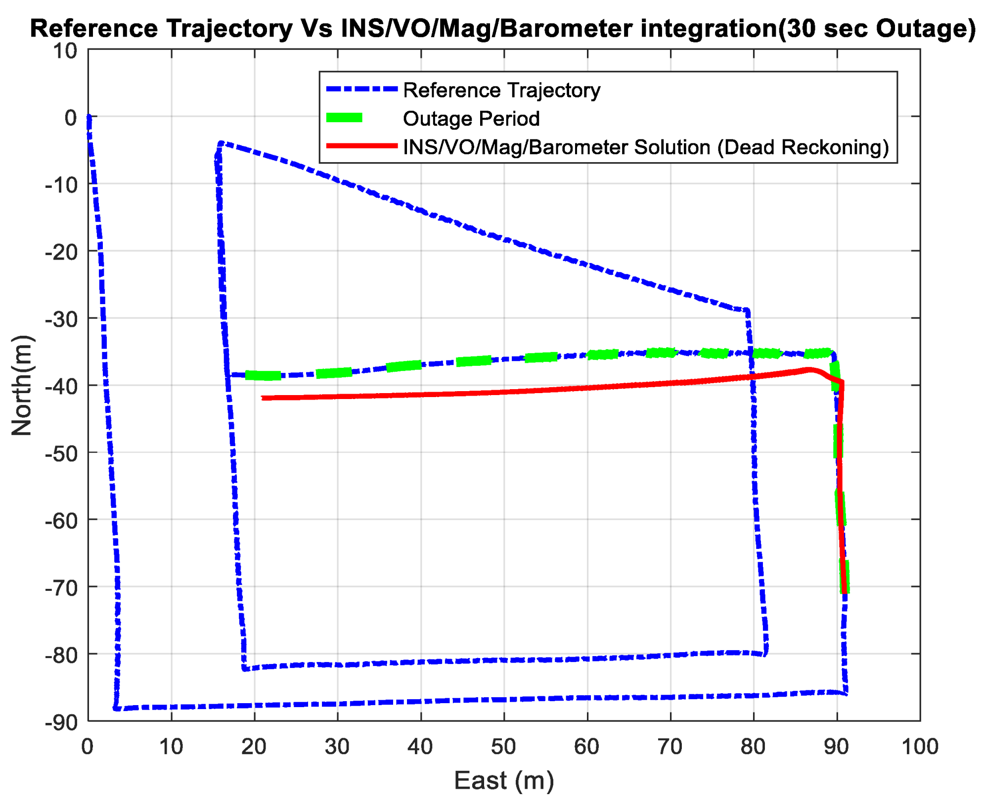
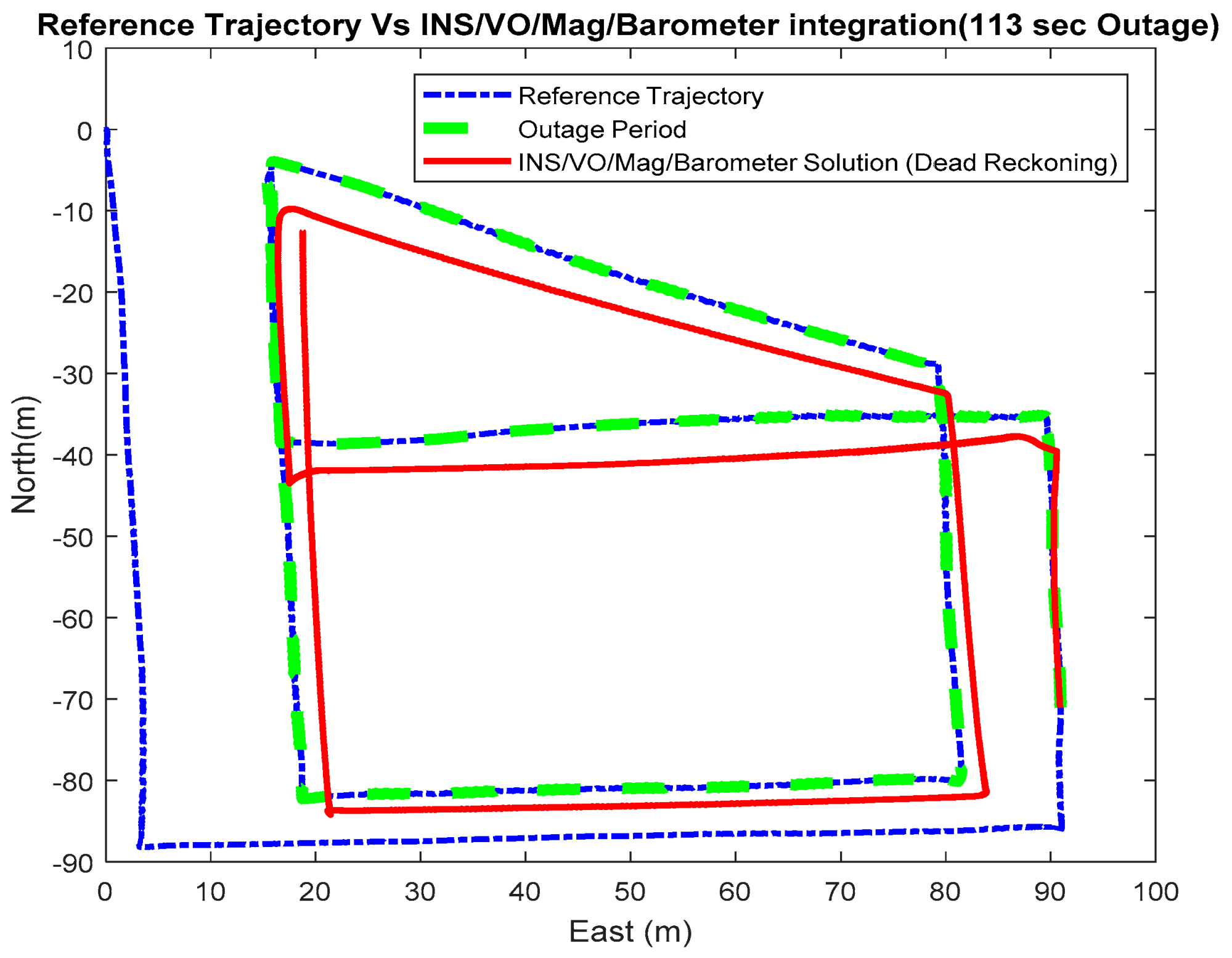
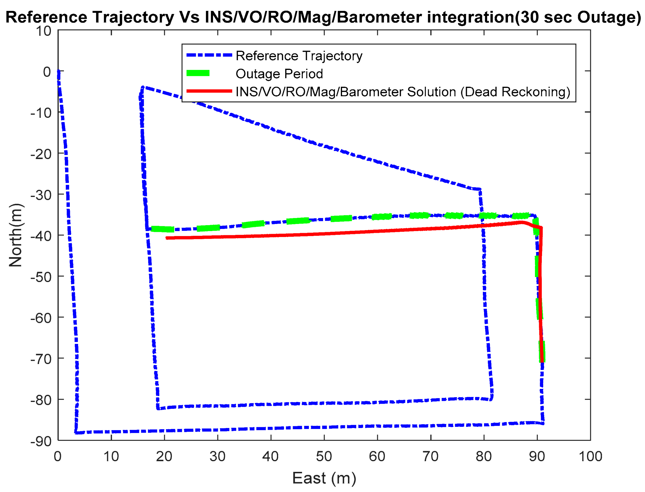
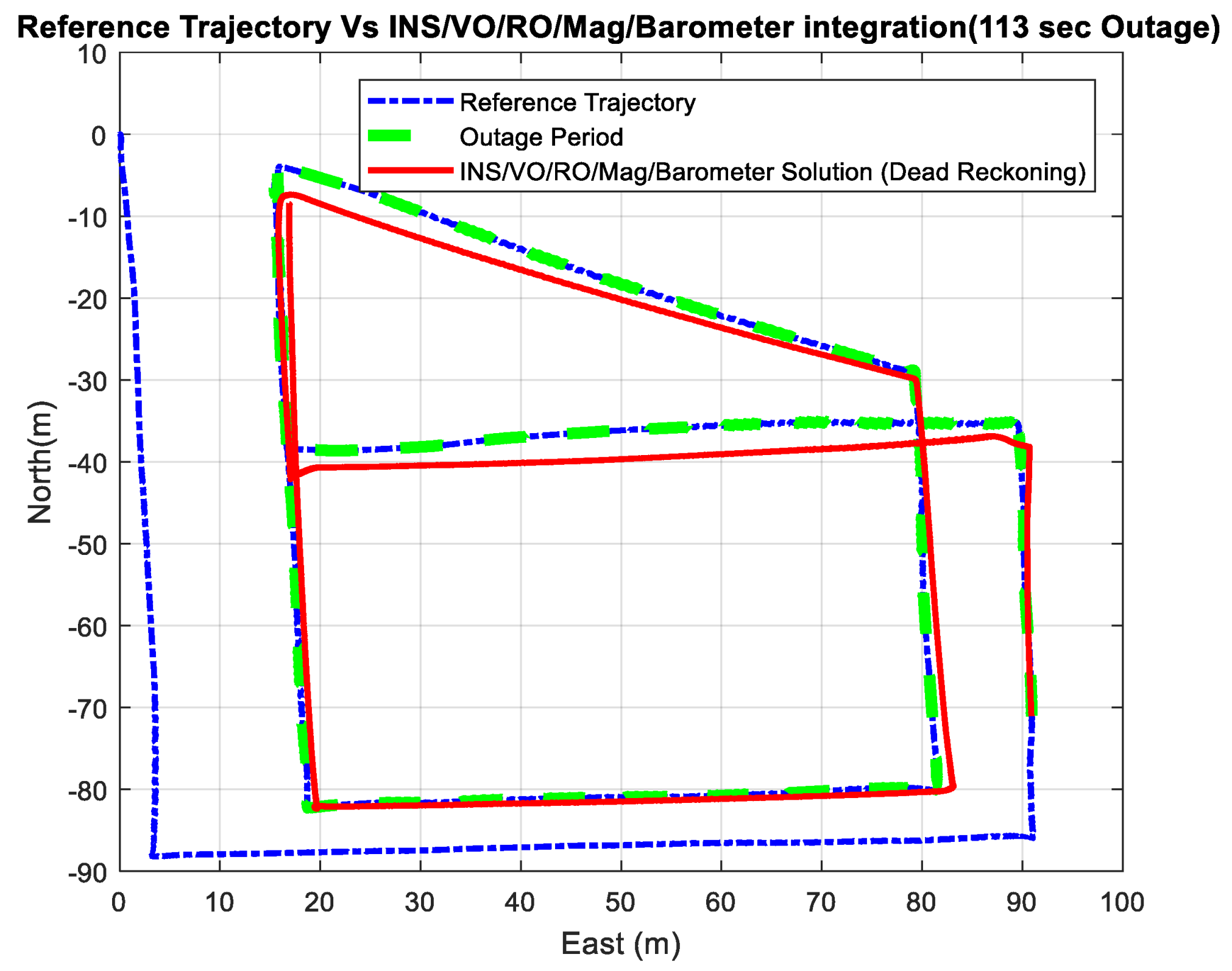
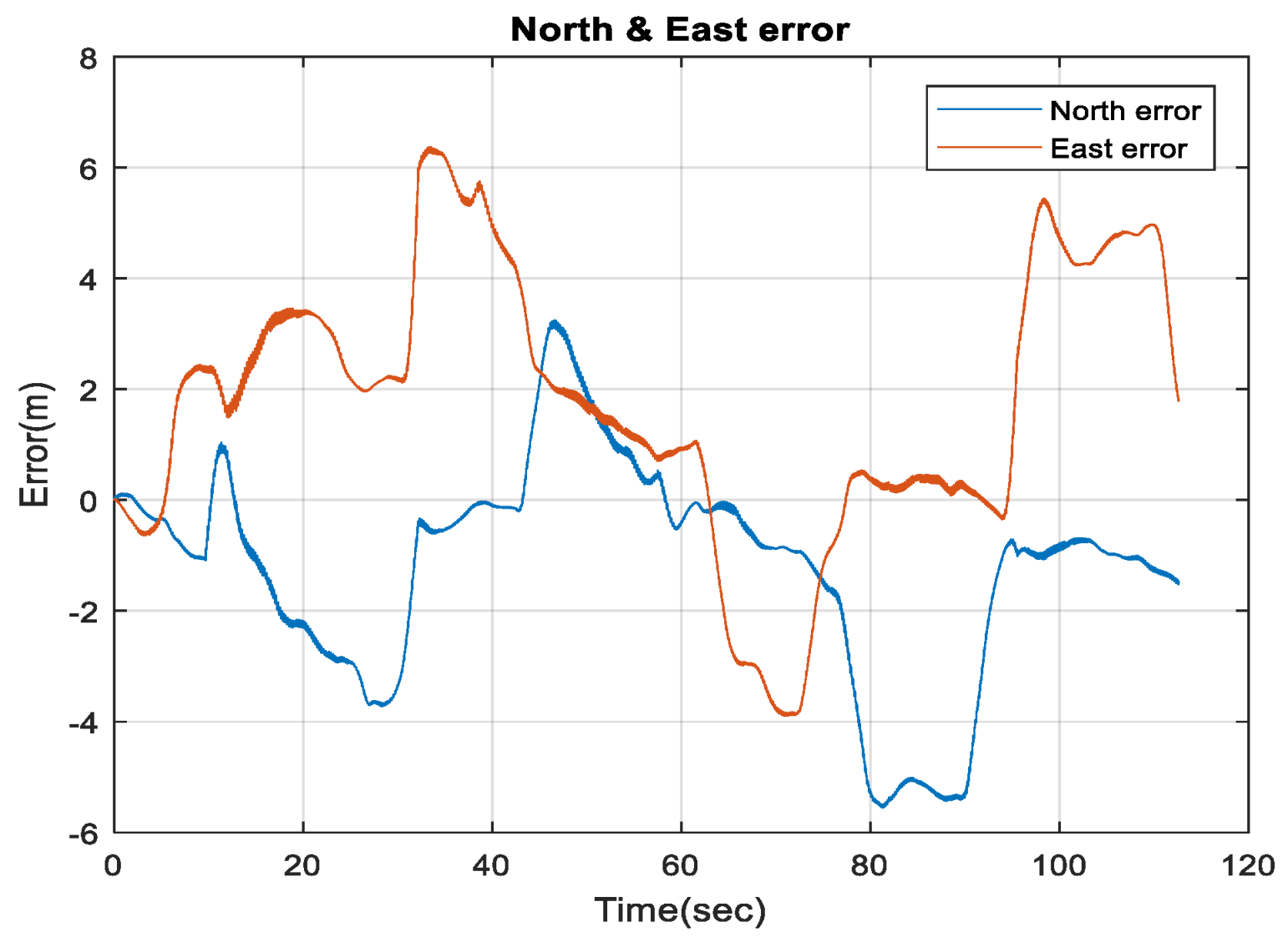
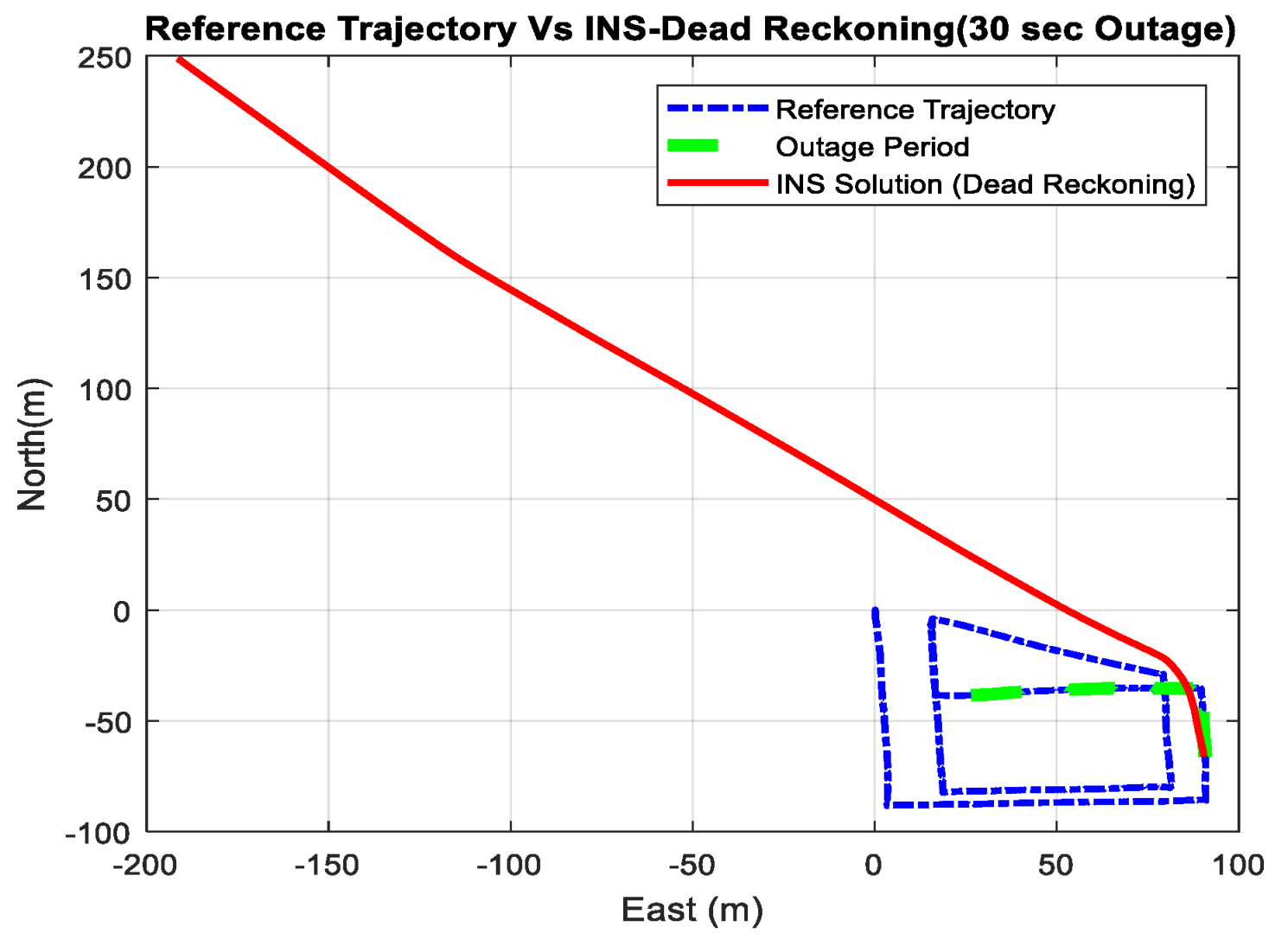
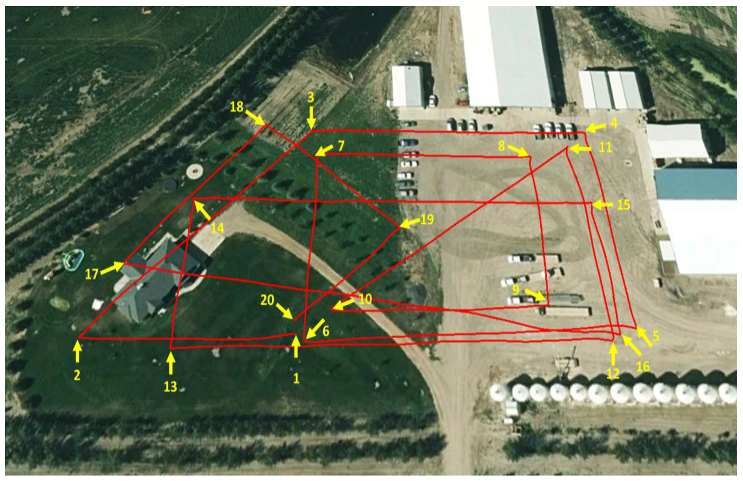
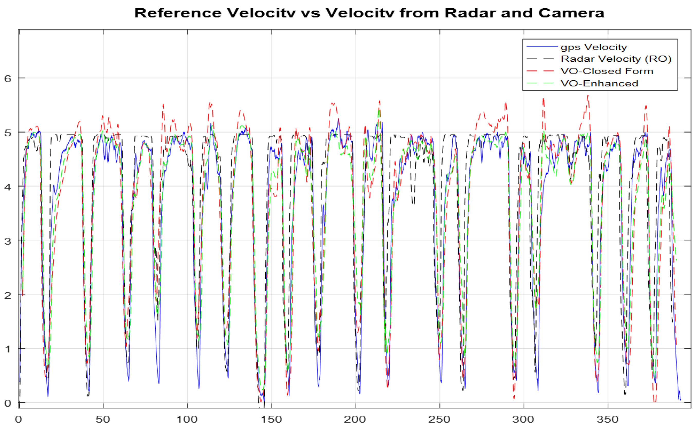
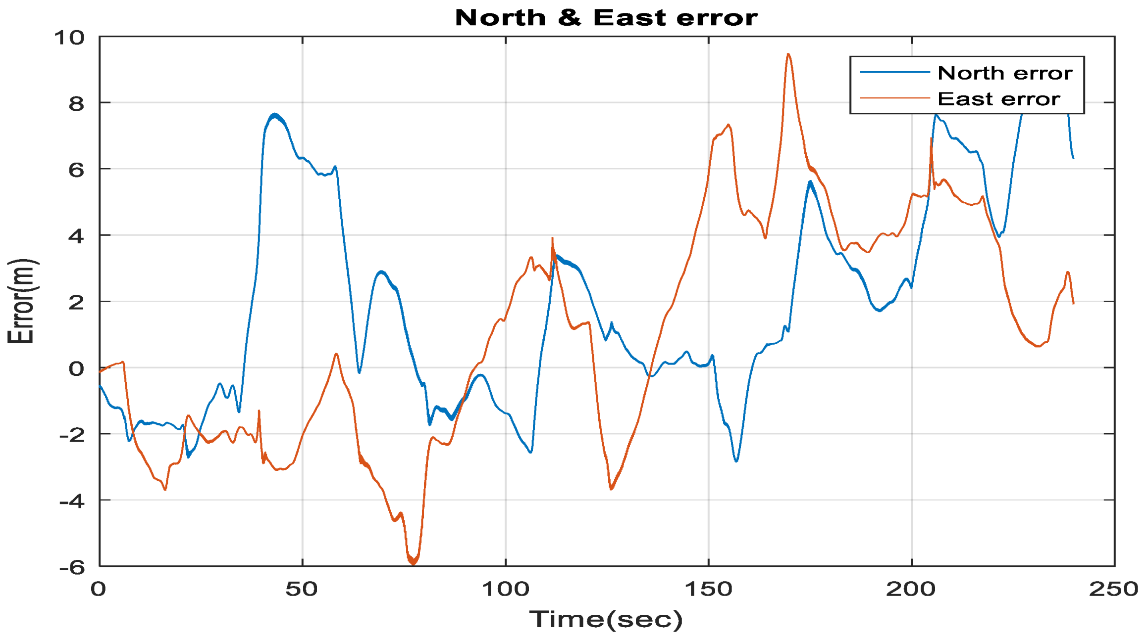
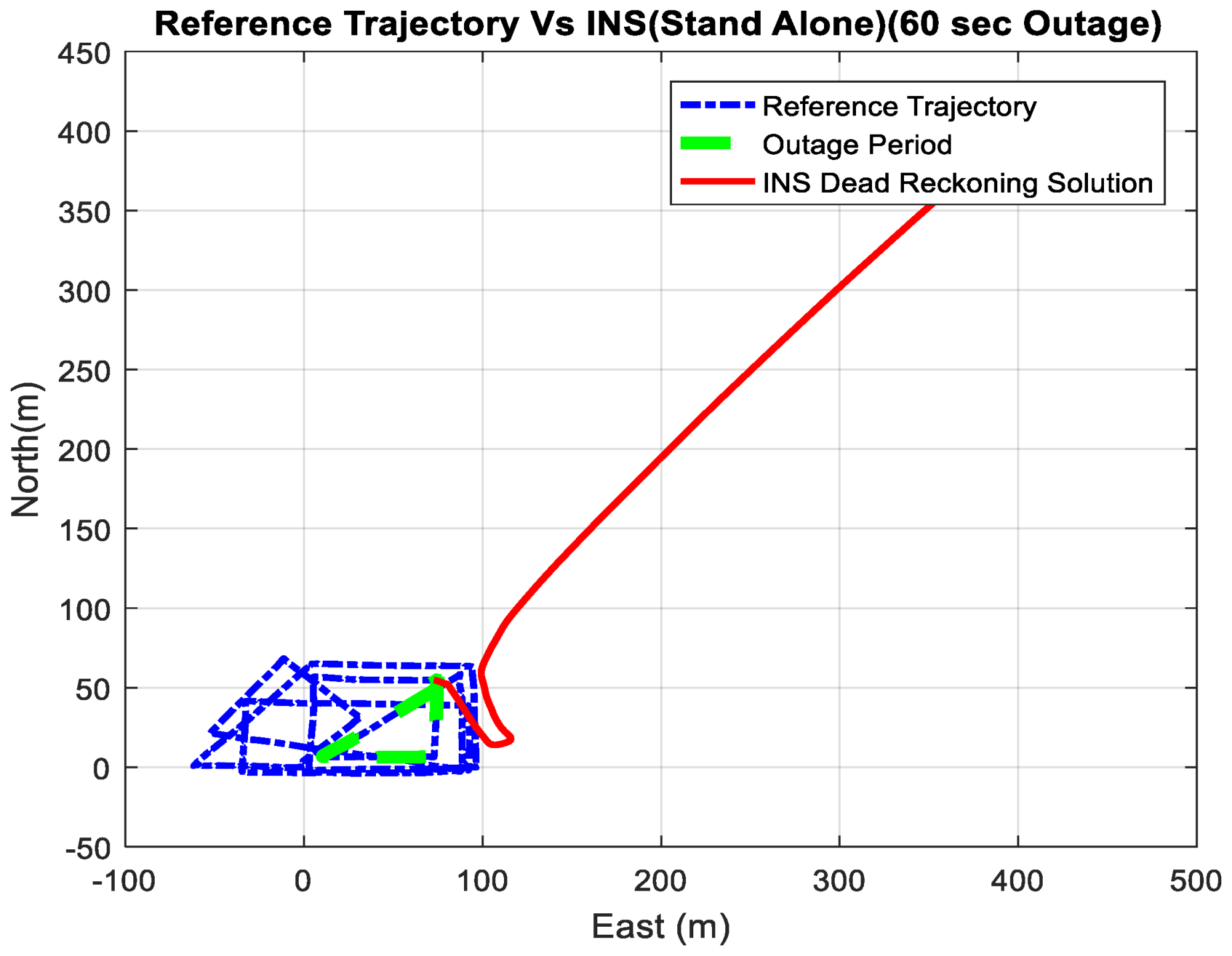
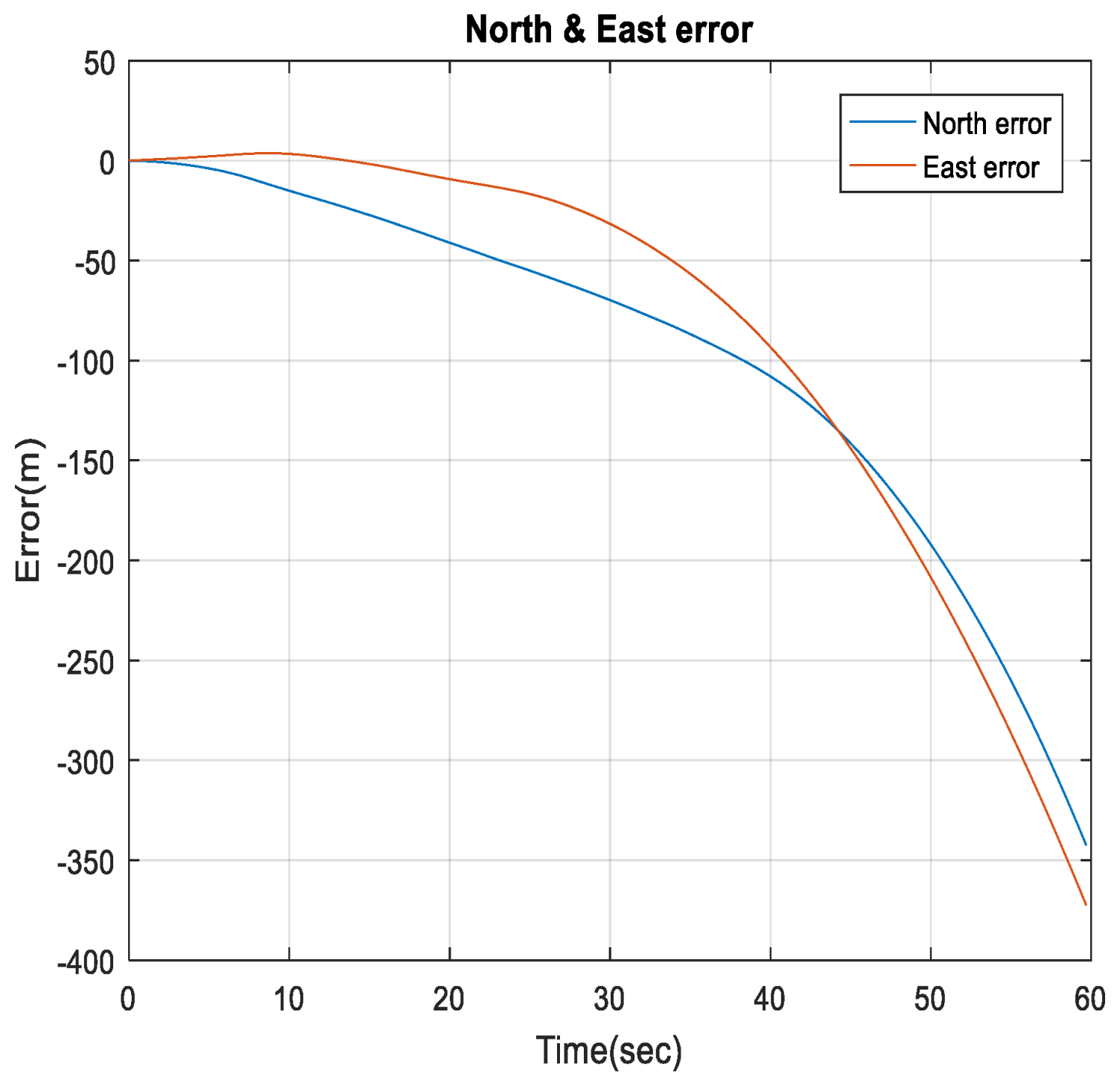
3. Experimental Results
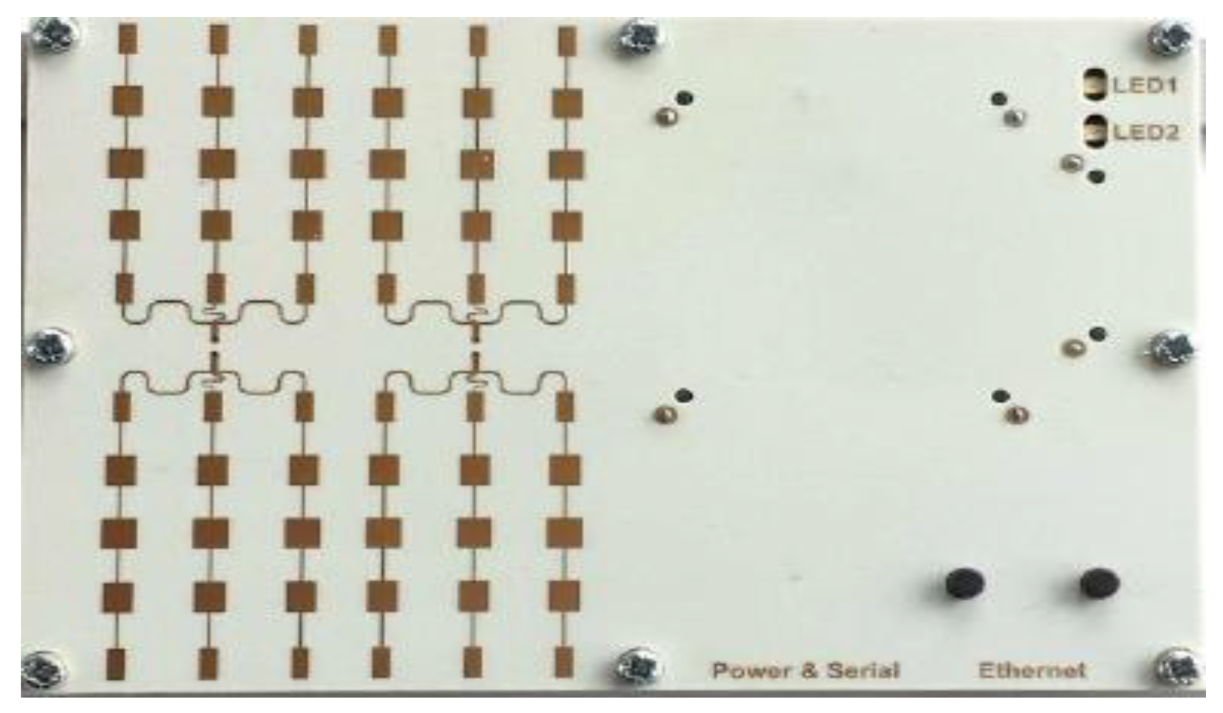
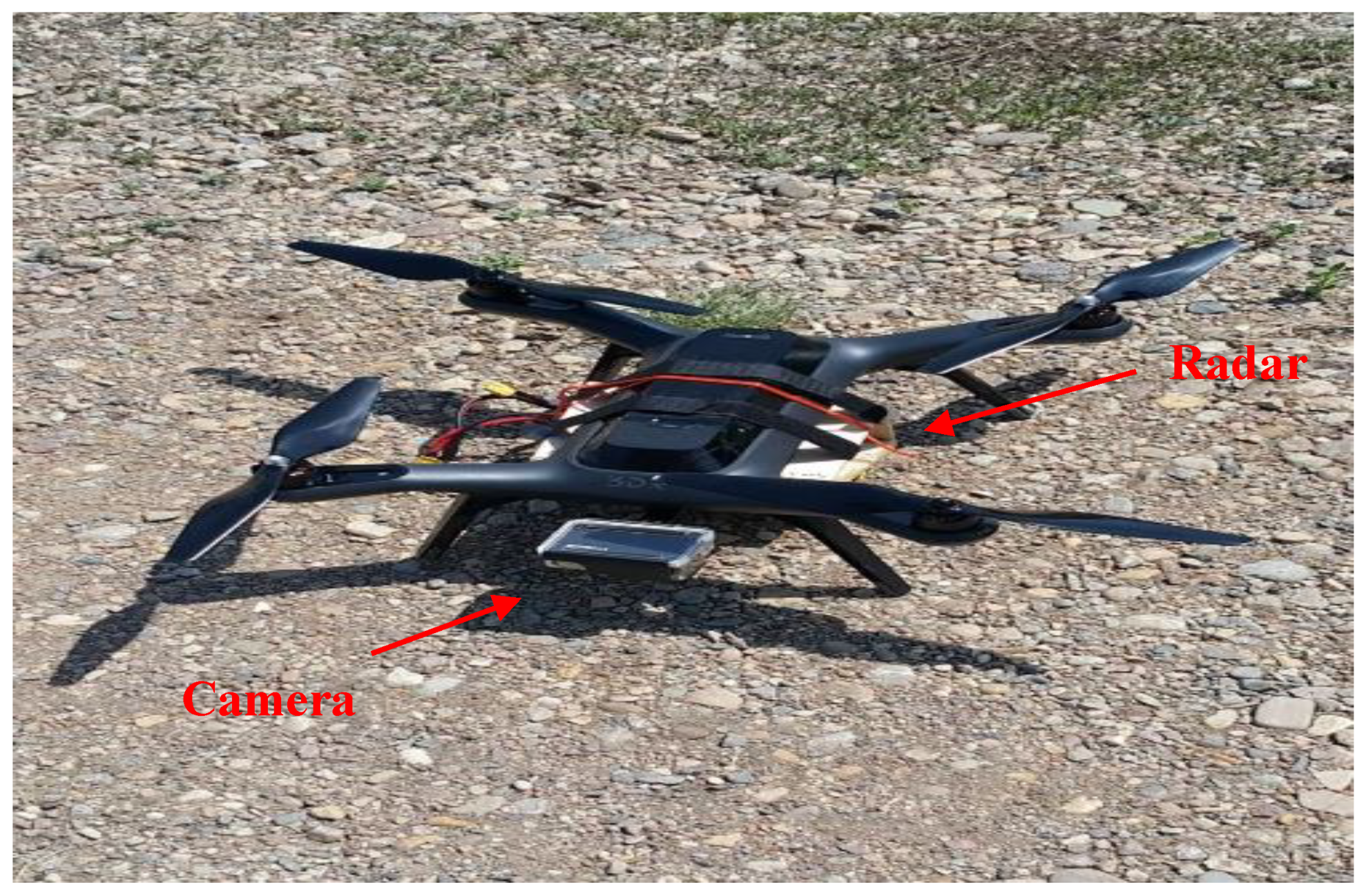
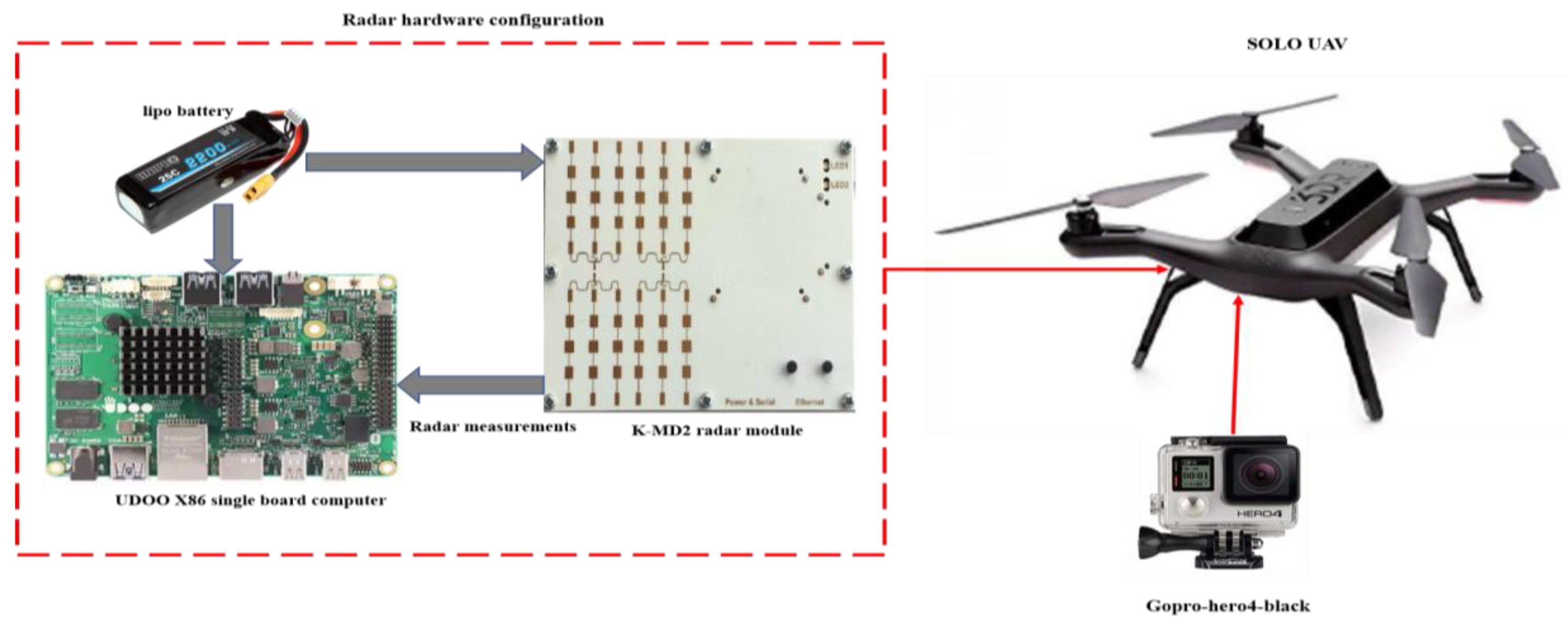
3.1. Hardware Setup
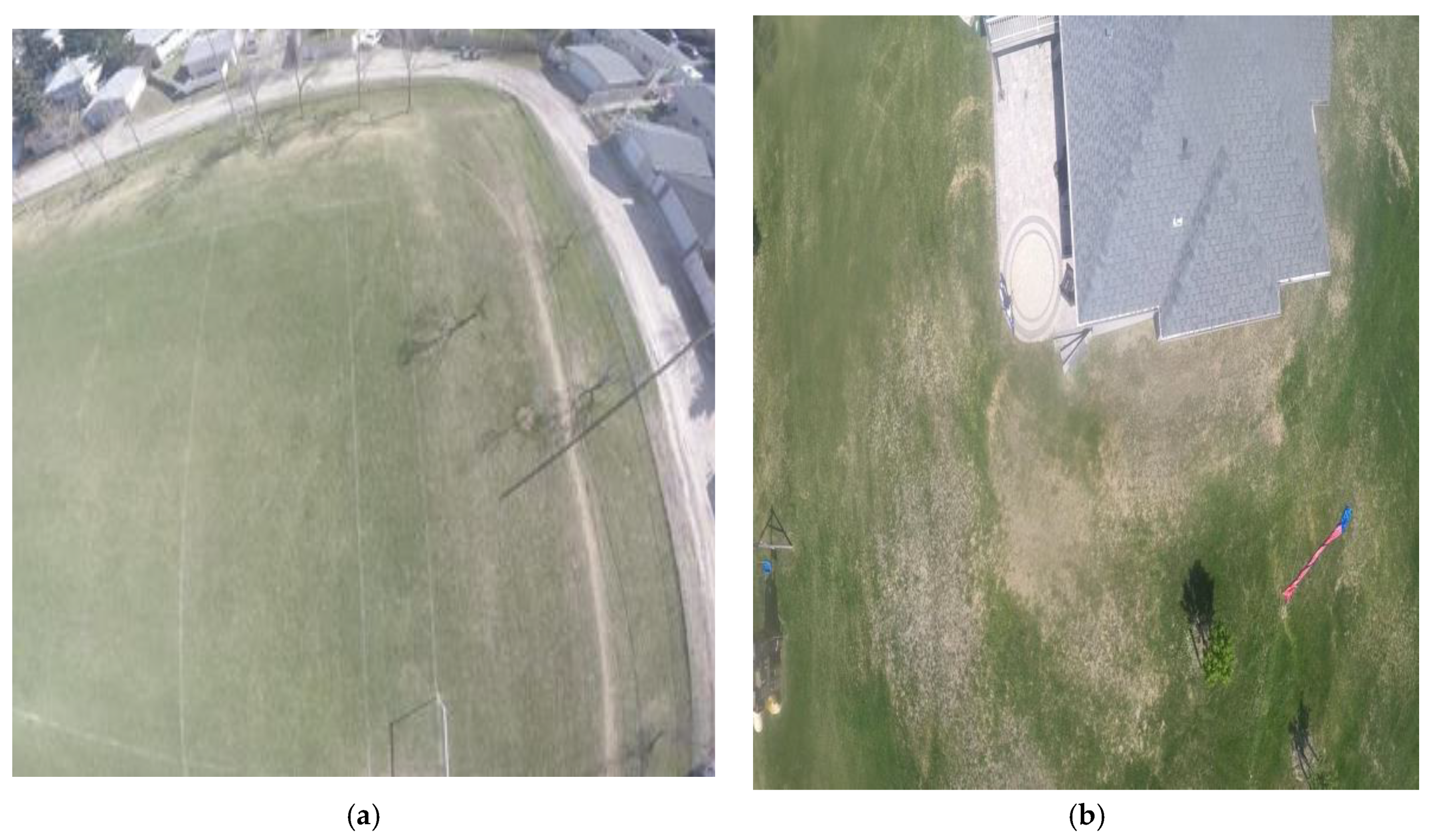
3.2.1. First Experiment
3.2.2. Second Experiment
4. Conclusions
Author Contributions
Funding
Acknowledgments
Conflicts of Interest
References
- Achtelik, M.; Weiss, S.; Siegwart, R. Onboard IMU and monocular vision based control for MAVs in unknown in- and outdoor environments. In Proceedings of the 2011 IEEE International Conference on Robotics and Automation, Shanghai, China, 9–13 May 2011; pp. 3056–3063. [Google Scholar]
- Blösch, M.; Weiss, S.; Scaramuzza, D.; Siegwart, R. Vision based MAV navigation in unknown and unstructured environments. In Proceedings of the 2010 IEEE International Conference on Robotics and Automation, Anchorage, AK, USA, 3–7 May 2010; pp. 21–28. [Google Scholar]
- Mostafa, M.; Moussa, A.; El-Sheimy, N.; Sesay, A.A. Optical Flow Based Approach for Vision Aided Inertial Navigation Using Regression Trees. In Proceedings of the 2017 International Technical Meeting of The Institute of Navigation, Monterey, CA, USA, 30 January–2 February 2017; pp. 856–865. [Google Scholar]
- Civera, J.; Davison, A.J.; Montiel, J.M. Dimensionless Monocular SLAM. In Proceedings of the 3rd Iberian Conference on Pattern Recognition and Image Analysis, Part II, Girona, Spain, 6–8 June 2007; pp. 412–419. [Google Scholar]
- Davison, A.J.; Reid, I.D.; Molton, N.D.; Stasse, O. MonoSLAM: Real-Time Single Camera SLAM. IEEE Trans. Pattern Anal. Mach. Intell. 2007, 29, 1052–1067. [Google Scholar] [CrossRef] [PubMed] [Green Version]
- Huang, K.-C.; Tseng, S.-H.; Mou, W.-H.; Fu, L.-C. Simultaneous localization and scene reconstruction with monocular camera. In Proceedings of the 2012 IEEE International Conference on Robotics and Automation, Saint Paul, MN, USA, 14–18 May 2012; pp. 2102–2107. [Google Scholar]
- Klein, G.; Murray, D. Parallel Tracking and Mapping for Small AR Workspaces. In Proceedings of the 2007 6th IEEE and ACM International Symposium on Mixed and Enhanced Reality, Nara, Japan, 13–16 November 2007; pp. 225–234. [Google Scholar]
- Scaramuzza, D.; Fraundorfer, F.; Siegwart, R. Real-time monocular visual odometry for on-road vehicles with 1-point RANSAC. In Proceedings of the 2009 IEEE International Conference on Robotics and Automation, Kobe, Japan, 12–17 May 2009; pp. 4293–4299. [Google Scholar]
- Strasdat, H.; Montiel, J.M.M.; Davison, A.J. Real-time monocular SLAM: Why filter? In Proceedings of the 2010 IEEE International Conference on Robotics and Automation, Anchorage, AK, USA, 3–7 May 2010; pp. 2657–2664. [Google Scholar]
- Weiss, S.; Scaramuzza, D.; Siegwart, R. Monocular-SLAM—Based Navigation for Autonomous Micro Helicopters in GPS-denied Environments. J. Field Robot 2011, 28, 854–874. [Google Scholar] [CrossRef]
- Eynard, D.; Vasseur, P.; Demonceaux, C.; Frémont, V. UAV altitude estimation by mixed stereoscopic vision. In Proceedings of the 2010 IEEE/RSJ International Conference on Intelligent Robots and Systems, Taipei, Taiwan, 18–22 October 2010; pp. 646–651. [Google Scholar]
- Lategahn, H.; Stiller, C. City GPS using stereo vision. In Proceedings of the 2012 IEEE International Conference on Vehicular Electronics and Safety (ICVES 2012), Istanbul, Turkey, 24–27 July 2012; pp. 1–6. [Google Scholar]
- Rehder, J.; Gupta, K.; Nuske, S.; Singh, S. Global pose estimation with limited GPS and long range visual odometry. In Proceedings of the 2012 IEEE International Conference on Robotics and Automation, Saint Paul, MN, USA, 14–18 May 2012; pp. 627–633. [Google Scholar]
- Bryson, M.; Johnson-Roberson, M.; Sukkarieh, S. Airborne smoothing and mapping using vision and inertial sensors. In Proceedings of the 2009 IEEE International Conference on Robotics and Automation, Kobe, Japan, 12–17 May 2009; pp. 2037–2042. [Google Scholar]
- Karamat, T.B.; Lins, R.G.; Givigi, S.N.; Noureldin, A. Novel EKF-Based Vision/Inertial System Integration for Improved Navigation. IEEE Trans. Instrum. Meas. 2018, 67, 116–125. [Google Scholar] [CrossRef]
- Feuerstein, E.; Safran, H.; James, P.N. Inaccuracies in Doppler Radar Navigation Systems Due to Terrain Directivity Efects, Nonzero Beamwidths and Eclipsing. IEEE Trans. Aerosp. Navig. Electron. 1964, 2, 101–111. [Google Scholar] [CrossRef]
- Kauffman, K.; Raquet, J.; Morton, Y.; Garmatyuk, D. Real-Time UWB-OFDM Radar-Based Navigation in Unknown Terrain. IEEE Trans. Aerosp. Electron. Syst. 2013, 49, 1453–1466. [Google Scholar] [CrossRef]
- ARTECH HOUSE USA: Design and Analysis of Modern Tracking Systems. Available online: http://us.artechhouse.com/Design-and-Analysis-of-Modern-Tracking-Systems-P170.aspx (accessed on 1 November 2017).
- Quist, E.B.; Beard, R.W. Radar odometry on fixed-wing small unmanned aircraft. IEEE Trans. Aerosp. Electron. Syst. 2016, 52, 396–410. [Google Scholar] [CrossRef]
- Duda, R.O.; Hart, P.E. Use of the Hough transformation to detect lines and curves in pictures. Commun. ACM 1972, 15, 11–15. [Google Scholar] [CrossRef] [Green Version]
- Quist, E.B.; Niedfeldt, P.C.; Beard, R.W. Radar odometry with recursive-RANSAC. IEEE Trans. Aerosp. Electron. Syst. 2016, 52, 1618–1630. [Google Scholar] [CrossRef]
- Quist, E.B.; Beard, R. Radar odometry on small unmanned aircraft. In Proceedings of the AIAA Guidance, Navigation, and Control (GNC) Conference, Boston, MA, USA, 19–22 August 2013; p. 4698. [Google Scholar]
- Scannapieco, A.F.; Renga, A.; Fasano, G.; Moccia, A. Ultralight radar sensor for autonomous operations by micro-UAS. In Proceedings of the 2016 International Conference on Unmanned Aircraft Systems (ICUAS), Arlington, VA, USA, 7–10 June 2016; pp. 727–735. [Google Scholar]
- Rohling, H. Radar CFAR Thresholding in Clutter and Multiple Target Situations. IEEE Trans. Aerosp. Electron. Syst. 1983, 19, 608–621. [Google Scholar] [CrossRef]
- Banerjee, S.; Roy, A. Linear Algebra and Matrix Analysis for Statistics; CRC Press: Boca Raton, FL, USA, 2014. [Google Scholar]
- Vadlamani, A.K.; de Haag, M.U. Improved downward-looking terrain database integrity monitor and terrain navigation. In Proceedings of the 2004 IEEE Aerospace Conference Proceedings (IEEE Cat. No. 04TH8720), Big Sky, MT, USA, 6–13 March 2004; Volume 3, p. 1607. [Google Scholar]
- Vadlamani, A.K.; de Haag, M.U. Flight test results of loose integration of dual airborne laser scanners (DALS)/INS. In Proceedings of the 2008 IEEE/ION Position, Location and Navigation Symposium, Monterey, CA, USA, 5–8 May 2008. [Google Scholar]
- Wojtkiewicz, A.; Misiurewicz, J.; Nalecz, M.; Jedrzejewski, K.; Kulpa, K. Two-dimensional signal processing in FMCW radars. Proc. XX KKTOiUE 1997, 475–480. [Google Scholar]
- Skolnik, M.I. Introduction to Radar Systems, 2nd ed.; McGraw-Hill: New York, NY, USA, 1980. [Google Scholar]
- Bay, H.; Ess, A.; Tuytelaars, T.; van Gool, L. Speeded-Up Robust Features (SURF). Comput. Vis. Image Underst. 2008, 110, 346–359. [Google Scholar] [CrossRef] [Green Version]
- Shin, E.H. Estimation Techniques for Low-Cost Inertial Navigation. Ph.D. Thesis, University of Calgary, Calgary, AB, Canada, 2005. [Google Scholar]
- Noureldin, A.; Karamat, T.; Georgy, J. Fundamentals of Inertial Navigation, Satellite-Based Positioning, and Their Integration; Springer: Heidelberg, Germany; New York, NY, USA; Dordrecht, The Netherlands; London, UK, 2013. [Google Scholar]
- Shin, E.H. Accuracy Improvement of Low Cost INS/GPS for Land Applications; University of Calgary: Calgary, AB, Canada, 2001. [Google Scholar]


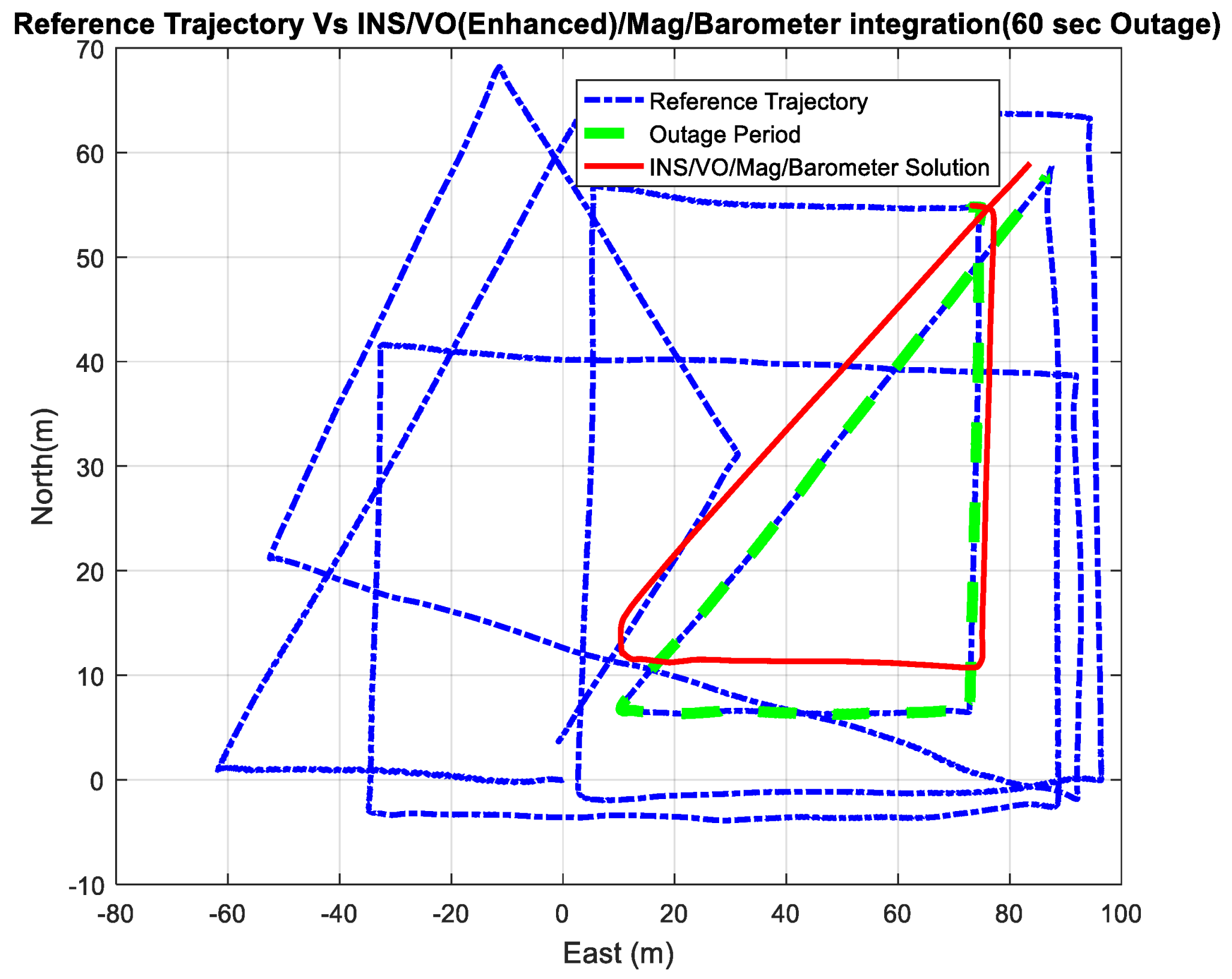
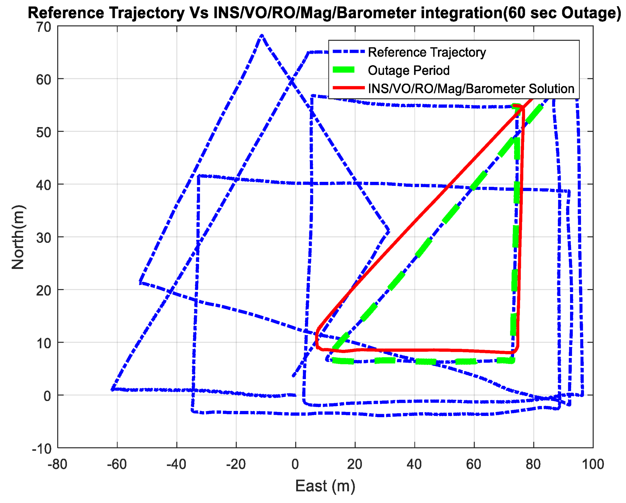
| Symbol | Symbol | Outage [30 s] | Outage [113 s] |
|---|---|---|---|
| North error [m] | INS | 38.06 | 2002 |
| Enhanced VO | 1.52 | 2.64 | |
| Integrated system | 0.85 | 1.87 | |
| East error [m] | INS | 54.59 | 1436 |
| Enhanced VO | 0.85 | 4.02 | |
| Integrated system | 0.98 | 2.47 | |
| Height error [m] | INS | 5.08 | 221 |
| Enhanced VO | 0.25 | 0.61 | |
| Integrated system | 0.45 | 0.74 | |
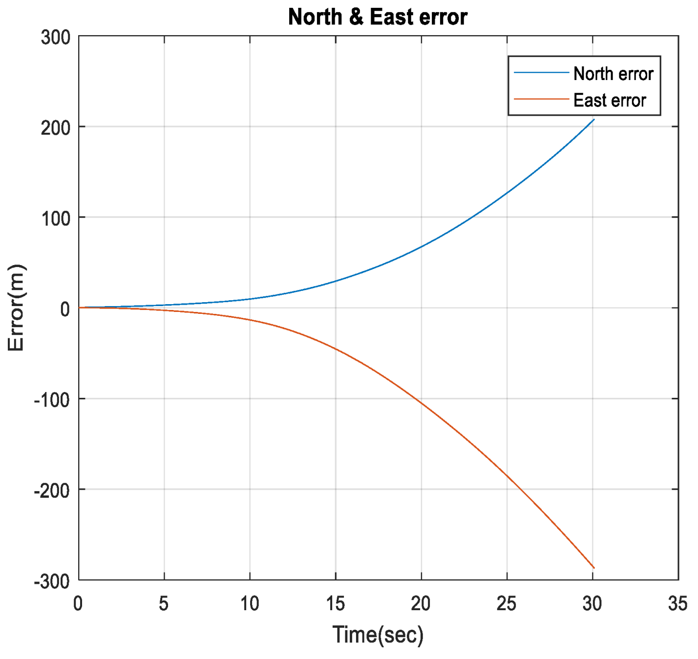
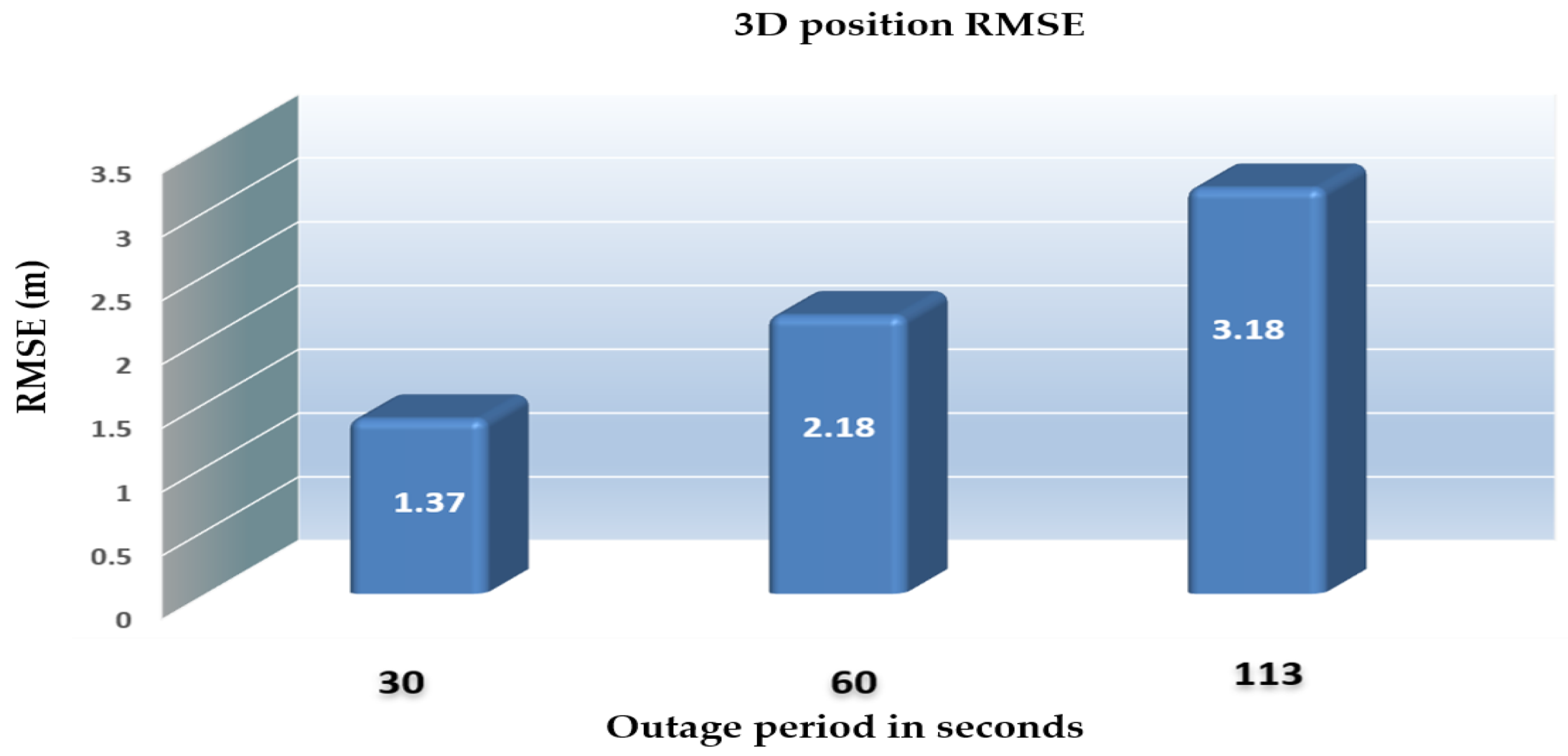
| 3D Position error [m] | INS | 66.74 | 2473 |
| Enhanced VO | 1.75 | 4.84 | |
| Integrated system | 1.37 | 3.18 | |
| Enhancement percentage from the INS% | |||
| Enhanced VO | 97.36 | 99.80 | |
| Integrated system | 97.94 | 99.87 |
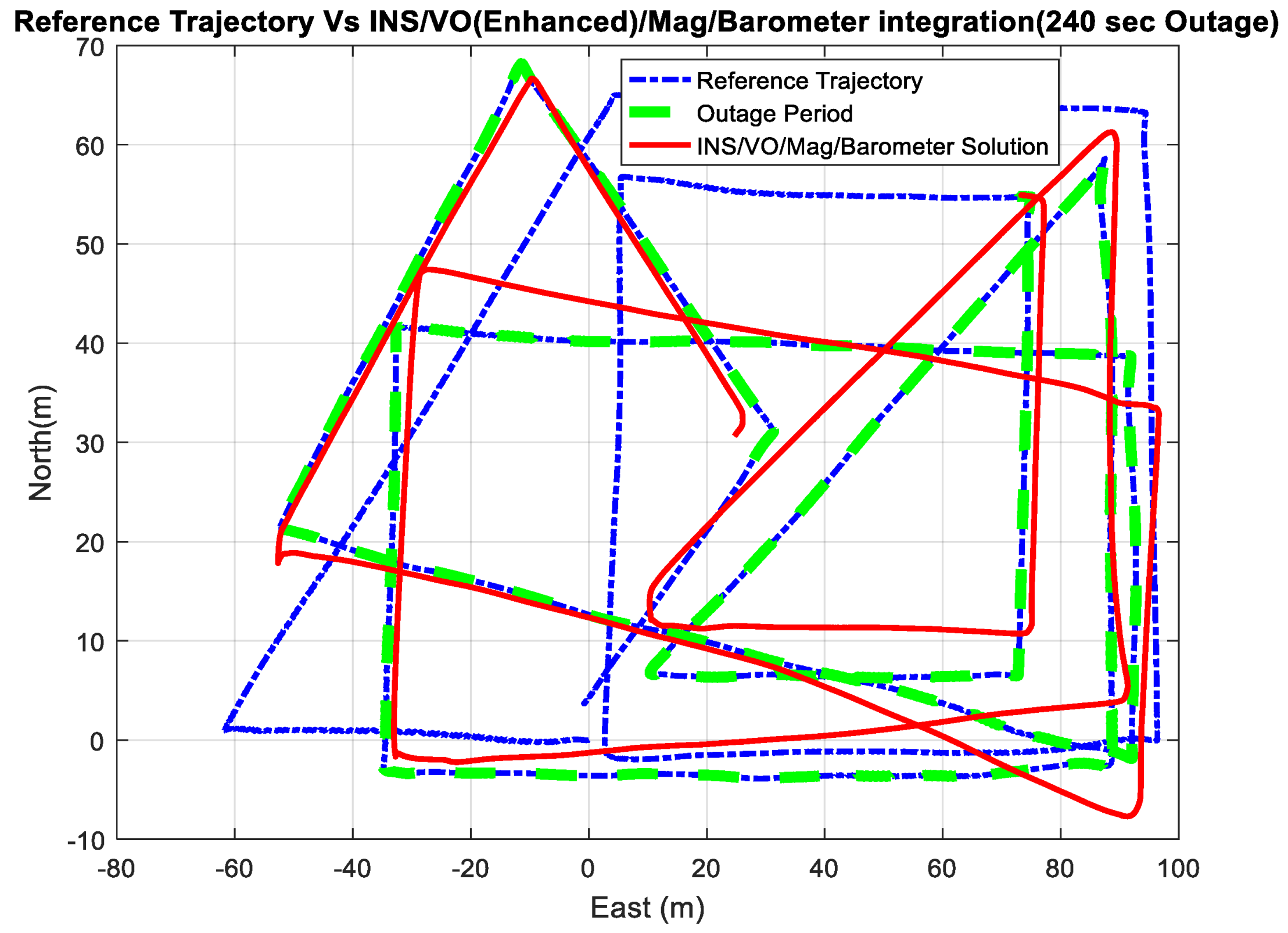
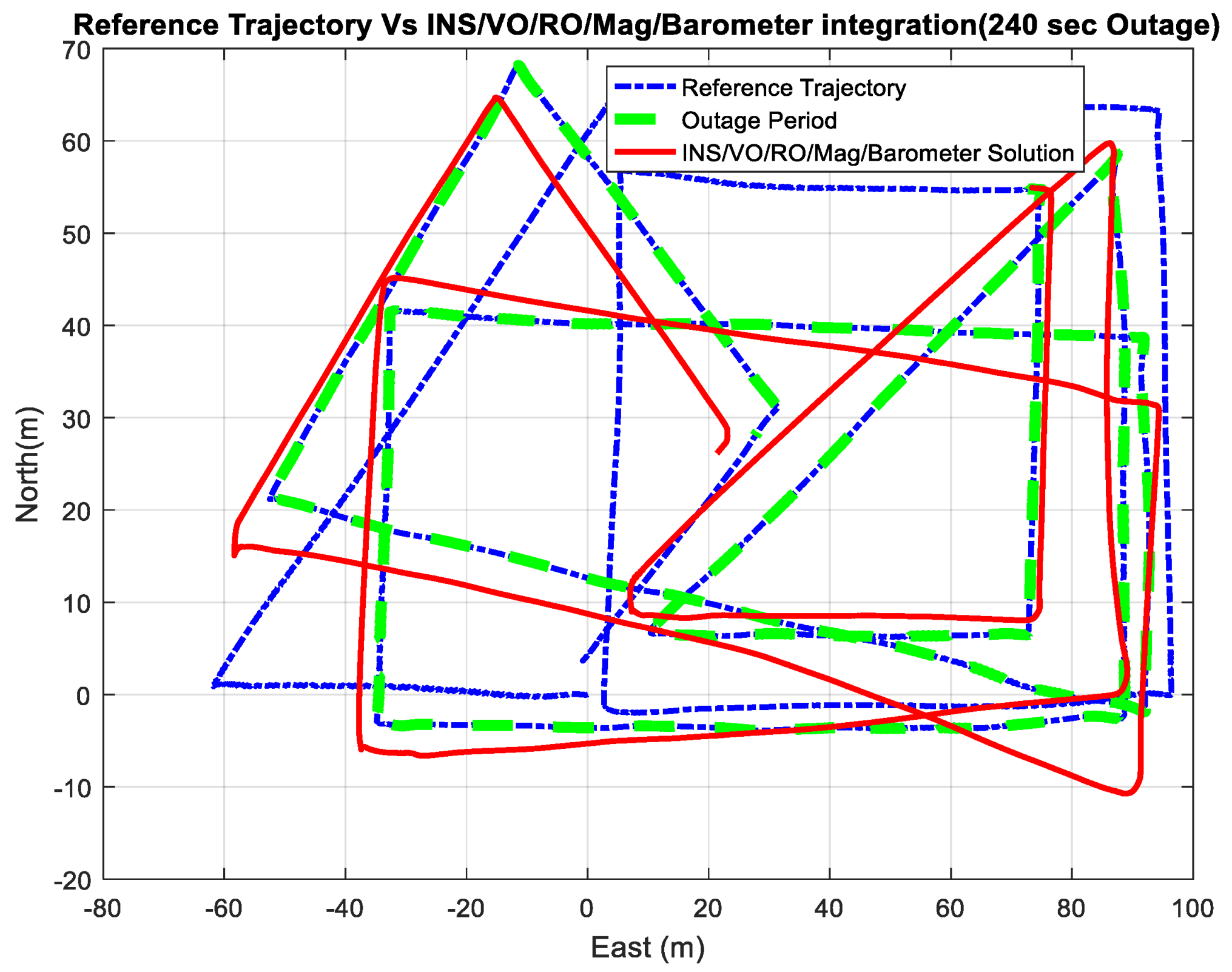
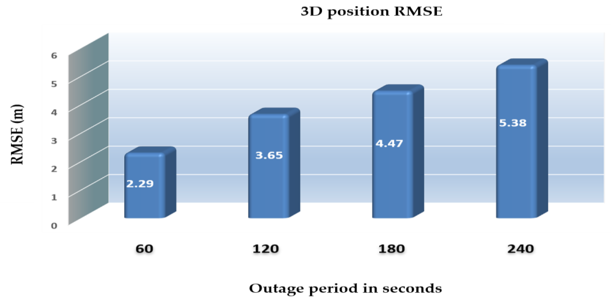
| Symbol | Symbol | Outage [60 s] | Outage [240 s] |
|---|---|---|---|
| North error [m] | INS | 50.95 | 1233 |
| Enhanced VO | 1.29 | 2.63 | |
| Integrated system | 1.57 | 2.75 | |
| East error [m] | INS | 52.76 | 5680 |
| Enhanced VO | 1.63 | 2.85 | |
| Integrated system | 0.85 | 2.81 | |
| Height error [m] | INS | 12.45 | 878 |
| Enhanced VO | 1.35 | 3.53 | |
| Integrated system | 1.44 | 3.68 | |
| 3D Position error [m] | INS | 74.39 | 5878 |
| Enhanced VO | 2.47 | 5.24 | |
| Integrated system | 2.29 | 5.38 | |
| Enhancement percentage from the INS% | Enhanced VO | 96.66 | 99.91 |
| Integrated system | 96.91 | 99.90 |
© 2018 by the authors. Licensee MDPI, Basel, Switzerland. This article is an open access article distributed under the terms and conditions of the Creative Commons Attribution (CC BY) license (http://creativecommons.org/licenses/by/4.0/).
Share and Cite
Mostafa, M.; Zahran, S.; Moussa, A.; El-Sheimy, N.; Sesay, A. Radar and Visual Odometry Integrated System Aided Navigation for UAVS in GNSS Denied Environment. Sensors 2018, 18, 2776. https://doi.org/10.3390/s18092776
Mostafa M, Zahran S, Moussa A, El-Sheimy N, Sesay A. Radar and Visual Odometry Integrated System Aided Navigation for UAVS in GNSS Denied Environment. Sensors. 2018; 18(9):2776. https://doi.org/10.3390/s18092776
Chicago/Turabian StyleMostafa, Mostafa, Shady Zahran, Adel Moussa, Naser El-Sheimy, and Abu Sesay. 2018. "Radar and Visual Odometry Integrated System Aided Navigation for UAVS in GNSS Denied Environment" Sensors 18, no. 9: 2776. https://doi.org/10.3390/s18092776