Optimization of Sparse Planar Arrays with Minimum Spacing and Geographic Constraints in Smart Ocean Applications

Abstract

Sparse arrays can fix array aperture with a reduced number of elements to maintain resolution while reducing cost. However, grating lobe suppression, high peak side-lobe level reduction (PSLL), and constraints on the location of the array elements in the practical deployment of arrays are challenging problems. Based on simulated annealing, the element locations of a sparse planar array in smart ocean applications with minimum spacing and geographic constraints are optimized in this paper by minimizing the sum of PSLL. The robustness of the deployment-optimized spare planar array with mis-calibration is further considered. Numerical simulations show the effectiveness of the proposed solution.

1. Introduction

Sensor and antenna arrays play an important role in fields such as radar and sonar due to their higher processing gain and angular resolution; moreover, they are often employed in smart ocean applications for collecting information, positioning and communication. Recently, large-aperture arrays have been used widely for long-range acoustic communication in deep water [1], continuous monitoring of fish populations [2], as well as in detection, localization and classification of mechanized ocean vessels [3,4], etc. However, large-aperture arrays always require many elements with higher cost, and the deployment, impact on the ecological environment, energy supply, and maintenance of a large number of elements in the ocean are challenging problems. Therefore, sparse arrays with fewer elements are increasingly attracting interest in many applications such as target localization, ocean acoustic remote sensing [5], and passive underwater imaging [6]. In particular, sparse arrays are expected to be a potential scheme for seafloor observatory networks in oceanic engineering, radar and sonar systems with distributed arrays, etc. Furthermore, sparse arrays and optimization can also be used in the node deployment of large-scale underwater acoustic sensor networks [7,8,9] and the optimal experimental design [10,11].

A sparse array can fix array aperture with a smaller number of elements to maintain angular resolution while reducing cost. However, sparse arrays face challenges such as grating lobe suppression, high peak side-lobe level (PSLL) reduction, and even some constraints on the location of elements in the practical deployment of the array. The optimization of a sparse array is, thus, assumed to deploy its limited elements for grating lobe and peak side-lobe suppression, which is a nonlinear problem with multi-parameters, i.e., the location of every element in the sparse array. Many approaches have been proposed to solve the nonlinear optimization problem, such as particle swarm optimization (PSO) [12,13], genetic algorithms (GAs) [14,15,16], simulated annealing (SA) [17], and Bayesian compressive sampling (BCS) [18]. Certainly, some other optimization methods, such as adaptive step size random search [19], orthogonal parallel MCMC [20], and Markov chain Monte Carlo maximum likelihood [21] could also be expected to be a potential scheme for the optimization of sparse arrays. However, much research in past years has often assumed that in optimization there are no constraints on the location of array elements, which is often not the case. In practical applications, due to the minimum spacing of array elements, some optimized locations may not suitable. Therefore, a constraint on the minimum spacing between adjacent array elements needs to be imposed in the optimization [22,23]. Furthermore, in complex geographical environments on the seafloor, there are some areas in which the array elements cannot be deployed due to obstacles, e.g., ridges, trenches and boulders. Thus, a special geographic constraint must be considered for the practical applications. A method of designing sparse linear arrays (SLAs) under geographic constraints was presented in Ref. [24], but it did not consider the constraints for a sparse planar array (SPA). Generally, the size and shape of obstacles mathematically described by the geographic constraints are not fixed or even arbitrary, thus the optimization of element locations depends on the corresponding geographic constraints, and the specific adjustment for each individual obstacle is required. However, the optimization of sparse planar arrays with the minimum spacing constraints in [25,26,27,28,29] does not have the capacity to make such adaptive adjustment. In particular, sparse planar arrays are widely used for DOA estimation, have great potential for target detection and 3-D sonar imaging [30], and are more likely to face challenges due to obstacles because of their large size.

Distributed arrays are now used widely in radar and sonar systems for better performance in target detection and tracking. To achieve high accuracy in DOA estimation, many methods have been proposed, such as the ESPRIT-based algorithm [31], the 2D DOA estimation algorithm [32], and the SePDAF-based tracking method [33]. In fact, distributed arrays can be treated as sparse arrays, which will suffer cyclic ambiguity in their angle estimates, according to the spatial Nyquist sampling theorem. Thus, the optimization of sparse arrays has potential applications in the deployment of distributed array radar and sonar systems.

This paper presents the optimization of a sparse planar array in smart ocean applications with minimum spacing and geographic constraints, where the cost function is defined as the sum of PSLL for different beam shifting directions, and simulated annealing is assumed for optimization with many parameters and constraints. In particular, these two types of constraints in optimization are independently implemented in the direction of the y-axis and x-axis, respectively. Thus, the possible mutual coupling effects could be effectively avoided. Furthermore, the optimization of sparse planar arrays focuses on the deployment of array elements, which means that the location of the elements is the critical factor for a deployment-optimized sparse planar array, and the array’s performance may be sensitive to mis-calibration in practical applications. Thus, with robust adaptive beamforming used for verification, it is shown that an effective DOA estimation can be performed with a deployment-optimized sparse planar array.

2. Problem Formulation

2.1. Sparse Planar Arrays

Consider a sparse planar array with $N$ elements in a given area of $D_X\times D_Y$. The array element locations are denoted by $\left(x_n,y_n\right),n=0,\cdots ,N-1$. The element at $\left(x_0,y_0\right)$ serves as the reference element. Without loss of generality, we let $\left(x_0,y_0\right)=\left(0,0\right)$. The phase difference of arrival $\Delta {\varphi }_n\left(\theta ,\phi \right)$ between the reference element and the $n\mathrm{th}$ element is Ref. [34]:

$$\Delta {\varphi }_n\left(\theta ,\phi \right)=\frac{2\pi }{\lambda }\left(x_n\sin \theta \cos \phi +y_n\sin \theta \sin \phi \right),n=0,1,\cdots ,N-1$$

(1)

where $\lambda$ is the signal wavelength, and $\theta$ and $\phi$ are the elevation and azimuth angles, respectively. If an array in the 3-D space is considered, we have [34]:

$$\Delta {\varphi }_n\left(\theta ,\phi \right)=\frac{2\pi }{\lambda }\left(x_n\sin \theta \cos \phi +y_n\sin \theta \sin \phi +z_n\cos \theta \right),$$

(2)

where $z_n$ denotes the $n\mathrm{th}$ element location on the z-axis.

Every Sonar or Radar in a distributed array system can be treated as a subarray of a sparse array, where all element locations of every subarray can be clustered and described by $\left(x_n+\Delta x_{nj},y_n+\Delta y_{nj},z_n+\Delta z_{nj}\right)$. $\Delta x_{nj}$, $\Delta y_{nj}$ and $\Delta z_{nj}$ are the distance between the reference element and the $j\mathrm{th}$ element of the nth subarray in the x-, y-, and z-axes, respectively, and are generally known. Thus, only $\left(x_n,y_n,z_n\right)$ need to be optimized in the deployment of the distributed array system.

2.2. Cost Function

To improve the overall performance of a sparse planar array in different beam shifting directions but with acceptable computational complexity, the sum of PSLL sampled at some scanning angles is generally taken for optimization [24,27,28,29]. The steering vector $\mathrm{a}\left(\theta ,\phi \right)$ is described as:

$$\mathrm{a}\left(\theta ,\phi \right)={[1,\cdots ,e^{-j\mathsf{\Delta }{\varphi }_n\left(\theta ,\phi \right)},\cdots ,e^{-j\mathsf{\Delta }{\varphi }_{N-1}\left(\theta ,\phi \right)}]}^T$$

(3)

Then:

$${\mathrm{p}}_{m,i}\left(\theta ,\phi \right)={\left|{\mathrm{a}}^H\left(\theta ,\phi \right)\mathrm{a}\left({\theta }_0\left(m\right),{\phi }_0\left(i\right)\right)\right|}^2,m=1,2,\cdots ,M,i=1,2,\cdots ,I$$

(4)

where ${\mathrm{p}}_{m,i}\left(\theta ,\phi \right)$ denotes the beampattern when the peak of the main-lobe is at $\left({\theta }_0\left(m\right),{\phi }_0\left(i\right)\right)$. The scanning angles ${\theta }_0$ and ${\phi }_0$ are uniformly sampled in $\left[-\pi /2,\pi /2\right]$ and $\left[0,\pi \right]$, respectively, i.e., ${\theta }_0\left(m\right)=-\pi /2+\left(m-1\right)·\pi /\left(M-1\right),m=1,2,\cdots ,M$, ${\phi }_0\left(i\right)=0+\left(i-1\right)·\pi /\left(I-1\right),i=1,2,\cdots ,I$. The sum of PSLL is defined as:

$$f={\displaystyle \sum }_{i=1}^I{\displaystyle \sum }_{m=1}^M\max \left({\mathrm{p}}_{m,i}\left(\theta ,\phi \right)\right),$$

(5)

where the region of $\theta$ and $\phi$ for which $f$ is valid excluding the main beam; thus, the optimization of sparse planar array can be performed by minimizing the sum of PSLL below:

$$\left(\widehat{x},\widehat{y}\right)=\underset{\left(x,y\right)}{\min }{\displaystyle \sum }_{i=1}^I{\displaystyle \sum }_{m=1}^M\max \left({\mathrm{p}}_{m,i}\left(\theta ,\phi \right)\right),$$

(6)

where $\left(\widehat{x},\widehat{y}\right)$ are the estimates of element locations $\left(x,y\right)$ of the sparse planar array, $x={\left[x_0,\cdots ,x_{N-1}\right]}^T$ and $y={\left[y_0,\cdots ,y_{N-1}\right]}^T$.

2.3. Constraints

In practical applications, a sparse array is often chosen for high angular resolution with a smaller number of elements, where the minimum spacing between two elements is generally larger than $\lambda /2$. In fact, there may be no alternative in many scenarios, e.g., mutual coupling [13], element size larger than $\lambda /2$, etc. The constraint can be mathematically written as:

$$\sqrt{{\left(x_{n_1}-x_{n_2}\right)}^2+{\left(y_{n_1}-y_{n_2}\right)}^2}\ge \mathsf{\Delta }d,n_1,n_2=0,1,\cdots ,N-1,n_1\ne n_2,$$

(7)

where $\mathsf{\Delta }d$ is the minimum spacing between two elements. For convenience of optimization implementation, the minimum spacing constraint shown in Equation (7) is rewritten as:

$$\max \left(\left|x_{n_1}-x_{n_2}\right|,\left|y_{n_1}-y_{n_2}\right|\right)\ge \mathsf{\Delta }d,n_1,n_2=0,1,\cdots ,N-1,n_1\ne n_2,$$

(8)

which is the Chebyshev distance [27,28,29] between two elements. It is easy to prove that the minimum spacing constraint in Equation (7) is true when the requirement in Equation (8) is met, then the adjustment of the element locations in the optimization with the minimum spacing constraint can be done in only one direction (x- or y-axis), which would improve the diversity of element distribution and computational efficiency.

There may be hills, rivers, boulder, oceanic ridges and trenches, etc. in the given area, which are obstacles for array deployment; thus, geographic constraints must be considered for the optimization of a large-sized sparse planar array. In this paper, geographic obstacles are approximated in shape by their bounding rectangles, and mathematically written as:

$$\begin{gathered} x_n,y_n\notin \left(\left(G_{1_{x1}},G_{1_{x2}}\right){{\displaystyle \cap }}^{\text{}}\left(G_{1_{y1}},G_{1_{y2}}\right)\right){{\displaystyle \cup }}^{\text{}}\cdots {{\displaystyle \cup }}^{\text{}}\left(\left(G_{L_{x1}},G_{L_{x2}}\right){{\displaystyle \cap }}^{\text{}}\left(G_{L_{y1}},G_{L_{y2}}\right)\right), \\ n=1,2,\cdots N-2,x_0=0,y_0=0,x_{N-1}=D_X,y_{N-1}=D_Y \end{gathered}$$

(9)

where $L$ is the number of obstacles in the given area of $D_X\times D_Y$. The $l\mathrm{th}$ obstacle is described mathematically by $\left(\left(G_{l_{x1}},G_{l_{x2}}\right){{\displaystyle \cap }}^{\text{}}\left(G_{l_{y1}},G_{l_{y2}}\right)\right)$. $\left(G_{l_{x1}},G_{l_{x2}}\right)$ and $\left(G_{l_{y1}},G_{l_{y2}}\right)$ are its ranges along the x- and y-axes, respectively, and ${{\displaystyle \cup }}^{\text{}}$ and ${{\displaystyle \cap }}^{\text{}}$ denote union and intersection, respectively, in set theory. The detailed mathematical description of the obstacles with other more complex shapes is shown in Ref. [35].

3. Constrained Optimization via Simulated Annealing

3.1. Implementation of Constraints in Optimization

The minimum spacing and geographic constraints in optimization would be independently implemented in the direction of the y-axis and x-axis, respectively.

Suppose the adjustment of element locations with the minimum spacing constraint given in Equation (8) is done in the direction of the y-axis. At the $k\mathrm{th}$ iteration in optimization, the element locations in the y-axis $y\left(k\right)={\left[y_0\left(k\right),\cdots ,y_{N-1}\left(k\right)\right]}^T$ are expressed as:

$$y\left(k\right)=\left[\begin{array}{c}\begin{array}{c}{y}_0\left(k\right)\\ y_1\left(k\right)\end{array}\\ \begin{array}{c}{y}_2\left(k\right)\\ ⋮\end{array}\\ \begin{array}{c}{y}_{N-2}\left(k\right)\\ y_{N-1}\left(k\right)\end{array}\end{array}\right]=\left[\begin{array}{c}\begin{array}{c}{\tilde{y}}_0\left(k\right)\\ {\tilde{y}}_1\left(k\right)\end{array}\\ \begin{array}{c}{\tilde{y}}_2\left(k\right)\\ ⋮\end{array}\\ \begin{array}{c}{\tilde{y}}_{N-2}\left(k\right)\\ {\tilde{y}}_{N-1}\left(k\right)\end{array}\end{array}\right]+\left[\begin{array}{c}\begin{array}{c}0\\ \mathsf{\Delta }d\end{array}\\ \begin{array}{c}2\mathsf{\Delta }d\\ ⋮\end{array}\\ \begin{array}{c}\left(N-2\right)\mathsf{\Delta }d\\ \left(N-1\right)\mathsf{\Delta }d\end{array}\end{array}\right]=\tilde{y}\left(k\right)+\Delta ℰ$$

(10)

where ${\tilde{y}}_n\left(k\right)$ denotes the nominal location in the y-direction of the nth elements and $\tilde{y}\left(k\right)={\left[{\tilde{y}}_0\left(k\right),\cdots ,{\tilde{y}}_{N-1}\left(k\right)\right]}^T$,$\Delta ℰ={\left[0,\mathsf{\Delta }d,\cdots ,\left(N-1\right)\mathsf{\Delta }d\right]}^T$. In optimization, $y_0\left(k\right)\equiv 0$ and $y_{N-1}\left(k\right)\equiv D_Y$ are fixed, thus ${\tilde{y}}_0\left(k\right)\equiv 0$, ${\tilde{y}}_{N-1}\left(k\right)\equiv D_Y-\left(N-1\right)\mathsf{\Delta }d$, where operator $\equiv$ means ‘identically equal’. $N-2$ uniformly distributed random numbers in the interval $\left(0,D_Y-\left(N-1\right)\mathsf{\Delta }d\right)$ are generated and then sorted in the ascending order as the initialized values ${\tilde{y}}_n\left(0\right),n=1,\cdots ,N-2$. Thus, $\tilde{y}\left(0\right)={\left[0,{\tilde{y}}_1\left(0\right),\cdots ,{\tilde{y}}_{N-2}\left(0\right),D_Y-\left(N-1\right)\mathsf{\Delta }d\right]}^T$.

At the $k\mathrm{th}$ iteration in optimization, ${\tilde{y}}_n\left(k\right),n=1,\cdots ,N-2,$ is always updated in the interval $\left(0,D_Y-\left(N-1\right)\mathsf{\Delta }d\right)$, i.e.,:

$$0<{\tilde{y}}_n\left(k\right)<D_Y-\left(N-1\right)\mathsf{\Delta }d$$

(11)

$\left(N-1\right)\mathsf{\Delta }d$ is reserved for $N$ elements and then the minimum spacing $\mathsf{\Delta }d$ for every two adjacent element is imposed in the direction of the y-axis as in Equation (10). Therefore, $y_n\left(k\right),n=1,\cdots ,N-2,$ is certainly in the interval $\left(0,D_Y\right)$. Meanwhile:

$$\left(y_1\left(k\right)-y_0\left(k\right)\right)=\left({\tilde{y}}_1\left(k\right)+\mathsf{\Delta }d-y_0\left(k\right)\right)>\mathsf{\Delta }d$$

(12)

$$y_{N-2}\left(k\right)+\mathsf{\Delta }d=\left({\tilde{y}}_{N-2}\left(k\right)+\left(N-2\right)\mathsf{\Delta }d\right)+\mathsf{\Delta }d<D_Y$$

(13)

and any two elements are separated by at least $\mathsf{\Delta }d$.

Equations (10)–(13) make $y_n\left(k\right), n=0,\cdots ,N-1,$ could be always deployed in $\left[0,D_Y\right]$. But the optimization is based on ${\tilde{y}}_n\left(k\right)$, which ensure the minimum spacing constraint is always satisfied but the implementation of optimization is simple and flexible.

At the $k\mathrm{th}$ iteration in optimization with the geographic constraint, similarly, the element locations in the x-direction $x\left(k\right)={\left[x_0\left(k\right),\cdots ,x_{N-1}\left(k\right)\right]}^T$ are first expressed as:

$$x\left(k\right)=\left[\begin{array}{c}\begin{array}{c}{x}_0\left(k\right)\\ x_1\left(k\right)\end{array}\\ \begin{array}{c}{x}_2\left(k\right)\\ ⋮\end{array}\\ \begin{array}{c}{x}_{N-2}\left(k\right)\\ x_{N-1}\left(k\right)\end{array}\end{array}\right]=\left[\begin{array}{c}\begin{array}{c}{\tilde{x}}_0\left(k\right)\\ {\tilde{x}}_1\left(k\right)\end{array}\\ \begin{array}{c}{\tilde{x}}_2\left(k\right)\\ ⋮\end{array}\\ \begin{array}{c}{\tilde{x}}_{N-2}\left(k\right)\\ {\tilde{x}}_{N-1}\left(k\right)\end{array}\end{array}\right]=\left[\begin{array}{c}\begin{array}{c}0\\ {\tilde{x}}_1\left(k\right)\end{array}\\ \begin{array}{c}{\tilde{x}}_2\left(k\right)\\ ⋮\end{array}\\ \begin{array}{c}{\tilde{x}}_{N-2}\left(k\right)\\ D_X\end{array}\end{array}\right]=\tilde{x}\left(k\right)$$

(14)

where ${\tilde{x}}_n\left(k\right)$ denotes the nominal locations in the x-direction of the $n\mathrm{th}$ element and $\tilde{x}\left(k\right)={\left[{\tilde{x}}_0\left(k\right),\cdots ,{\tilde{x}}_{N-1}\left(k\right)\right]}^T$, $x_0\left(k\right)\equiv 0$ and $x_{N-1}\left(k\right)\equiv D_X$ are fixed in optimization, thus ${\tilde{x}}_0\left(k\right)\equiv 0$, ${\tilde{x}}_{N-1}\left(k\right)\equiv D_X$. The initialized values ${\tilde{x}}_n\left(0\right),n=1,\cdots ,N-2$, are random numbers uniformly distributed in the interval $\left(0,D_X\right)$, Thus, $\tilde{x}\left(0\right)={\left[0,{\tilde{x}}_1\left(0\right),\cdots ,{\tilde{x}}_{N-2}\left(0\right),D_X\right]}^T$.

At the $k\mathrm{th}$ iteration in optimization, the implementation of the geographic constraint is shown in Algorithm 1, where $x_n\left(k\right),n=1,\cdots ,N-2,$ is always updated in the interval $(0,D_X]$.

Algorithm 1. Implementation of Geographic Constraint

1 for $l=1$ to $L$ do

2 for $n=1$ to $N-2$ do

3  if $x_n\left(k\right)\in \left(G_{l_{x1}},G_{l_{x2}}\right)$ and $y_n\left(k\right)\in \left(G_{l_{y1}},G_{l_{y2}}\right)$ then

4   $x_n\left(k\right)=x_n\left(k\right)+\left(G_{l_{x2}}-G_{l_{x1}}\right)$

5   if $x_n\left(k\right)>D_X$ then

6    $x_n\left(k\right)=D_X$

7   end if

8  end if

9 end for

10 end for

The geographic constraint is independently implemented in the direction of the x-axis. Thus, no matter how the elements move in the direction of the x-axis, the implementation of the geographic constraint in optimization does not conflict with that of the minimum spacing constraint. The elements cannot be deployed in $\left(\left(G_{l_{x1}},G_{l_{x2}}\right){{\displaystyle \cap }}^{\text{}}\left(G_{l_{y1}},G_{l_{y2}}\right)\right),l=1,\cdots ,L$, which is the mathematical description of the $l\mathrm{th}$ obstacle. With the if-then mode in Table. 1, the $n\mathrm{th}$ element could be moved from the area of the $l\mathrm{th}$ obstacle.

3.2. Optimization via Simulated Annealing

Simulated annealing [17,36] is a probabilistic technique often used for approximating the global optimum of a given function depending on many parameters, e.g., array element locations in this paper. The optimization of a sparse planar array with minimum spacing and geographic constraints via simulated annealing is summarized in Algorithm 2.

Algorithm 2. Optimization via Simulated Annealing

Initialization: $\tilde{x}\left(0\right)$, $\tilde{y}\left(0\right)$, $T$, $K$

1 $x\left(0\right)=\tilde{x}\left(0\right)$, $y\left(0\right)=\tilde{y}\left(0\right)+\Delta ℰ$, compute $f\left(0\right)$ as in Equation (5) with $x\left(0\right)$ and $y\left(0\right)$

2 for $k=0$ to $K-1$ do

3 for $n=1$ to $N-2$ do

4  ${\tilde{x}}_n^{*}\left(k\right)=\mathrm{rand}\left({\tilde{x}}_{n-1}\left(k\right),{\tilde{x}}_{n+1}\left(k\right)\right),{\tilde{y}}_n^{*}\left(k\right)=\mathrm{rand}\left({\tilde{y}}_{n-1}\left(k\right),{\tilde{y}}_{n+1}\left(k\right)\right)$

5  ${\tilde{x}}^{*}\left(k\right)={\left[{\tilde{x}}_0\left(k\right),\cdots ,{\tilde{x}}_n^{*}\left(k\right),\cdots ,{\tilde{x}}_{N-1}\left(k\right)\right]}^T,{\tilde{y}}^{*}\left(k\right)={\left[{\tilde{y}}_0\left(k\right),\cdots ,{\tilde{y}}_n^{*}\left(k\right),\cdots ,{\tilde{y}}_{N-1}\left(k\right)\right]}^T$

6  $x^{*}\left(k\right)={\tilde{x}}^{*}\left(k\right)$, $y^{*}\left(k\right)={\tilde{y}}^{*}\left(k\right)+\Delta ℰ$, compute $f^{*}\left(k\right)$ as in Equation (5) with $x^{*}\left(k\right)$ and $y^{*}\left(k\right)$

7 $\mathsf{\Delta }f=f^{*}\left(k\right)-f\left(k\right)$

8  if $\mathsf{\Delta }f<0$ then

9   $f\left(k\right)=f^{*}\left(k\right)$, $\tilde{x}\left(k\right)={\tilde{x}}^{*}\left(k\right)$, $\tilde{y}\left(k\right)={\tilde{y}}^{*}\left(k\right)$, $x\left(k\right)=x^{*}\left(k\right)$, $y\left(k\right)=y^{*}\left(k\right)$

10  else

11   $r=\mathrm{rand}\left(0,1\right)$

12   if $r<\exp \left\{-\mathsf{\Delta }f/T\right\}$ then

13    $f\left(k\right)=f^{*}\left(k\right)$, $\tilde{x}\left(k\right)={\tilde{x}}^{*}\left(k\right)$, $\tilde{y}\left(k\right)={\tilde{y}}^{*}\left(k\right)$, $x\left(k\right)=x^{*}\left(k\right)$, $y\left(k\right)=y^{*}\left(k\right)$

14   end if

15  end if

16 end for

17 $f\left(k+1\right)=f\left(k\right)$, $\tilde{x}\left(k+1\right)=\tilde{x}\left(k\right)$, $\tilde{y}\left(k+1\right)=\tilde{y}\left(k\right)$, $x\left(k+1\right)=x\left(k\right)$, $y\left(k+1\right)=y\left(k\right)$

18 $T=T\times 0.99$

19 end for

20 $\widehat{x}=x\left(K\right)$, $\widehat{y}=y\left(K\right)$

where $\mathrm{rand}\left(a,b\right)$ returns a uniformly distributed random number [36] in the interval $\left(a,b\right)$.

4. Simulation Results

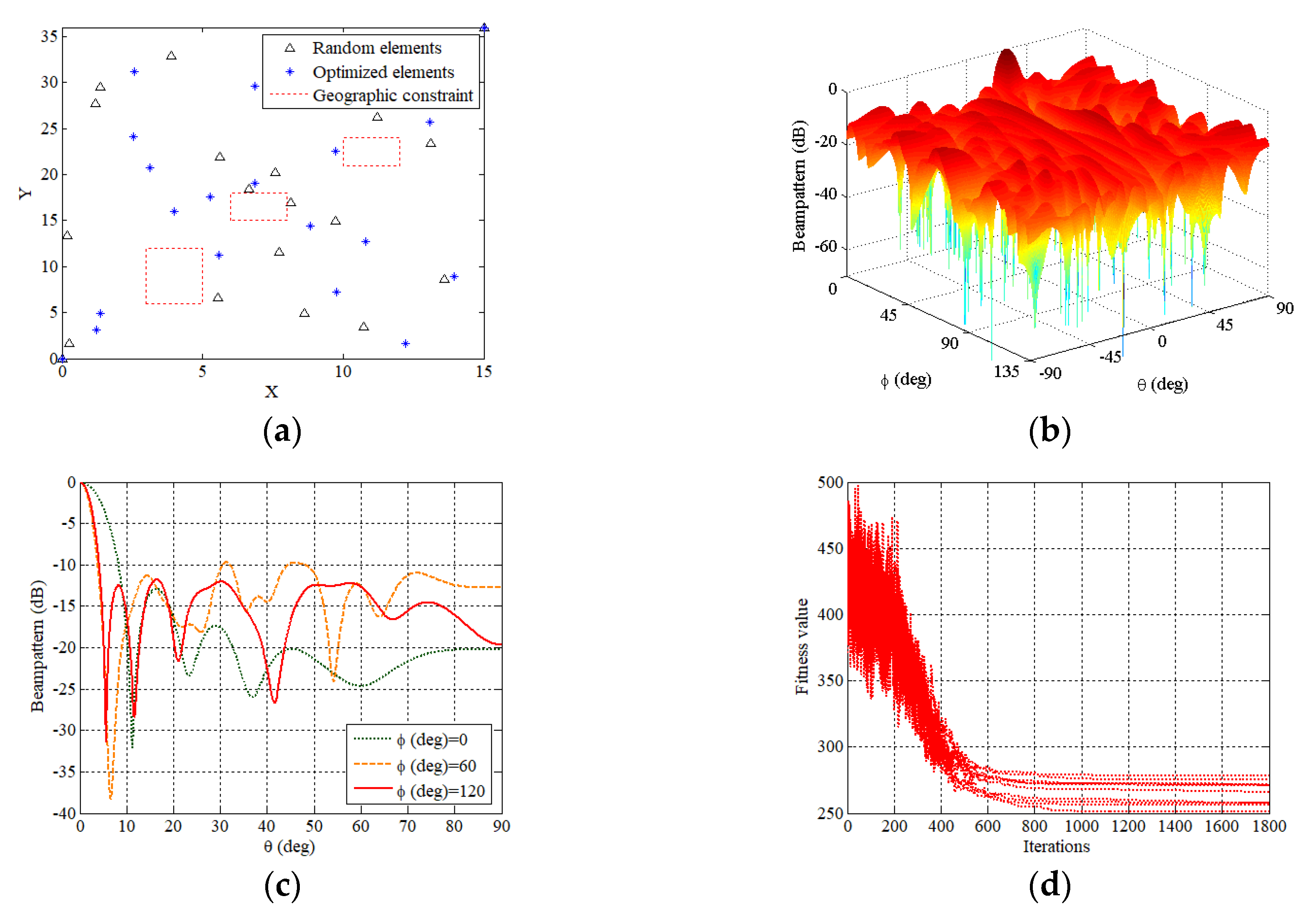
Assume that the SPA will be deployed in a geographic area of $D_X\times D_Y$, where $D_X=15$ and $D_Y=36$. The total number of elements $N=21$. The signal wavelength $\lambda$ is 3 and the minimum spacing constraint $\mathsf{\Delta }d=\lambda /2$. The total number of uniformly sampled elevation and azimuth scanning angles are both 7, i.e., $M=I=7$, the initial temperature $T$ is 100, and the iteration number $K$ in optimization is 1800. Three obstacles are considered, i.e., $x_n,y_n\notin \left(\left(3,5\right){{\displaystyle \cap }}^{\text{}}\left(6,12\right)\right){{\displaystyle \cup }}^{\text{}}\left(\left(6,8\right){{\displaystyle \cap }}^{\text{}}\left(15,18\right)\right){{\displaystyle \cup }}^{\text{}}\left(\left(10,12\right){{\displaystyle \cap }}^{\text{}}\left(21,24\right)\right),n=1,\cdots ,N-2$.

Two sparse planar arrays with random and optimized deployment are shown in Figure 1a. The elements of both sparse planar arrays are not located in areas corresponding to geographic constraints, and the minimum spacing between any two adjacent elements is greater than $\mathsf{\Delta }d$. The beampattern of the optimized sparse planar array when the peak of the main-lobe is at $\left(30°,0°\right)$ is given in Figure 1b. Figure 1c shows the beampatterns in $\phi =0°$, $\phi =60°$ and $\phi =120°$ planes whose PSLLs are −12.9 dB, −9.69 dB and −11.76 dB, respectively. It is shown the optimization of sparse planar arrays with minimum spacing and geographic constraints is successfully implemented in Figure 1a–c. The good convergences of the fitness value ($f$ in Equation (5)) versus the number of iterations through 10 trials are shown in Figure 1d.

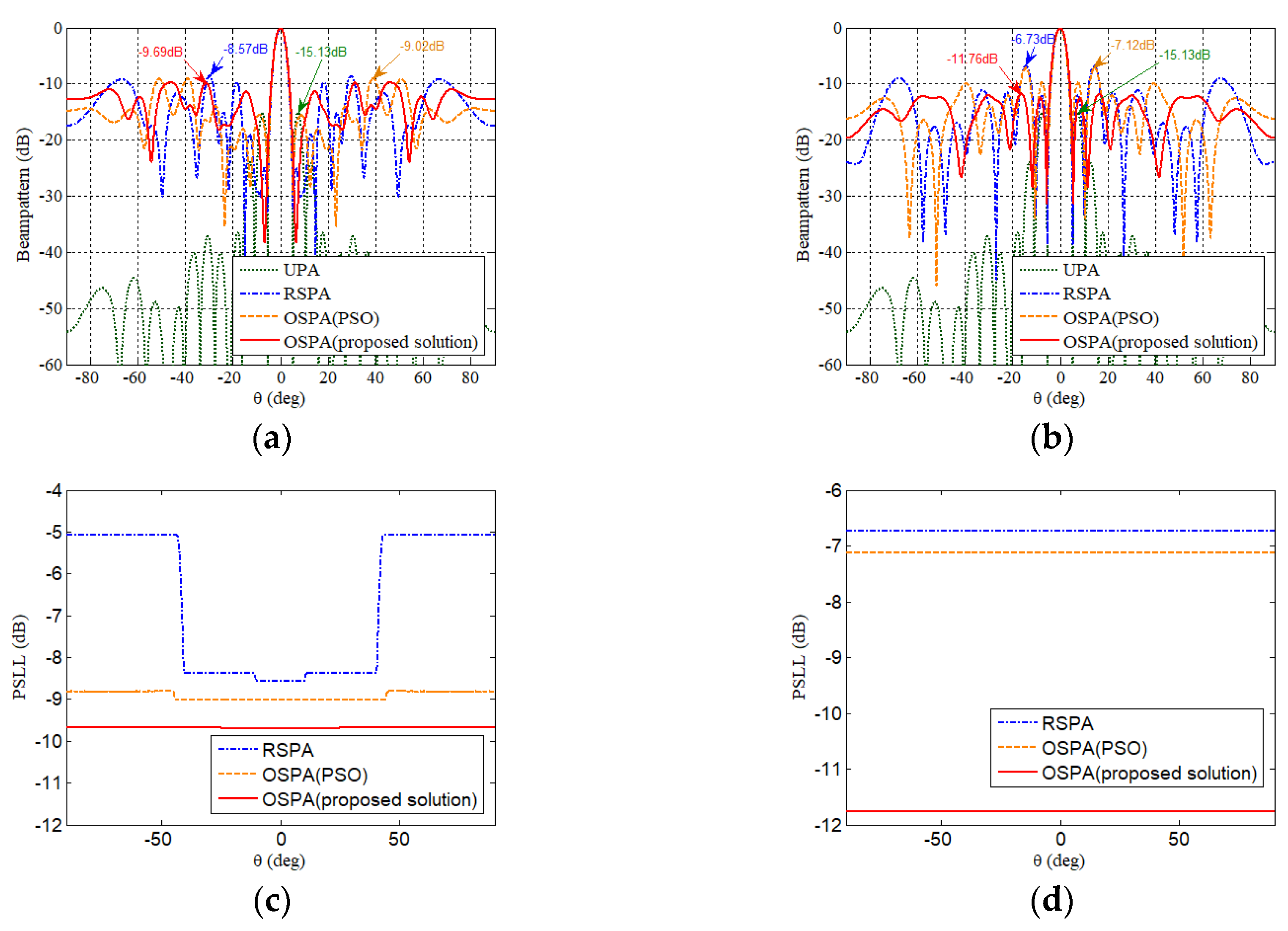
Figure 2a,b illustrate the beampatterns of the optimized sparse planar array (OSPA), respectively by the proposed solution and PSO [12,13,24], random sparse planar array (RSPA) without optimization, and uniform planar array (UPA) in $\phi =60°$ and $\phi =120°$ planes. The UPA has 275 elements and is also deployed in the same area. It is shown that their main-lobe beam widths are almost at the same level, which means that the spare planar array can have a larger array aperture with a smaller number of elements for high angular resolution. The PSLLs of beampatterns versus different beam shifting directions for the UPA, the RSPA, and the OSPA optimized by the proposed solution and PSO in $\phi =60°$ and $\phi =120°$ planes are illustrated in Figure 2c,d. In Figure 2, the side-lobe level of the OSPA is higher than that of the UPA but significantly lower than that of the RSPA. Generally, the low side-lobe level is very important for interference suppression in target localization.

5. Robustness of a Deployment-Optimized SPA

The optimization of a sparse planar array with minimum spacing and geographic constraints yields a distribution of elements optimized for high angular resolution and low side-lobe level, which means that the performance of the optimized sparse planar array in practical applications may be sensitive to mismatching, e.g., mis-calibration in hydrophone arrays or distributed underwater acoustic sensor networks, in which case the array deployment would have extremely strict accuracy requirements for the location of elements. Thus, the robustness of the deployment-optimized sparse planar array against mismatching is further considered in this paper.

Assume that the observation $\mathrm{X}\left(t\right)$ received by the sparse planar array in the presence of additive white Gaussian noise (AWGN) can be expressed by:

$$\mathrm{X}\left(t\right)=\mathrm{AS}\left(t\right)+\mathrm{N}\left(t\right),$$

(15)

where $\mathrm{A}$ is the steering matrix, and $\mathrm{S}\left(t\right)$ and $\mathrm{N}\left(t\right)$ correspond to the signals and noise, respectively.

The standard Capon beamformer (SCB) and robust Capon beamformer (RCB) are always taken together for performance comparison when the mismatching occurs. Generally, the RCB belongs to the class of diagonal loading techniques [37]. The SCB has the optimal weight ${\mathrm{w}}_0={\widehat{\mathrm{R}}}_{\mathrm{X}}^{-1}{\mathrm{a}}_0/{\mathrm{a}}_0^H{\widehat{\mathrm{R}}}_{\mathrm{X}}^{-1}{\mathrm{a}}_0$, and the weight vector of RCB is generally given by:

$${\mathrm{w}}_{\mathrm{DL}}=\frac{{\left({\widehat{\mathrm{R}}}_{\mathrm{X}}+\lambda I\right)}^{-1}{\mathrm{a}}_0}{{\mathrm{a}}_0^H{\left({\widehat{\mathrm{R}}}_{\mathrm{X}}+\lambda I\right)}^{-1}{\mathrm{a}}_0},$$

(16)

where ${\widehat{\mathrm{R}}}_{\mathrm{X}}$ is the covariance matrix estimate of $\mathrm{X}\left(t\right)$ and ${\widehat{\mathrm{R}}}_{\mathrm{X}}{{\displaystyle \sum }}_{t=1}^{N_t}\mathrm{X}\left(t\right){\mathrm{X}}^H\left(t\right)/N_t$, $N_t$ is the number of snapshots. $\lambda$ in Equation (16) is the diagonal loading value and can be often effectively determined as follows [38]:

$$\mathrm{std}\left(\mathrm{diag}\right({\widehat{\mathrm{R}}}_{\mathrm{X}}\left)\right)\le \lambda \le \mathrm{trace}\left({\widehat{\mathrm{R}}}_{\mathrm{X}}\right)/N$$

(17)

where $\mathrm{std}(·)$ means the standard deviation and $\mathrm{diag}(·)$ means the diagonal elements of a matrix. In this paper, we let $\lambda =\mathrm{std}\left(\mathrm{diag}\left({\widehat{\mathrm{R}}}_{\mathrm{X}}\right)\right)$.

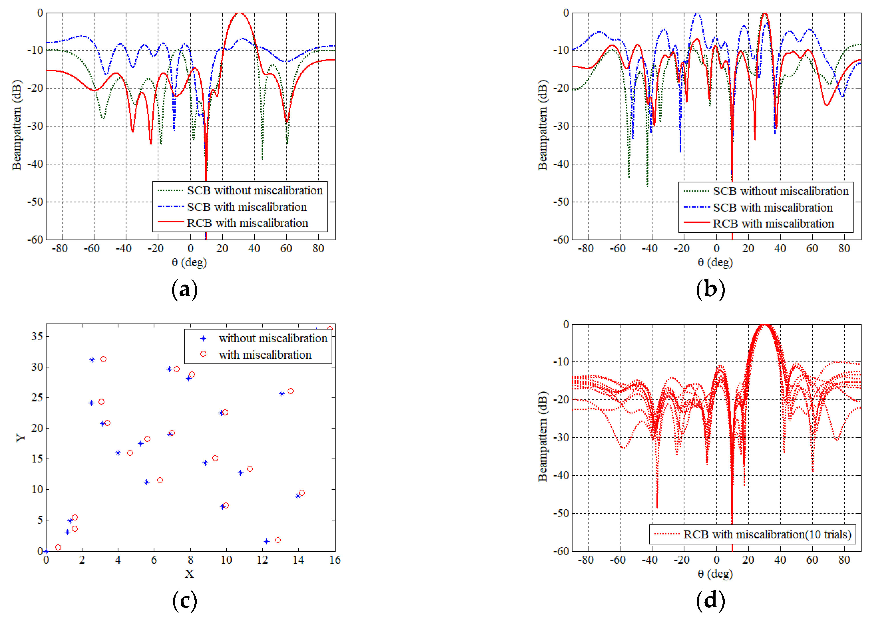
The performance comparison is given in Figure 3a,b, where standard Capon beamforming (SCB) without mis-calibration, SCB with mis-calibration, and robust Capon beamforming (RCB) with mis-calibration are presented. The mis-calibration in simulations is assumed to have a Gaussian distribution with a standard deviation of Δd/2. The elements are illustrated in Figure 3c. It is shown the OSPA with miscalibration still has good performance by taking the robust adaptive beamforming. Figure 3d shows the beampatterns of RCB with mis-calibration through 10 trials.

6. Conclusions

In this paper, the optimization of SPAs in smart ocean applications with minimum spacing and geographic constraints has been presented, where the cost function is defined as the sum of PSLL for different beam shifting directions and simulated annealing has been used for the optimization. The implementation of these constraints in optimization is also given. Furthermore, the robustness of the deployment-optimized SPA against mis-calibration of the array in practical applications is also verified. Simulations show that the optimized SPA is effective for the DOA estimation.

References

- Song, H.; Cho, S.; Kang, T.; Hodgkiss, W.; Preston, J. Long-range acoustic communication in deep water using a towed array. J. Acoust. Soc. Am. 2011, 129, 71–75. [Google Scholar] [CrossRef] [PubMed]
- Makris, N.C.; Ratilal, P.; Symonds, D.T.; Jagannathan, S.; Lee, S.; Nero, R.W. Fish population and behavior revealed by instantaneous continental shelf-scale imaging. Science 2006, 311, 660–663. [Google Scholar] [CrossRef]
- Huang, W.; Wang, D.; Garcia, H.; Godø, O.R.; Ratilal, P. Continental shelf-scale passive acoustic detection and characterization of diesel-electric ships using a coherent hydrophone array. Remote Sens. 2017, 9, 772. [Google Scholar] [CrossRef]
- Zhu, C.; Garcia, H.; Kaplan, A.; Schinault, M.; Handegard, N.; Godø, O.; Huang, W.; Ratilal, P. Detection, localization and classification of multiple mechanized ocean vessels over continental-shelf scale regions with passive ocean acoustic waveguide remote sensing. Remote Sens. 2018, 10, 1699. [Google Scholar] [CrossRef]
- Wang, D.; Ratilal, P. Angular resolution enhancement provided by nonuniformly-spaced linear hydrophone arrays in ocean acoustic waveguide remote sensing. Remote Sens. 2017, 9, 1036. [Google Scholar] [CrossRef]
- Trucco, A.; Martelli, S.; Crocco, M. Passive underwater imaging through optimized planar arrays of hydrophones. In Proceedings of the 2014 Oceans-St. John’s Conference, St. John’s, NL, Canada, 14–19 September 2014. [Google Scholar]
- Han, G.; Qian, A.; Zhang, C.; Wang, Y.; Rodrigues, J.J. Localization algorithms in large-scale underwater acoustic sensor networks: A quantitative comparison. Int. J. Distrib. Sens. Netw. 2014, 10, 379382. [Google Scholar] [CrossRef]
- Han, G.; Jiang, J.; Shu, L.; Xu, Y.; Wang, F. Localization algorithms of underwater wireless sensor networks: A survey. Sensors 2012, 12, 2026–2061. [Google Scholar] [CrossRef]
- Han, G.; Li, S.; Zhu, C.; Jiang, J.; Zhang, W. Probabilistic neighborhood-based data collection algorithms for 3D underwater acoustic sensor networks. Sensors 2017, 17, 316. [Google Scholar] [CrossRef]
- Busby, D. Hierarchical adaptive experimental design for Gaussian process emulators. Reliab. Eng. Syst. Saf. 2009, 94, 1183–1193. [Google Scholar] [CrossRef]
- Martino, L.; Vicent, J.; Camps-Valls, G. Automatic emulator and optimized look-up table generation for radiative transfer models. In Proceedings of the 2017 IEEE International Geoscience and Remote Sensing Symposium (IGARSS), Fort Worth, TX, USA, 23–28 July 2017. [Google Scholar]
- Khodier, M.M.; Christodoulou, C.G. Linear array geometry synthesis with minimum sidelobe level and null control using particle swarm optimization. IEEE Trans. Antennas Propag. 2005, 53, 2674–2679. [Google Scholar] [CrossRef]
- Bhattacharya, R.; Bhattacharyya, T.K.; Garg, R. Position mutated hierarchical particle swarm optimization and its application in synthesis of unequally spaced antenna arrays. IEEE Trans. Antennas Propag. 2012, 60, 3174–3181. [Google Scholar] [CrossRef]
- Haupt, R.L. Thinned arrays using genetic algorithms. IEEE Trans. Antennas Propag. 1994, 42, 993–999. [Google Scholar] [CrossRef]
- Yan, K.K.; Lu, Y. Sidelobe reduction in array-pattern synthesis using genetic algorithm. IEEE Trans. Antennas Propag. 1997, 45, 1117–1122. [Google Scholar]
- Cen, L.; Ser, W.; Yu, Z.L.; Rahardja, S. An improved genetic algorithm for aperiodic array synthesis. In Proceedings of the 2008 IEEE International Conference on Acoustics, Speech and Signal Processing, Las Vegas, NV, USA, 31 March–4 April 2008; pp. 2465–2468. [Google Scholar]
- Trucco, A.; Murino, V. Stochastic optimization of linear sparse arrays. IEEE J. Ocean. Eng. 1999, 24, 291–299. [Google Scholar] [CrossRef]
- Lin, J.C.; Ma, X.C.; Yan, S.F.; Jiang, L. Pattern synthesis of sparse linear array by off-grid Bayesian compressive sampling. Electron. Lett. 2015, 51, 2141–2143. [Google Scholar] [CrossRef]
- Schumer, M.A.; Steiglitz, K. Adaptive step size random search. IEEE Trans. Autom. Control 1968, 13, 270–276. [Google Scholar] [CrossRef] [Green Version]
- Martino, L.; Elvira, V.; Luengo, D.; Corander, J.; Louzada, F. Orthogonal parallel MCMC methods for sampling and optimization. Digit. Signal Process. 2016, 58, 64–84. [Google Scholar] [CrossRef] [Green Version]
- Geyer, C.J. Markov Chain Monte Carlo Maximum Likelihood; Interface Foundation of North America: Fairfax Station, VA, USA, 1991. [Google Scholar]
- Hawes, M.B.; Liu, W. Location optimization of robust sparse antenna arrays with physical size constraint. IEEE Antennas Wirel. Propag. Lett. 2012, 11, 1303–1306. [Google Scholar] [CrossRef]
- Hawes, M.B.; Liu, W. Compressive sensing-based approach to the design of linear robust sparse antenna arrays with physical size constraint. IET Microw. Antennas Propag. 2014, 8, 736–746. [Google Scholar] [CrossRef] [Green Version]
- Yu, X.; Cui, G.; Yang, S.; Kong, L.; Yi, W. Coherent unambiguous transmit for sparse linear array with geography constraint. IET Radar Sonar Navig. 2017, 11, 386–393. [Google Scholar] [CrossRef]
- Yan, C.; Yang, P.; Xing, Z.; Huang, S.Y. Synthesis of planar sparse arrays with minimum spacing constraint. IEEE Antennas Wirel. Propag. Lett. 2018, 17, 1095–1098. [Google Scholar] [CrossRef]
- Pinchera, D.; Migliore, M.D.; Panariello, G. Synthesis of large sparse arrays using IDEA (inflating-deflating exploration algorithm). IEEE Trans. Antennas Propag. 2018, 66, 4658–4668. [Google Scholar] [CrossRef]
- Chen, K.S.; Yun, X.H.; He, Z.S. Synthesis of sparse planar arrays using modified real genetic algorithm. IEEE Trans. Antennas Propag. 2007, 55, 1067–1073. [Google Scholar] [CrossRef]
- Liu, H.; Zhao, H.; Li, W.; Liu, B. Synthesis of sparse planar arrays using matrix mapping and differential evolution. IEEE Antennas Wirel. Propag. Lett. 2016, 15, 1905–1908. [Google Scholar] [CrossRef]
- Dai, D.; Yao, M.; Ma, H.; Jin, W.; Zhang, F. An asymmetric mapping method for the synthesis of sparse planar arrays. IEEE Antennas Wirel. Propag. Lett. 2018, 17, 70–73. [Google Scholar] [CrossRef]
- Impagliazzo, J.M.; Kay, S.M.; Chiang, A.M.; Broadstone, S.R. Sparse array technology for 3-D sonar imaging systems. J. Acoust. Soc. Am. 1999, 106, 2296–2297. [Google Scholar] [CrossRef]
- Wong, K.T.; Zoltowski, M.D. Direction-finding with sparse rectangular dual-size spatial invariance array. IEEE Trans. Aerosp. Electron. Syst. 1998, 34, 1320–1336. [Google Scholar] [CrossRef]
- Cheng, Z.F.; Zhao, Y.B.; Li, H.; Shui, P.L. Two-dimensional DOA estimation algorithm with co-prime array via sparse representation. Electron. Lett. 2015, 51, 2084–2086. [Google Scholar] [CrossRef]
- Long, T.; Zhang, H.; Zeng, T.; Chen, X.; Liu, Q.; Zheng, L. Target tracking using SePDAF under ambiguous angles for distributed array radar. Sensors 2016, 16, 1456. [Google Scholar] [CrossRef] [PubMed]
- Mailloux, R.J. Phased Array Antenna Handbook; Artech House: Norwood, MA, USA, 2017; pp. 12–17. [Google Scholar]
- Salomon, K.B. An efficient point-in-polygon algorithm. Comput. Geosci. 1978, 4, 173–178. [Google Scholar] [CrossRef]
- Kirkpatrick, S.; Gellatt, C.D., Jr.; Vecchi, M.P. Optimization by simulated annealing. Science 1983, 220, 671–680. [Google Scholar] [CrossRef] [PubMed]
- Li, J.; Stoica, P. Robust Adaptive Beamforming; John Wiley & Sons: Hoboken, NJ, USA, 2005. [Google Scholar]
- Ma, N.; Goh, J.T. Efficient method to determine diagonal loading value. In Proceedings of the 2003 IEEE International Conference on Acoustics, Speech, and Signal Processing, Hong Kong, China, 6–10 April 2003. [Google Scholar]
Figure 1.
(a) The 21-element sparse planar arrays with random and optimized deployment that satisfy the minimum spacing and geographic constraints. (b) The beampattern of the optimized sparse planar array when the peak of the main-lobe is at . (c) The beampatterns in , , and planes. (d) The convergences of the fitness value versus the number of iterations through 10 trials.
Figure 2.
The beampatterns of the RSPA, the UPA and the OSPA by the proposed solution and PSO in (a) the plane (the main-lobe is at ) and (b) the plane (the main-lobe is at ). The PSLLs of beampatterns versus different beam shifting directions in the (c) , and (d) planes.
Figure 3.
Comparison of the beampatterns in the (a) and (b) plane of the SCB without mis-calibration, the SCB and the RCB with mis-calibration. (c) The elements’ locations with and without mis-calibration. (d) The beampatterns of RCB with mis-calibration through 10 trials.
© 2018 by the authors. Licensee MDPI, Basel, Switzerland. This article is an open access article distributed under the terms and conditions of the Creative Commons Attribution (CC BY) license (http://creativecommons.org/licenses/by/4.0/).
Share and Cite
MDPI and ACS Style
Hao, S.; Ge, F.-X.; Yu, X.; Cui, G.; Ma, L. Optimization of Sparse Planar Arrays with Minimum Spacing and Geographic Constraints in Smart Ocean Applications. Sensors 2019, 19, 11. https://doi.org/10.3390/s19010011
AMA Style
Hao S, Ge F-X, Yu X, Cui G, Ma L. Optimization of Sparse Planar Arrays with Minimum Spacing and Geographic Constraints in Smart Ocean Applications. Sensors. 2019; 19(1):11. https://doi.org/10.3390/s19010011
Chicago/Turabian StyleHao, Shijie, Feng-Xiang Ge, Xianxiang Yu, Guolong Cui, and Li Ma. 2019. "Optimization of Sparse Planar Arrays with Minimum Spacing and Geographic Constraints in Smart Ocean Applications" Sensors 19, no. 1: 11. https://doi.org/10.3390/s19010011
Note that from the first issue of 2016, this journal uses article numbers instead of page numbers. See further details here.