Convolutional Neural Networks Approach for Solar Reconstruction in SCAO Configurations

 , , and
Abstract
:1. Introduction
2. Materials and Methods
2.1. Adaptive Optics
2.2. Adaptive Optics for Solar Observations
2.3. Artificial Neural Networks
- Input set .
- Synaptic weights ; indicate the intensity of interaction with the neuron the weight that the received/given information will have.
- Activation function corresponds to the final output of the neuron; including the bias.
2.4. Simulation Setup
2.4.1. Several Solar frames.
- Simulations.During the simulations, several offsets were established to select the different frames of the solar image; eight values for pixels in the coordinates and 10 values for the pixels on the ordinates, giving a result of 80 different combinations. These conformed the regions of the sun to be trained with.The simulated SH had 10 subapertures per side, with a resolution of 28 pixels of side per subaperture. The simulated outputs corresponded with the 117 active DM actuators.For the training set, a fixed value of 0.12 cm for the , taking as example the performance of other ANNs in nocturnal AO when trained [54,55]. The height steps of the turbulence were 1 km each, from 0 to 15 km of altitude. Each combination of all the above information was repeated for 100 iterations each, giving a total of 128,000 training samples.
- Network.The topology of the network was selected after a grid search on its hyperparameters; considering different number and sizes of kernels, as well as number of neurons on the hidden layer. Only one hidden layer was used to minimize the vanishing gradient influence. In particular, the topology consisted on four convolutional layers, with 8, 2, 2 and 2 kernels, respectively. The size of those kernels was of 5 × 5 pixels, with stride steps of 1 in both directions; additionally, padding was added. All the convolutional layers used Leaky-ReLU as activation function and were followed by max-pooling of 2 × 2 pixels for the first three layers and 5 × 5 pixels for the last one. As the image from each sample was square of 280 pixels of side, the resulting 64 images of 7 pixels of side were reshaped to a vector of 3136 components to be used as inputs of the MLP section of the network. A hidden layer was set with 1024 neurons, with Leaky-ReLU as activation function. The output layer is set for 117 neurons, corresponding with the actuator values, without any activation function. The network was trained with Adagrad procedure, using MSE as loss function, with learning rate of 0.001 and momentum of 0.9.
2.4.2. Fixed Section of the Image
- Simulations.The sizes from both the SH and the DM remains the same as the previous case, with 10 subapertures per side of the simulated SH, with resolution of 28 pixels of side per subaperture, and 117 active DM actuators.The training set had a fixed value of 0.12 cm for the , and height steps of 10 meters each, from 0 to 15 km of altitude. Each step was repeated for 100 iterations each, giving a total of 150,000 training samples. For establishing the test set, two approaches were taken.
- (1)
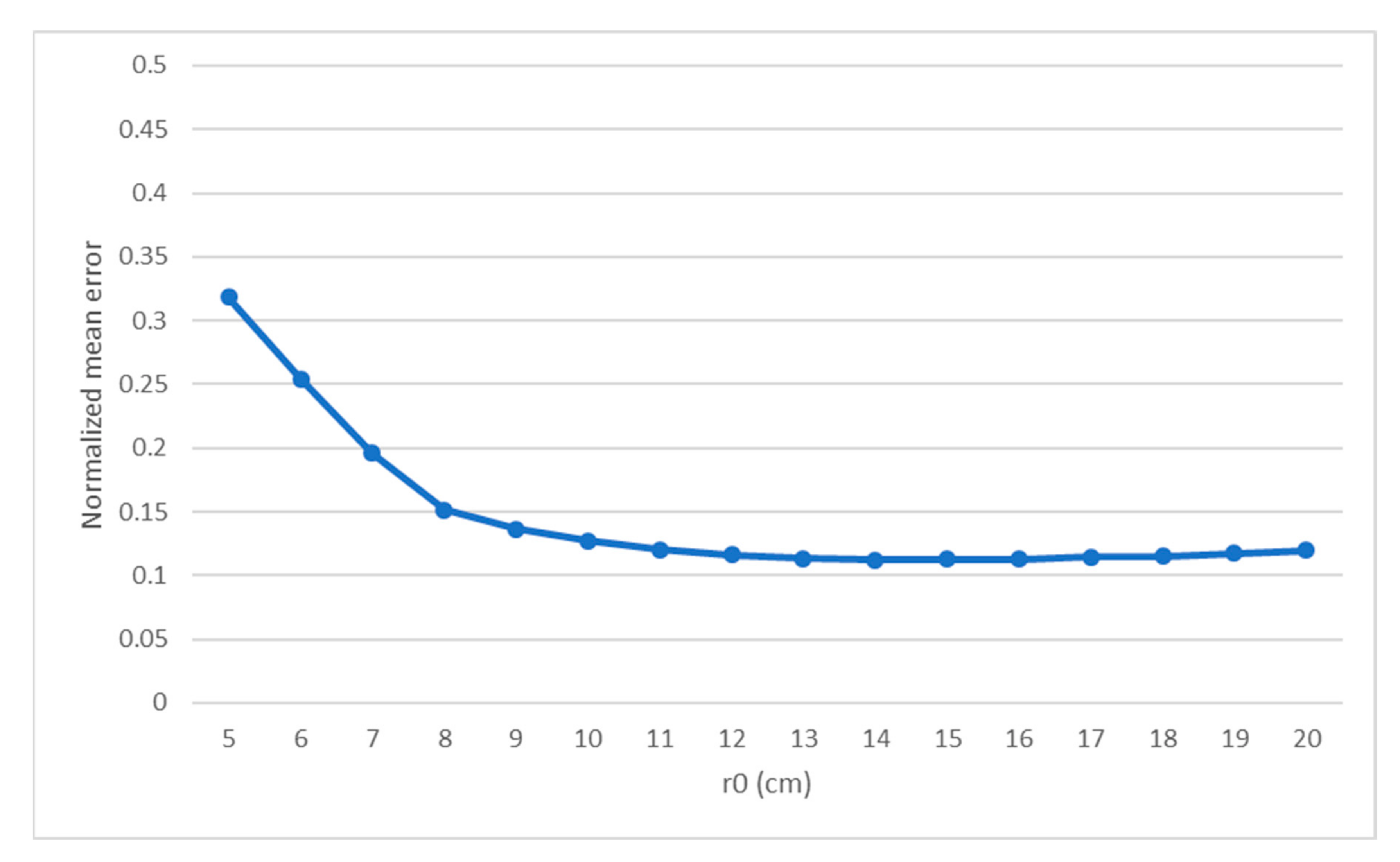
- Fixed tests. The test set were simulated for a fixed with height steps ok 1 km each. Varying the from 5 to 20 cm conformed the 16 tests set used.
- (2)
- Network.As in the previous case, the topology of the network was set after a grid search on its hyperparameters, considering kernel number, size, number of hidden layer neurons, etc., selecting those that increased the performance of the model. The reconstructor proto-HELIOS consists of a convolutional neural network with four convolutional layers, each one with two kernels of 5 × 5 pixels each. All the layers use Leaky-ReLU as activation function, with strides of 1 for the kernels and adding padding in every convolutional layer, all the layers are followed by max-pooling of 2 × 2 pixels in the first 2 layers, with a 5 × 5 pixel pooling for the third one and a 7 × 7 pixel pooling for the last one.The convolutions result in 16 images of 2 × 2 pixels, which are reshaped in a vector to be used as the inputs of the MLP section of the network. The hidden layer has 1024 neurons, and the output has 117 neurons. Both the hidden and the output layer have Leaky-ReLU as activation function.The network was trained with Adagrad procedure, using MSE as loss function, with learning rate of 0.001 and momentum of 0.9.
3. Results
3.1. Several Solar Frames
3.2. Fixed Section of the Image
4. Discussion
5. Conclusions
Author Contributions
Funding
Conflicts of Interest
References
- Roddier, F. Adaptive Optics in Astronomy; Cambridge University Press: Cambridge, UK, 1999. [Google Scholar]
- Beckers, J.M. Adaptive optics for astronomy: Principles, performance, and applications. Annu. Rev. Astron. Astrophys. 1993, 31, 13–62. [Google Scholar] [CrossRef]
- Montilla, I.; Marino, J.; Ramos, A.A.; Collados, M.; Montoya, L.; Tallon, M. Solar adaptive optics: Specificities, lessons learned, and open alternatives. In Proceedings of the SPIE Astronomical Telescopes + Instrumentation, Edigburgh, Scotland, 26 June–1 July 2016; p. 99091H. [Google Scholar]
- Platt, B.C.; Shack, R. History and principles of Shack-Hartmann wavefront sensing. J. Refract. Surg. 2001, 17, S573–S577. [Google Scholar] [CrossRef]
- Roddier, F. Curvature sensing and compensation: A new concept in adaptive optics. Appl. Opt. 1988, 27, 1223. [Google Scholar] [CrossRef]
- Wu, C.; Ko, J.; Davis, C.C. Determining the phase and amplitude distortion of a wavefront using a plenoptic sensor. J. Opt. Soc. Am. A 2015, 32, 964. [Google Scholar] [CrossRef]
- Iglesias, I.; Ragazzoni, R.; Julien, Y.; Artal, P. Extended source pyramid wave-front sensor for the human eye. Opt. Express 2002, 10, 419. [Google Scholar] [CrossRef] [PubMed]
- Rimmele, T.R.; Radick, R.R. Solar adaptive optics at the national solar observatory. In Adaptive Optical System Technologies; Bonaccini, D., Tyson, R.K., Eds.; 1998; Volume 3353, pp. 72–82. [Google Scholar]
- Sidick, E.; Green, J.J.; Morgan, R.M.; Ohara, C.M.; Redding, D.C. Adaptive cross-correlation algorithm for extended scene Shack-Hartmann wavefront sensing. Opt. Lett. 2008, 33, 213–215. [Google Scholar] [CrossRef] [PubMed]
- Brown, L.G. A survey of image registration techniques. ACM Comput. Surv. 1992, 24, 325–376. [Google Scholar] [CrossRef]
- Collados, M.; Bettonvil, F.; Cavaller, L.; Ermolli, I.; Gelly, B.; Pérez, A.; Socas-Navarro, H.; Soltau, D.; Volkmer, R. European solar telescope: Progress status. Astron. Nachr. 2010, 331, 609–614. [Google Scholar] [CrossRef]
- Scharmer, G.B.; Bjelksjo, K.; Korhonen, T.K.; Lindberg, B.; Petterson, B. The 1-meter Swedish solar telescope. In Innovative Telescopes and Instrumentation for Solar Astrophysics; Keil, S.L., Avakyan, S.V., Eds.; Society of Photo Optical: Bellingham, WA, USA, 2003; Volume 4853, pp. 341–351. [Google Scholar]
- Scharmer, G.B.; Dettori, P.M.; Lofdahl, M.G.; Shand, M. Adaptive optics system for the new Swedish solar telescope. In Innovative Telescopes and Instrumentation for Solar Astrophysics; Keil, S.L., Avakyan, S.V., Eds.; Society of Photo Optical: Bellingham, WA, USA, 2003; Volume 4853, pp. 370–381. [Google Scholar]
- Dalimier, E.; Dainty, C. Comparative analysis of deformable mirrors for ocular adaptive optics. Opt. Express 2005, 13, 4275. [Google Scholar] [CrossRef] [PubMed]
- Matthews, S.A.; Collados, M.; Mathioudakis, M.; Erdelyi, R. The European solar telescope (EST). In Ground Based Airborne Instrum. Astron. VI; Evans, C.J., Simard, L., Takami, H., Eds.; Society of Photo Optical: Bellingham, WA, USA, 2016; Volume 9908, p. 990809. [Google Scholar]
- Berkefeld, T.; Bettonvil, F.; Collados, M.; López, R.; Martin, Y.; Peñate, J.; Pérez, A.; Scharmer, G.B.; Sliepen, G.; Soltau, D.; et al. Site-seeing measurements for the European solar telescope. In Ground-based and Airborne Telescopes III; Stepp, L.M., Gilmozzi, R., Hall, H.J., Eds.; Society of Photo Optical: Bellingham, WA, USA, 2010; Volume 7733, p. 77334I. [Google Scholar]
- Dwivedi, A.K. Artificial neural network model for effective cancer classification using microarray gene expression data. Neural Comput. Appl. 2016, 29, 1–10. [Google Scholar] [CrossRef]
- Lasheras, J.E.S.; Donquiles, C.G.; Nieto, P.J.G.; Moleon, J.J.J.; Salas, D.; Gómez, S.L.S.; de la Torre, A.J.M.; González-Nuevo, J.; Bonavera, L.; Landeira, J.C.; et al. A methodology for detecting relevant single nucleotide polymorphism in prostate cancer with multivariate adaptive regression splines and backpropagation artificial neural networks. Neural Comput. Appl. 2018, 1–8. [Google Scholar] [CrossRef]
- Krizhevsky, A.; Sutskever, I.; Hinton, G.E. Imagenet classification with deep convolutional neural networks. Adv. Neur. Inf. Proc. Syst. 2012, 1097–1105. [Google Scholar]
- LeCun, Y.; Bengio, Y.; Hinton, G. Deep learning. Nature 2015, 521, 436–444. [Google Scholar] [CrossRef]
- Suárez Gómez, S.L.; Santos Rodríguez, J.D.; Iglesias Rodríguez, F.J.; de Cos Juez, F.J. Analysis of the temporal structure evolution of physical systems with the self-organising tree algorithm (SOTA): Application for validating neural network systems on adaptive optics data before on-sky implementation. Entropy 2017, 19, 103. [Google Scholar] [CrossRef]
- Osborn, J.; Juez, F.J.D.C.; Guzman, D.; Butterley, T.; Myers, R.; Guesalaga, A.; Laine, J.; de Cos Juez, F.J.; Guzman, D.; Butterley, T.; et al. Using artificial neural networks for open-loop tomography. Opt. Express 2012, 20, 2420–2434. [Google Scholar] [CrossRef]
- Ellerbroek, B.L. First-order performance evaluation of adaptive-optics systems for atmospheric-turbulence compensation in extended-field-of-view astronomical telescopes. JOSA A 1994, 11, 783–805. [Google Scholar] [CrossRef]
- Hampton, P.J.; Agathoklis, P.; Bradley, C. A new wave-front reconstruction method for adaptive optics systems using wavelets. IEEE J. Sel. Top. Sig. Process. 2008, 2, 781–792. [Google Scholar] [CrossRef]
- Dai, G. Modal wave-front reconstruction with Zernike polynomials and Karhunen–Loève functions. J. Opt. Soc. Am. A 2008, 13, 1218. [Google Scholar] [CrossRef]
- Zilberman, A.; Golbraikh, E.; Kopeika, N.S. Propagation of electromagnetic waves in Kolmogorov and non-Kolmogorov atmospheric turbulence: Three-layer altitude model. Appl. Opt. 2008, 47, 6385–6391. [Google Scholar] [CrossRef]
- Fried, D.L. Optical resolution through a randomly inhomogeneous medium for very long and very short exposures. JOSA 1966, 56, 1372–1379. [Google Scholar] [CrossRef]
- Greenwood, D.P. Bandwidth specification for adaptive optics systems. JOSA 1977, 67, 390–393. [Google Scholar] [CrossRef]
- Tyson, R. Principles of Adaptive Optics; CRC Press: Boca Raton, FL, USA, 2010. [Google Scholar]
- Freeman, R.H.; Pearson, J.E. Deformable mirrors for all seasons and reasons. Appl. Opt. 1982, 21, 580–588. [Google Scholar] [CrossRef] [PubMed]
- Basden, A.G.; Atkinson, D.; Bharmal, N.A.; Bitenc, U.; Brangier, M.; Buey, T.; Butterley, T.; Cano, D.; Chemla, F.; Clark, P.; et al. Experience with wavefront sensor and deformable mirror interfaces for wide-field adaptive optics systems. Mon. Not. R. Astron. Soc. 2016, 459, 1350–1359. [Google Scholar] [CrossRef]
- Gendron, E.; Vidal, F.; Brangier, M.; Morris, T.; Hubert, Z.; Basden, A.; Rousset, G.; Myers, R.; Chemla, F.; Longmore, A.; et al. MOAO first on-sky demonstration with CANARY. Astron. Astrophys. 2011, 529, L2. [Google Scholar] [CrossRef]
- Juez, F.J.; Lasheras, F.S.; Roqueñi, N.; Osborn, J.; de Cos Juez, F.J.; Lasheras, F.S.; Roqueñí, N.; Osborn, J.; Juez, F.J.; Lasheras, F.S.; et al. An ANN-based smart tomographic reconstructor in a dynamic environment. Sensors 2012, 12, 8895–8911. [Google Scholar] [CrossRef] [PubMed]
- Davies, R.; Kasper, M. Adaptive optics for astronomy. Annu. Rev. Astron. Astrophys. 2012, 50, 305–351. [Google Scholar] [CrossRef]
- Rimmele, T.R. Recent advances in solar adaptive optics. In Advancements in Adaptive Optics; Bonaccini Calia, D., Ellerbroek, B.L., Ragazzoni, R., Eds.; Society of Photo Optical: Bellingham, WA, USA, 2004; Volume 5490, pp. 34–47. [Google Scholar]
- Berkefeld, T.; Soltau, D.; Mats, L. Wavefront Sensing and Wavefront Reconstruction for the 4m European Solar Telescope EST. Int. Soc. Opt. Photon. 2010, 7736, 1–9. [Google Scholar]
- Berkefeld, T. Solar adaptive optics. In Modern Solar Facilities-Advanced Solar Science; Franz, K., Klaus, G.P., Wittmann, A.D., Eds.; Universitätsverlag Göttingen: Göttingen, Germany, 2007; p. 107. [Google Scholar]
- Rimmele, T.; Dunn, R.; Richards, K.; Radick, R. Solar adaptive optics at the National Solar Observatory. In High Resolution Solar Physics: Theory, Observations, and Techniques; Rimmele, T.R., Balasubramaniam, K.S., Radick, R.R., Eds.; Astronomical Society of the Pacific: San Francisco, CA, USA, 1999; Volume 183, p. 222. [Google Scholar]
- Von Der Lühe, O.; Widener, A.L.; Rimmele, T.; Spence, G.; Dunn, R.B. Solar feature correlation tracker for ground-based telescopes. Astron. Astrophys. 1989, 224, 351–360. [Google Scholar]
- Knutsson, P.A.; Owner-Petersen, M.; Dainty, C. Extended object wavefront sensing based on the correlation spectrum phase. Opt. Express 2005, 13, 9527–9536. [Google Scholar] [CrossRef] [PubMed]
- Bracewell, R.N.; Bracewell, R.N. The Fourier Transform and Its Applications; McGraw-Hill: New York, NY, USA, 1986; Volume 31999. [Google Scholar]
- Noll, R.J. Zernike polynomials and atmospheric turbulence. JOSA 1976, 66, 207–211. [Google Scholar] [CrossRef]
- Russell, S.J.; Norvig, P. Artificial Intelligence: A Modern Approach; Pearson Education Limited: Kuala Lumpur, Malaysia, 2016. [Google Scholar]
- Suárez Gómez, S.L.; González-gutiérrez, C.; Alonso, E.D.; Santos Rodríguez, J.D.; Sánchez Rodríguez, M.L.; Landeira, J.C.; Basden, A.; Osborn, J. Improving Adaptive Optics Reconstructions with a Deep Learning Approach; Springer International Publishing: New York, NY, USA, 2018; pp. 74–83. [Google Scholar]
- Horn, R.A. The hadamard product. Proc. Symp. Appl. Math. 1990, 40, 87–169. [Google Scholar]
- Suárez Gómez, S.L.; González-gutiérrez, C.; Alonso, E.D.; Santos Rodríguez, J.D.; Bonavera, L.; Fernández Valdivia, J.L.; Rodríguez, J.M.; Rodríguez Ramos, L.F. Compensating atmospheric turbulence with convolutional neural networks for defocused pupil image wave- front sensors. In Proceedings of the International Conference on Hybrid Artificial Intelligence Systems, Oviedo, Spain, 20–22 June 2018. [Google Scholar]
- Nair, V.; Hinton, G.E. Rectified linear units improve restricted boltzmann machines. In Proceedings of the 27th International Conference on Machine Learning, Haifa, Israel, 21–24 June 2010; pp. 807–814. [Google Scholar]
- Giusti, A.; Ciresan, D.C.; Masci, J.; Gambardella, L.M.; Schmidhuber, J. Fast image scanning with deep max-pooling convolutional neural networks. In Proceedings of the Image Processing (ICIP), 2013 20th IEEE International Conference on, Melbourne, Australia, 15–18 September 2013; pp. 4034–4038. [Google Scholar]
- Nielsen, M.A. Neural Networks and Deep Learning (2015). Available online: http//neuralnetworksanddeeplearning.com (accessed on 13 May 2019).
- Lecun, Y.; Bottou, L.; Bengio, Y.; Haffner, P. Gradient-based learning applied to document recognition. Proc. IEEE 1998, 86, 2278–2323. [Google Scholar] [CrossRef]
- Ruder, S. An overview of gradient descent optimization algorithms. arXiv Prepr. 2016, arXiv:1609.04747. [Google Scholar]
- Basden, A. DASP the Durham Adaptive optics Simulation Platform: Modelling and simulation of adaptive optics systems. Available online: https://github.com/agb32/dasp (accessed on 13 May 2019).
- Abadi, M.; Barham, P.; Chen, J.; Chen, Z.; Davis, A.; Dean, J.; Devin, M.; Ghemawat, S.; Irving, G.; Isard, M.; et al. Tensor flow: A system for large-scale machine learning. In Proceedings of the 12th USENIX Symposium on Operating Systems Design and Implementation, Savannah, GA, USA, 2–4 November 2016; Volume 16, pp. 265–283. [Google Scholar]
- Osborn, J.; Guzmán, D.; de Cos Juez, F.J.; Basden, A.G.; Morris, T.J.; Gendron, É.; Butterley, T.; Myers, R.M.; Guesalaga, A.; Lasheras, F.S.; et al. First on-sky results of a neural network based tomographic reconstructor: Carmen on Canary. In Adaptive Optics Systems IV; Marchetti, E., Close, L.M., Véran, J.-P., Eds.; International Society for Optics and Photonics: Bellingham, WA, USA, 2014; Volume 9148, p. 91484M. [Google Scholar]
- Suárez Gómez, S.L.; Gutiérrez, C.G.; Rodríguez, J.D.S.; Rodríguez, M.L.S.; Lasheras, F.S.; de Cos Juez, F.J. Analysing the performance of a tomographic reconstructor with different neural networks frameworks. In Proceedings of the International Conference on Intelligent Systems Design and Applications, Porto, Portugal, 14–16 December 2016; pp. 1051–1060. [Google Scholar]
- Suárez-Gómez, S.L.; González-Gutiérrez, C.; Sánchez-Lasheras, F.; Basden, A.G.; Montilla, I.; de Cos Juez, F.J.; Collados-Vera, M. An approach using deep learning for tomographic reconstruction in solar observation. In Proceedings of the Adaptive Optics for Extremely Large Telescopes 5, Instituto de Astrofísica de Canarias (IAC), Tenerife, Spain, 25–30 June 2017. [Google Scholar]


| Test | 1 | 2 | 3 |
|---|---|---|---|
| (m) | 0.085 | 0.16 | 0.12 |
| Turbulence heights (m) | [0, 6500, 10,000, 15,500] | [0, 4000, 10,000, 15,500] | [0, 6500, 10,000, 15,500] |
| Relative strength | [0.8, 0.05, 0.1, 0.05] | [0.65, 0.15, 0.1, 0.1] | [0.45, 0.15, 0.3, 0.1] |
| Wind speed | [10, 15, 17.5, 25] | [7.5, 12.5, 15, 20] | [7.5, 12.5, 15, 20] |
| Wind direction | [0, 330, 135, 240] | [0, 330, 135, 240] | [0, 330, 135, 240] |
© 2019 by the authors. Licensee MDPI, Basel, Switzerland. This article is an open access article distributed under the terms and conditions of the Creative Commons Attribution (CC BY) license (http://creativecommons.org/licenses/by/4.0/).
Share and Cite
Suárez Gómez, S.L.; González-Gutiérrez, C.; García Riesgo, F.; Sánchez Rodríguez, M.L.; Iglesias Rodríguez, F.J.; Santos, J.D. Convolutional Neural Networks Approach for Solar Reconstruction in SCAO Configurations. Sensors 2019, 19, 2233. https://doi.org/10.3390/s19102233
Suárez Gómez SL, González-Gutiérrez C, García Riesgo F, Sánchez Rodríguez ML, Iglesias Rodríguez FJ, Santos JD. Convolutional Neural Networks Approach for Solar Reconstruction in SCAO Configurations. Sensors. 2019; 19(10):2233. https://doi.org/10.3390/s19102233
Chicago/Turabian StyleSuárez Gómez, Sergio Luis, Carlos González-Gutiérrez, Francisco García Riesgo, Maria Luisa Sánchez Rodríguez, Francisco Javier Iglesias Rodríguez, and Jesús Daniel Santos. 2019. "Convolutional Neural Networks Approach for Solar Reconstruction in SCAO Configurations" Sensors 19, no. 10: 2233. https://doi.org/10.3390/s19102233