A Review of Remote Sensing Approaches for Monitoring Blue Carbon Ecosystems: Mangroves, Seagrassesand Salt Marshes during 2010–2018

 ,
,  , ,
, , 

Abstract
:
1. Introduction
2. Background and Methods
2.1. Blue Carbon Ecosystems
2.1.1. Mangroves
2.1.2. Seagrasses
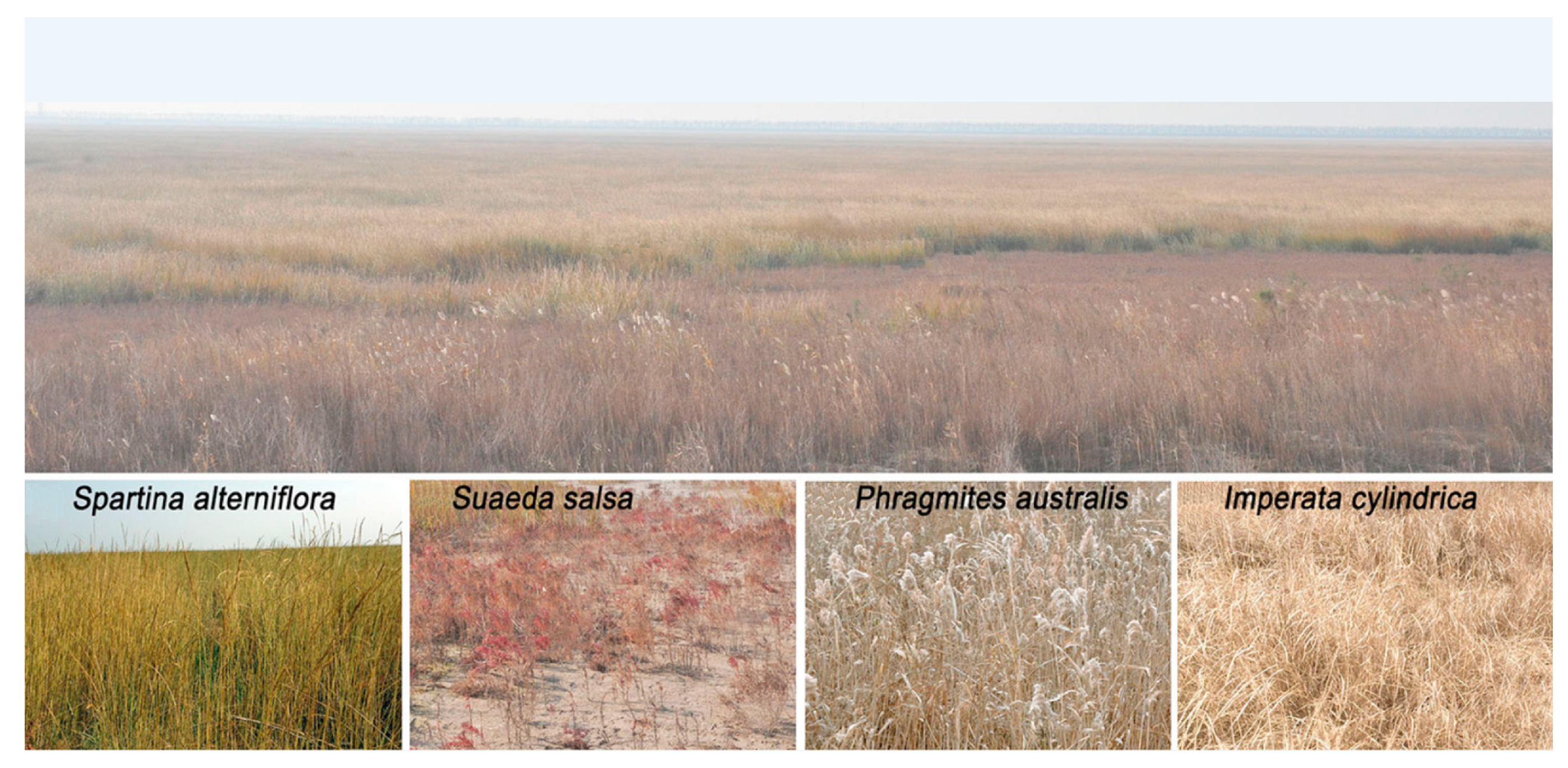
2.1.3. Salt Marshes
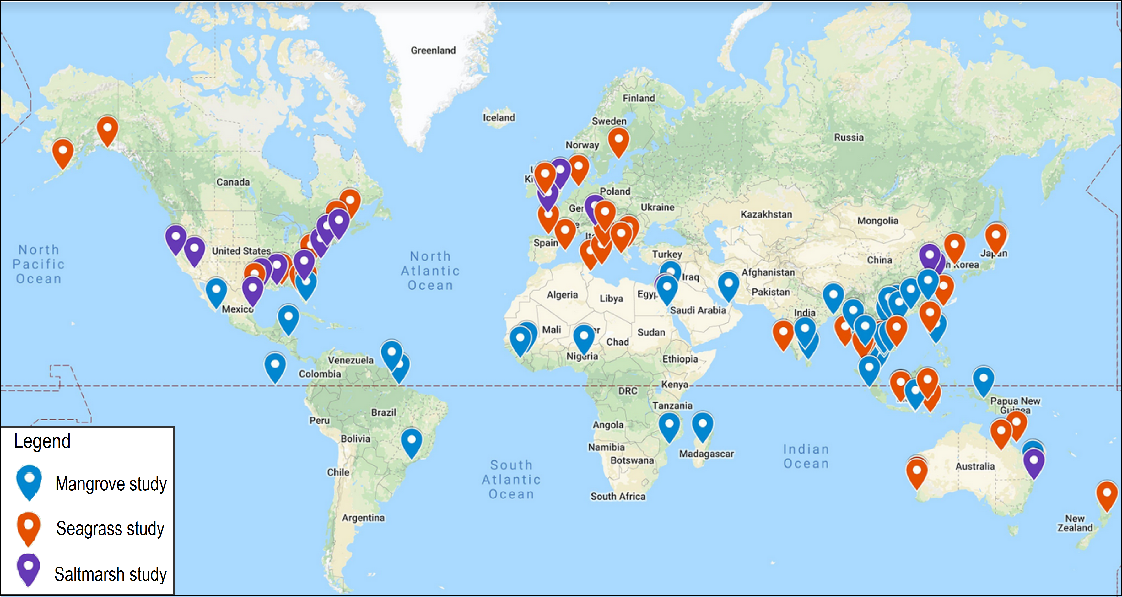
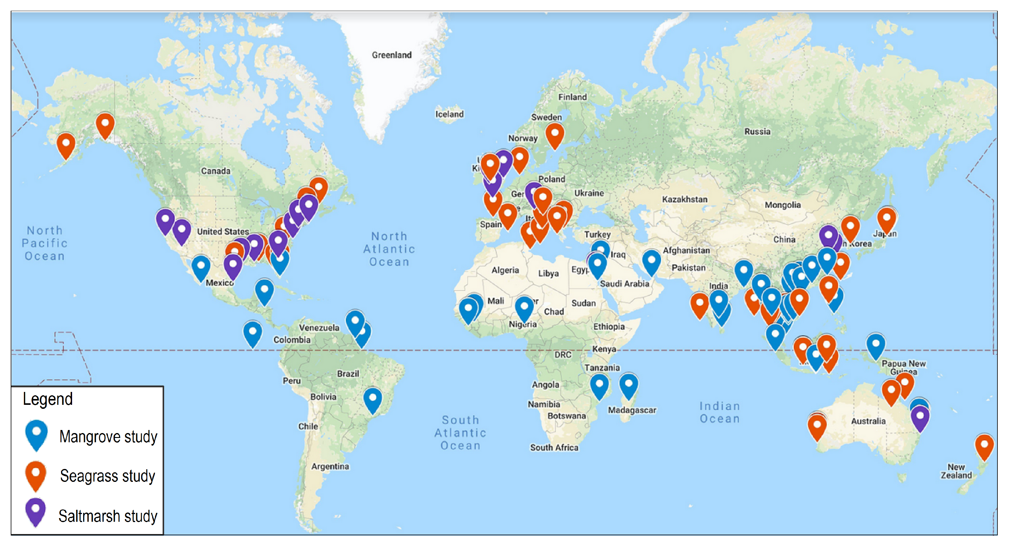
2.2. Inventory, Review, and Comparison of Studies
2.2.1. Summary of Inventory, Datasets, and Methods
2.2.2. Comparison of Studies
2.3. Mangrove Ecosystems
2.3.1. Mapping Mangrove Ecosystems
2.3.2. Monitoring Mangrove Ecosystems
2.4. Seagrass Ecosystems
2.4.1. Mapping Seagrass Ecosystems
2.4.2. Monitoring Seagrass Ecosystems
2.5. Salt Marsh Ecosystems
2.5.1. Mapping Salt Marsh Ecosystems
2.5.2. Monitoring Salt Marsh Ecosystems
3. Future Trends in Mapping and Monitoring BC Ecosystems
3.1. Future Trends in Mapping
3.2. Future Trends in Monitoring
- Improving the mapping accuracy for each time point during the change detection period. Using multisource Earth observation data combined with state-of-the-art machine learning techniques, such as DT ensemble learning, i.e., RFs, rotation forests, and canonical correlation forests [236,237], may improve the mapping accuracy in certain periods.
- In case of a lack of ground truth data in the past, new accuracy metrics should be developed. Limited training data and data incompleteness are common in remote sensing, especially in large-scale time-series datasets. Further, fundamental technologies in remote sensing can deal with limited training data through novel detection techniques, such as transfer learning approaches with deep CNN for image classification [238,239].
- Addressing the best combination of multiple sensors with different techniques for change detection. Because each SAR and optical sensor has its own characteristics in reflecting BC ecosystems, the integration of different remotely-sensed data can offer a number of improvements in accuracy and data acquisition issues in monitoring BC ecosystems. However, the processing time over large areas involved in time-series image analysis should be taken into account [11]. Thus, more research on multiple sensor for monitoring BC ecosystems is needed in the future.
- Developing a standard framework for change detection assessment to enhance the reliability of change detection and to automate the image processing throughout the world. In this context, high performance computing (HPC) facilitates the process, and programming skills are required. This allows researchers to update automatically and re-use classification algorithms, making research faster and expanding the boundaries of BC research [240].
- Understanding the rate of change and the drivers of BC ecosystems. Quantifying the diversity of drivers of BC ecosystems’ changes is important for policy implementations for sustainable conservation and management all over the world [19]. Using combined multitemporal and multi-sensor data can help quantify the key drivers of coastal ecosystem changes.
4. Concluding Remarks
Author Contributions
Funding
Conflicts of Interest
References
- Wolanski, E.; Brinson, M.M.; Cahoon, D.R.; Perillo, G.M.E. Coastal Wetlands: An Integrated Ecosystem Approach, 1st ed.; Elsevier: Amsterdam, The Netherlands, 2009; Chapters 1–57. [Google Scholar]
- Fourqurean, J.W.; Duarte, C.M.; Kennedy, H.; Marbà, N.; Holmer, M.; Mateo, M.A.; Apostolaki, E.T.; Kendrick, G.A.; Krause-Jensen, D.; McGlathery, K.J.; et al. Seagrass ecosystems as a globally significant carbon stock. Nat. Geosci. 2012, 5, 505–509. [Google Scholar] [CrossRef]
- Donato, D.C.; Kauffman, J.B.; Murdiyarso, D.; Kurnianto, S.; Stidham, M.; Kanninen, M. Mangroves among the most carbon-rich forests in the tropics. Nat. Geosci. 2011, 4, 293–297. [Google Scholar] [CrossRef]
- Barbier, E.B.; Hacker, S.D.; Kennedy, C.; Koch, E.W.; Stier, A.C.; Silliman, B.R. The value of estuarine and coastal ecosystem services. Ecol. Monogr. 2011, 81, 169–193. [Google Scholar] [CrossRef]
- Pham, T.D.; Yoshino, K. Impacts of mangrove management systems on mangrove changes in the Northern Coast of Vietnam. Tropics 2016, 24, 141–151. [Google Scholar] [CrossRef]
- Lovelock, C.E.; Cahoon, D.R.; Friess, D.A.; Guntenspergen, G.R.; Krauss, K.W.; Reef, R.; Rogers, K.; Saunders, M.L.; Sidik, F.; Swales, A.; et al. The vulnerability of Indo-Pacific mangrove forests to sea-level rise. Nature 2015, 526, 559–563. [Google Scholar] [CrossRef]
- Food and Agriculture Organization. The World’s Mangroves 1980–2005; FAO Forestry Paper; FAO: Rome, Italy, 2007; Volume 153, 77p. [Google Scholar]
- Waycott, M.; Duarte, C.M.; Carruthers, T.J.B.; Orth, R.J.; Dennison, W.C.; Olyarnik, S.; Calladine, A.; Fourqurean, J.W.; Heck, K.L.; Hughes, A.R.; et al. Accelerating loss of seagrasses across the globe threatens coastal ecosystems. Proc. Natl. Acad. Sci. USA 2009, 106, 12377–12381. [Google Scholar] [CrossRef] [PubMed]
- Valiela, I.; Kinney, E.; Culberston, J.; Peacock, E. Global losses of mangroves and salt marshes. In Global Loss of Coastal Habitats: Rates, Causes and Consequences; Duarte, C.M., Ed.; Fundacion BBVA: Bilbao, Spain, 2009; pp. 109–142. [Google Scholar]
- Hossain, M.; Bujang, J.; Zakaria, M.; Hashim, M. The application of remote sensing to seagrass ecosystems: An overview and future research prospects. Int. J. Remote Sens. 2015, 36, 61–114. [Google Scholar] [CrossRef]
- Pham, T.D.; Yokoya, N.; Bui, D.T.; Yoshino, K.; Friess, D.A. Remote Sensing Approaches for Monitoring Mangrove Species, Structure, and Biomass: Opportunities and Challenges. Remote Sens. 2019, 11, 230. [Google Scholar] [CrossRef]
- Pettorelli, N.; Schulte to Bühne, H.; Tulloch, A.; Dubois, G.; Macinnis-Ng, C.; Queirós, A.M.; Keith, D.A.; Wegmann, M.; Schrodt, F.; Stellmes, M.; et al. Satellite remote sensing of ecosystem functions: Opportunities, challenges and way forward. Remote Sens. Ecol. Conserv. 2018, 4, 71–93. [Google Scholar] [CrossRef]
- Gu, J.; Wang, Z.; Kuen, J.; Ma, L.; Shahroudy, A.; Shuai, B.; Liu, T.; Wang, X.; Wang, G.; Cai, J.; et al. Recent advances in convolutional neural networks. Pattern Recognit. 2018, 77, 354–377. [Google Scholar] [CrossRef]
- Mcleod, E.; Chmura, G.L.; Bouillon, S.; Salm, R.; Björk, M.; Duarte, C.M.; Lovelock, C.E.; Schlesinger, W.H.; Silliman, B.R. A blueprint for blue carbon: Toward an improved understanding of the role of vegetated coastal habitats in sequestering CO2. Front. Ecol. Environ. 2011, 9, 552–560. [Google Scholar] [CrossRef]
- Duke, N.C.; Meynecke, J.O.; Dittmann, S.; Ellison, A.M.; Anger, K.; Berger, U.; Cannicci, S.; Diele, K.; Ewel, K.C.; Field, C.D.; et al. A world without mangroves? Science 2007, 317, 41–42. [Google Scholar] [CrossRef] [PubMed]
- Darmawan, S.; Takeuchi, W.; Vetrita, Y.; Wikantika, K.; Sari, D.K. Impact of topography and tidal height on ALOS palsar polarimetric measurements to estimate aboveground biomass of mangrove forest in Indonesia. J. Sens. 2015. [Google Scholar] [CrossRef]
- Spalding, M. World Atlas of Mangroves; Routledge: Abington, UK, 2010. [Google Scholar]
- Bunting, P.; Rosenqvist, A.; Lucas, R.M.; Rebelo, L.M.; Hilarides, L.; Thomas, N.; Hardy, A.; Itoh, T.; Shimada, M.; Finlayson, C.M. The Global Mangrove Watch—A New 2010 Global Baseline of Mangrove Extent. Remote Sens. 2018, 10, 1669. [Google Scholar] [CrossRef]
- Richards, D.R.; Friess, D.A. Rates and drivers of mangrove deforestation in Southeast Asia, 2000–2012. Proc. Natl. Acad. Sci. USA 2016, 113, 344–349. [Google Scholar] [CrossRef] [PubMed]
- Tien Dat, P.; Yoshino, K. Mangrove analysis using ALOS imagery in Hai Phong City, Vietnam. Proc. SPIE Remote Sens. Mar. Environ. II 2012, 85250U. [Google Scholar] [CrossRef]
- Mtwana Nordlund, L.; Koch, E.W.; Barbier, E.B.; Creed, J.C. Seagrass Ecosystem Services and Their Variability across Genera and Geographical Regions. PLoS ONE 2016, 11, e0163091. [Google Scholar] [CrossRef] [PubMed]
- Howard, J.; Hoyt, S.; Isensee, K.; Pidgeon, E.; Telszewski, M. Coastal Blue Carbon: Methods for Assessing Carbon Stocks And Emissions Factors in Mangroves, Tidal Salt Marshes, and Seagrass Meadows; Intergovernmental Oceanographic Commission of UNESCO, International Union for Conservation of Nature: Arlington, VA, USA, 2014; p. 184. [Google Scholar]
- MarbÃ, N.; Arias-Ortiz, A.; MasquÃ, P.; Kendrick, G.A.; Mazarrasa, I.; Bastyan, G.R.; Garcia-Orellana, J.; Duarte, C.M. Impact of seagrass loss and subsequent revegetation on carbon sequestration and stocks. J. Ecol. 2015, 103, 296–302. [Google Scholar] [CrossRef]
- Thang, H.N.; Yoshino, K.; Hoang Son, T.P. Seagrass mapping using ALOS AVNIR-2 data in Lap An Lagoon, Thua Thien Hue, Viet Nam. Proc. SPIE Remote Sens. Mar. Environ. II 2012, 85250S. [Google Scholar] [CrossRef]
- Lugendo, B. Mangroves, Salt Marshes and Seagrass Beds. In The Regional State of the Coast Report: Western Indian Ocean, 1st ed.; Paula, J., Ed.; UNEP and WIOMSA: New York, NY, USA, 2015; pp. 21–23. [Google Scholar]
- Zedler, J.B.; Kercher, S. Wetland resources: Status, trends, ecosystem services, and restorability. Annu. Rev. Environ. Resour. 2005, 30, 39–74. [Google Scholar] [CrossRef]
- Gedan, K.B.; Silliman, B.R.; Bertness, M.D. Centuries of human-driven change in salt marsh ecosystems. Annu. Rev. Mar. Sci. 2009, 1, 117–141. [Google Scholar] [CrossRef] [PubMed]
- Morris, J.T.; Sundareshwar, P.; Nietch, C.T.; Kjerfve, B.; Cahoon, D.R. Responses of coastal wetlands to rising sea level. Ecology 2002, 83, 2869–2877. [Google Scholar] [CrossRef]
- Sun, C.; Liu, Y.; Zhao, S.; Zhou, M.; Yang, Y.; Li, F. Classification mapping and species identification of salt marshes based on a short-time interval NDVI time-series from HJ-1 optical imagery. Int. J. Appl. Earth Obs. Geoinf. 2016, 45, 27–41. [Google Scholar] [CrossRef]
- Dehvari, A.; Heck, R. Comparison of object-based and pixel based infrared airborne image classification methods using DEM thematic layer. J. Geogr. Reg. Plan. 2009, 2, 86–96. [Google Scholar]
- Navulur, K. Multispectral Image Analysis Using the Object-Oriented Paradigm; CRC Press: Boca Raton, FL, USA, 2007. [Google Scholar]
- Kovacs, J.; de Santiago, F.; Bastien, J.; Lafrance, P. An Assessment of Mangroves in Guinea, West Africa, Using a Field and Remote Sensing Based Approach. Wetlands 2010, 30, 773–782. [Google Scholar] [CrossRef]
- Salami, A.T.; Akinyede, J.; de Gier, A. A preliminary assessment of NigeriaSat-1 for sustainable mangrove forest monitoring. Int. J. Appl. Earth Obs. Geoinf. 2010, 12, S18–S22. [Google Scholar] [CrossRef]
- Yu, X.; Shao, H.B.; Liu, D.-Z.; Zhao, X.H. Applying Neural Network Classification to Obtain Mangrove Landscape Characteristics for Monitoring the Travel Environment Quality on the Beihai Coast of Guangxi, P. R. China. CLEAN Soil Air Water 2010, 38, 289–295. [Google Scholar] [CrossRef]
- Alatorre, L.C.; Sánchez-Andrés, R.; Cirujano, S.; Beguería, S.; Sánchez-Carrillo, S. Identification of Mangrove Areas by Remote Sensing: The ROC Curve Technique Applied to the Northwestern Mexico Coastal Zone Using Landsat Imagery. Remote Sens. 2011, 3, 1568–1583. [Google Scholar] [CrossRef]
- Long, J.B.; Giri, C. Mapping the Philippines’ Mangrove Forests Using Landsat Imagery. Sensors 2011, 11, 2972–2981. [Google Scholar] [CrossRef]
- Satyanarayana, B.; Koedam, N.; De Smet, K.; Di Nitto, D.; Bauwens, M.; Jayatissa, L.P.; Cannicci, S.; Dahdouh-Guebas, F. Long-term mangrove forest development in Sri Lanka: Early predictions evaluated against outcomes using VHR remote sensing and VHR ground-truth data. Mar. Ecol. Prog. Ser. 2011, 443, 51–63. [Google Scholar] [CrossRef]
- Satyanarayana, B.; Mohamad, K.A.; Idris, I.F.; Husain, M.L.; Dahdouh-Guebas, F. Assessment of mangrove vegetation based on remote sensing and ground-truth measurements at Tumpat, Kelantan Delta, East Coast of Peninsular Malaysia. Int. J. Remote Sens. 2011, 32, 1635–1650. [Google Scholar] [CrossRef]
- Beh Boon, C.; Jafri, M.Z.M.; Lim Hwee, S. Mangrove mapping in Penang Island by using Artificial Neural Network technique. In Proceedings of the 2011 IEEE Conference on Open Systems (ICOS), Langkawi, Malaysia, 25–28 September 2011; pp. 245–249. [Google Scholar]
- Dat, P.T.; Yoshino, K. Monitoring Mangrove Forest using Multi-temporal Satellite Data in the Northern Coast of Vietnam. In Proceedings of the The 32nd Asian Conference on Remote Sensing, Taipei, Taiwan, 3–7 October 2011. [Google Scholar]
- Giri, C.; Ochieng, E.; Tieszen, L.L.; Zhu, Z.; Shingh, A.; Loveland, T. Status and distribution of mangrove forests of the world using earth observation satellite data. Glob. Ecol. Biogeogr. 2011, 20, 154–159. [Google Scholar] [CrossRef]
- Nandy, S.; Kushwaha, S. Study on the utility of IRS 1D LISS-III data and the classification techniques for mapping of Sunderban mangroves. J. Coast. Conserv. 2011, 15, 123–137. [Google Scholar] [CrossRef]
- Heumann, B.W. An Object-Based Classification of Mangroves Using a Hybrid Decision Tree—Support Vector Machine Approach. Remote Sens. 2011, 3, 2440–2460. [Google Scholar] [CrossRef]
- Srinivasa Kumar, T.; Mahendra, R.; Nayak, S.; Radhakrishnan, K.; Sahu, K. Identification of hot spots and well managed areas of Pichavaram mangrove using Landsat TM and Resourcesat—1 LISS IV: An example of coastal resource conservation along Tamil Nadu Coast, India. J. Coast. Conserv. 2011, 16, 1–12. [Google Scholar] [CrossRef]
- Chadwick, J. Integrated LiDAR and IKONOS multispectral imagery for mapping mangrove distribution and physical properties. Int. J. Remote Sens. 2011, 32, 6765–6781. [Google Scholar] [CrossRef]
- Rocha de Souza Pereira, F.; Kampel, M.; Cunha-Lignon, M. Mapping of mangrove forests on the southern coast of São Paulo, Brazil, using synthetic aperture radar data from ALOS/PALSAR. Remote Sens. Lett. 2011, 3, 567–576. [Google Scholar] [CrossRef]
- Kirui, K.B.; Kairo, J.G.; Bosire, J.; Viergever, K.M.; Rudra, S.; Huxham, M.; Briers, R.A. Mapping of mangrove forest land cover change along the Kenya coastline using Landsat imagery. Ocean Coast. Manag. 2013, 83, 19–24. [Google Scholar] [CrossRef]
- Vo, Q.; Oppelt, N.; Leinenkugel, P.; Kuenzer, C. Remote Sensing in Mapping Mangrove Ecosystems—An Object-Based Approach. Remote Sens. 2013, 5, 183–201. [Google Scholar] [CrossRef]
- Cardoso, G.F.; Souza, C.; Souza-Filho, P.W.M. Using spectral analysis of Landsat-5 TM images to map coastal wetlands in the Amazon River mouth, Brazil. Wetl. Ecol. Manag. 2014, 22, 79–92. [Google Scholar] [CrossRef]
- Kamal, M.; Phinn, S.; Johansen, K. Characterizing the Spatial Structure of Mangrove Features for Optimizing Image-Based Mangrove Mapping. Remote Sens. 2014, 6, 984–1006. [Google Scholar] [CrossRef]
- Jones, T.; Ratsimba, H.; Ravaoarinorotsihoarana, L.; Cripps, G.; Bey, A. Ecological Variability and Carbon Stock Estimates of Mangrove Ecosystems in Northwestern Madagascar. Forests 2014, 5, 177–205. [Google Scholar] [CrossRef]
- Singh, S.K.; Srivastava, P.K.; Gupta, M.; Thakur, J.K.; Mukherjee, S. Appraisal of land use/land cover of mangrove forest ecosystem using support vector machine. Environ. Earth Sci. 2014, 71, 2245–2255. [Google Scholar] [CrossRef]
- Kamal, M.; Phinn, S.; Johansen, K. Object-Based Approach for Multi-Scale Mangrove Composition Mapping Using Multi-Resolution Image Datasets. Remote Sens. 2015, 7, 4753–4783. [Google Scholar] [CrossRef]
- Giardino, C.; Bresciani, M.; Fava, F.; Matta, E.; Brando, V.; Colombo, R. Mapping Submerged Habitats and Mangroves of Lampi Island Marine National Park (Myanmar) from in Situ and Satellite Observations. Remote Sens. 2016, 8, 2. [Google Scholar] [CrossRef]
- Jones, T.; Glass, L.; Gandhi, S.; Ravaoarinorotsihoarana, L.; Carro, A.; Benson, L.; Ratsimba, H.; Giri, C.; Randriamanatena, D.; Cripps, G. Madagascar’s Mangroves: Quantifying Nation-Wide and Ecosystem Specific Dynamics, and Detailed Contemporary Mapping of Distinct Ecosystems. Remote Sens. 2016, 8, 106. [Google Scholar] [CrossRef]
- Aslan, A.; Rahman, A.F.; Warren, M.W.; Robeson, S.M. Mapping spatial distribution and biomass of coastal wetland vegetation in Indonesian Papua by combining active and passive remotely sensed data. Remote Sens. Environ. 2016, 183, 65–81. [Google Scholar] [CrossRef]
- Chen, B.; Xiao, X.; Li, X.; Pan, L.; Doughty, R.; Ma, J.; Dong, J.; Qin, Y.; Zhao, B.; Wu, Z.; et al. A mangrove forest map of China in 2015: Analysis of time series Landsat 7/8 and Sentinel-1A imagery in Google Earth Engine cloud computing platform. ISPRS J. Photogramm. Remote Sens. 2017, 131, 104–120. [Google Scholar] [CrossRef]
- Zhang, X.; Treitz, P.M.; Chen, D.; Quan, C.; Shi, L.; Li, X. Mapping mangrove forests using multi-tidal remotely-sensed data and a decision-tree-based procedure. Int. J. Appl. Earth Obs. Geoinf. 2017, 62, 201–214. [Google Scholar] [CrossRef]
- Almahasheer, H. Spatial coverage of mangrove communities in the Arabian Gulf. Environ. Monit. Assess. 2018, 190, 85. [Google Scholar] [CrossRef]
- Kiefer, R.W.; Lillesand, M.T. Remote Sensing and Image Interpretation, 6th ed.; Wiley: Hoboken, NJ, USA, 2007; 804p. [Google Scholar]
- Calzadilla Pérez, A.; Damen, M.C.J.; Geneletti, D.; Hobma, T.W. Monitoring a Recent Delta Formation in a Tropical Coastal Wetland Using Remote Sensing and GIS. Case Study: Guapo River Delta, Laguna de Tacarigua, Venezuela. Environ. Dev. Sustain. 2002, 4, 201–219. [Google Scholar] [CrossRef]
- Yagoub, M.; Kolan, G. Monitoring coastal zone land use and land cover changes of Abu Dhabi using remote sensing. J. Indian Soc. Remote Sens. 2006, 34, 57–68. [Google Scholar] [CrossRef]
- Giri, C.; Pengra, B.; Zhu, Z.; Singh, A.; Tieszen, L.L. Monitoring mangrove forest dynamics of the Sundarbans in Bangladesh and India using multi-temporal satellite data from 1973 to 2000. Estuar. Coast. Shelf Sci. 2007, 73, 91–100. [Google Scholar] [CrossRef]
- Everitt, J.H.; Yang, C.; Judd, F.W.; Summy, K.R. Use of Archive Aerial Photography for Monitoring Black Mangrove Populations. J. Coast. Res. 2010, 649–653. [Google Scholar] [CrossRef]
- Rakotomavo, A.; Fromard, F. Dynamics of mangrove forests in the Mangoky River delta, Madagascar, under the influence of natural and human factors. For. Ecol. Manag. 2010, 259, 1161–1169. [Google Scholar] [CrossRef]
- Kanniah, K.; Sheikhi, A.; Cracknell, A.; Goh, H.; Tan, K.; Ho, C.; Rasli, F. Satellite Images for Monitoring Mangrove Cover Changes in a Fast Growing Economic Region in Southern Peninsular Malaysia. Remote Sens. 2015, 7, 14360–14385. [Google Scholar] [CrossRef]
- Abdul Aziz, A.; Phinn, S.; Dargusch, P.; Omar, H.; Arjasakusuma, S. Assessing the potential applications of Landsat image archive in the ecological monitoring and management of a production mangrove forest in Malaysia. Wetl. Ecol. Manag. 2015, 23, 1049–1066. [Google Scholar] [CrossRef]
- Lam-Dao, N.; Pham-Bach, V.; Nguyen-Thanh, M.; Pham-Thi, M.T.; Hoang-Phi, P. Change Detection of Land use and Riverbank in Mekong Delta, Vietnam using Time Series Remotely Sensed Data. J. Resour. Ecol. 2011, 2, 370–374. [Google Scholar] [CrossRef]
- Nguyen, H.H.; McAlpine, C.; Pullar, D.; Johansen, K.; Duke, N.C. The relationship of spatial–temporal changes in fringe mangrove extent and adjacent land-use: Case study of Kien Giang coast, Vietnam. Ocean Coast. Manag. 2013, 76, 12–22. [Google Scholar] [CrossRef]
- Rodriguez, W.; Feller, I.C.; Cavanaugh, K.C. Spatio-temporal changes of a mangrove–saltmarsh ecotone in the northeastern coast of Florida, USA. Glob. Ecol. Conserv. 2016, 7, 245–261. [Google Scholar] [CrossRef]
- Kesgin, B.; Nurlu, E. Land cover changes on the coastal zone of Candarli Bay, Turkey using remotely sensed data. Environ. Monit. Assess. 2009, 157, 89–96. [Google Scholar] [CrossRef] [PubMed]
- Aschbacher, J.; Ofren, R.; Delsol, J.P.; Suselo, T.B.; Vibulsresth, S.; Charrupat, T. An integrated comparative approach to mangrove vegetation mapping using advanced remote sensing and GIS technologies: Preliminary results. Hydrobiologia 1995, 295, 285–294. [Google Scholar] [CrossRef]
- Binh Vromant, N.; Hung, N.T.; Hens, L.; Boon, E.K. Land cover changes between 1968 and 2003 in Cai Nuoc, Ca Mau Peninsula, Vietnam. Environ. Dev. Sustain. 2005, 7, 519–536. [Google Scholar] [CrossRef]
- Valderrama-Landeros, L.; Flores-de Santiago, F.; Kovacs, J.M.; Flores-Verdugo, F. An assessment of commonly employed satellite-based remote sensors for mapping mangrove species in Mexico using an NDVI-based classification scheme. Environ. Monit. Assess. 2017, 190, 23. [Google Scholar] [CrossRef] [PubMed]
- Satyanarayana, B.; Thierry, D.; Seen, L.; Raman, A.V.; Muthusankar, G. Remote Sensing In Mangrove Research—Relationship between Vegetation Indices And Dendrometric Parameters: A Case For Coringa, East Coast of India. 2001. Available online: https://crisp.nus.edu.sg/ acrs2001/pdf/160LOSEE.PDF (accessed on 15 January 2019).
- Lee, T.M.; Yeh, H.C. Applying remote sensing techniques to monitor shifting wetland vegetation: A case study of Danshui River estuary mangrove communities, Taiwan. Ecol. Eng. 2009, 35, 487–496. [Google Scholar] [CrossRef]
- Conchedda, G.; Durieux, L.; Mayaux, P. An object-based method for mapping and change analysis in mangrove ecosystems. ISPRS J. Photogramm. Remote Sens. 2008, 63, 578–589. [Google Scholar] [CrossRef]
- Zingaretti, P.; Frontoni, E.; Malinverni, E.; Mancini, A. A Hybrid Approach to Land Cover Classification from Multi Spectral Images. In Image Analysis and Processing—ICIAP 2009; Foggia, P., Sansone, C., Vento, M., Eds.; Springer: Berlin/Heidelberg, Germany, 2009; Volume 5716, pp. 500–508. [Google Scholar]
- Li, M.S.; Mao, L.J.; Shen, W.J.; Liu, S.Q.; Wei, A.S. Change and fragmentation trends of Zhanjiang mangrove forests in southern China using multi-temporal Landsat imagery (1977–2010). Estuar. Coast. Shelf Sci. 2013, 130, 111–120. [Google Scholar] [CrossRef]
- Rogers, K.; Lymburner, L.; Salum, R.; Brooke, B.P.; Woodroffe, C.D. Mapping of mangrove extent and zonation using high and low tide composites of Landsat data. Hydrobiologia 2017, 803, 49–68. [Google Scholar] [CrossRef]
- Bullock, E.L.; Fagherazzi, S.; Nardin, W.; Vo-Luong, P.; Nguyen, P.; Woodcock, C.E. Temporal patterns in species zonation in a mangrove forest in the Mekong Delta, Vietnam, using a time series of Landsat imagery. Cont. Shelf Res. 2017, 147, 144–154. [Google Scholar] [CrossRef]
- Tran Thi, V.; Tien Thi Xuan, A.; Phan Nguyen, H.; Dahdouh-Guebas, F.; Koedam, N. Application of remote sensing and GIS for detection of long-term mangrove shoreline changes in Mui Ca Mau, Vietnam. Biogeosciences 2014, 11, 3781–3795. [Google Scholar] [CrossRef]
- Liu, M.; Zhang, H.; Lin, G.; Lin, H.; Tang, D. Zonation and Directional Dynamics of Mangrove Forests Derived from Time-Series Satellite Imagery in Mai Po, Hong Kong. Sustainability 2018, 10, 1913. [Google Scholar] [CrossRef]
- Thomas, N.; Lucas, R.; Itoh, T.; Simard, M.; Fatoyinbo, L.; Bunting, P.; Rosenqvist, A. An approach to monitoring mangrove extents through time-series comparison of JERS-1 SAR and ALOS PALSAR data. Wetl. Ecol. Manag. 2015, 23, 3–17. [Google Scholar] [CrossRef]
- Pham, T.D.; Yoshino, K.; Kaida, N. Monitoring Mangrove Forest Changes in Cat Ba Biosphere Reserve Using ALOS PALSAR Imagery and a GIS-Based Support Vector Machine Algorithm. In Advances and Applications in Geospatial Technology and Earth Resources; Tien Bui, D., Ngoc Do, A., Bui, H.B., Hoang, N.D., Eds.; Springer International Publishing: Cham, Switzerland, 2018; pp. 103–118. [Google Scholar]
- Pattanaik, C.; Narendra Prasad, S. Assessment of aquaculture impact on mangroves of Mahanadi delta (Orissa), East coast of India using remote sensing and GIS. Ocean Coast. Manag. 2011, 54, 789–795. [Google Scholar] [CrossRef]
- Rahman, A.F.; Dragoni, D.; Didan, K.; Barreto-Munoz, A.; Hutabarat, J.A. Detecting large scale conversion of mangroves to aquaculture with change point and mixed-pixel analyses of high-fidelity MODIS data. Remote Sens. Environ. 2013, 130, 96–107. [Google Scholar] [CrossRef]
- Chen, C.F.; Son, N.T.; Chang, N.B.; Chen, C.R.; Chang, L.Y.; Valdez, M.; Centeno, G.; Thompson, C.; Aceituno, J. Multi-Decadal Mangrove Forest Change Detection and Prediction in Honduras, Central America, with Landsat Imagery and a Markov Chain Model. Remote Sens. 2013, 5, 6408–6426. [Google Scholar] [CrossRef]
- Lucas, R.; Rebelo, L.M.; Fatoyinbo, L.; Rosenqvist, A.; Itoh, T.; Shimada, M.; Simard, M.; Souza-Filho, P.W.; Thomas, N.; Trettin, C.; et al. Contribution of L-band SAR to systematic global mangrove monitoring. Mar. Freshw. Res. 2014, 65, 589–603. [Google Scholar] [CrossRef]
- Webb, E.L.; Jachowski, N.R.A.; Phelps, J.; Friess, D.A.; Than, M.M.; Ziegler, A.D. Deforestation in the Ayeyarwady Delta and the conservation implications of an internationally-engaged Myanmar. Glob. Environ. Chang. 2014, 24, 321–333. [Google Scholar] [CrossRef]
- Vu, T.D.; Takeuchi, W.; Van, N.A. Carbon Stock Calculating and Forest Change Assessment Toward REDD+ Activities for The Mangrove Forest in Vietnam. Trans. Japan Soc. Aeronaut. Space Sci. Aerosp. Technol. Japan 2014, 12, Pn_23–Pn_31. [Google Scholar] [CrossRef]
- Giri, C.; Long, J.; Abbas, S.; Murali, R.M.; Qamer, F.M.; Pengra, B.; Thau, D. Distribution and dynamics of mangrove forests of South Asia. J. Environ. Manag. 2015, 148, 101–111. [Google Scholar] [CrossRef]
- Van, T.T.; Wilson, N.; Thanh-Tung, H.; Quisthoudt, K.; Quang-Minh, V.; Xuan-Tuan, L.; Dahdouh-Guebas, F.; Koedam, N. Changes in mangrove vegetation area and character in a war and land use change affected region of Vietnam (Mui Ca Mau) over six decades. Acta Oecol. 2015, 63, 71–81. [Google Scholar] [CrossRef]
- Hamilton, S.E.; Lovette, J. Ecuador’s Mangrove Forest Carbon Stocks: A Spatiotemporal Analysis of Living Carbon Holdings and Their Depletion since the Advent of Commercial Aquaculture. PLoS ONE 2015, 10, e0118880. [Google Scholar] [CrossRef] [PubMed]
- Pham, T.D.; Yoshino, K. Mangrove Mapping and Change Detection Using Multi-temporal Landsat imagery in Hai Phong city, Vietnam. In Proceedings of the International Symposium on Cartography in Internet and Ubiquitous Environments 2015, Tokyo, Japan, 17–19 March 2015. [Google Scholar]
- Nguyen-Thanh, S.; Chi-Farn, C.; Ni-Bin, C.; Cheng-Ru, C.; Ly-Yu, C.; Bui-Xuan, T. Mangrove Mapping and Change Detection in Ca Mau Peninsula, Vietnam, Using Landsat Data and Object-Based Image Analysis. IEEE J. Sel. Top. Appl. Earth Obs. Remote Sens. 2015, 8, 503–510. [Google Scholar] [CrossRef]
- Shapiro, A.; Trettin, C.; Küchly, H.; Alavinapanah, S.; Bandeira, S. The Mangroves of the Zambezi Delta: Increase in Extent Observed via Satellite from 1994 to 2013. Remote Sens. 2015, 7, 16504–16518. [Google Scholar] [CrossRef]
- Son, N.T.; Thanh, B.X.; Da, C.T. Monitoring Mangrove Forest Changes from Multi-temporal Landsat Data in Can Gio Biosphere Reserve, Vietnam. Wetlands 2016, 36, 565–576. [Google Scholar] [CrossRef]
- William, N.; Silvia, L.; Valerie, P.; Cristina, R.M.; Cristina, E.W.; Sergio, F. Dynamics of a fringe mangrove forest detected by Landsat images in the Mekong River Delta, Vietnam. Earth Surf. Process. Landforms 2016, 41, 2024–2037. [Google Scholar] [CrossRef]
- Viennois, G.; Proisy, C.; Féret, J.B.; Prosperi, J.; Sidik, F.; Suhardjono; Rahmania, R.; Longépé, N.; Germain, O.; Gaspar, P. Multitemporal Analysis of High-Spatial-Resolution Optical Satellite Imagery for Mangrove Species Mapping in Bali, Indonesia. IEEE J. Sel. Top. Appl. Earth Obs. Remote Sens. 2016, 9, 3680–3686. [Google Scholar] [CrossRef]
- Hauser, L.T.; Nguyen Vu, G.; Nguyen, B.A.; Dade, E.; Nguyen, H.M.; Nguyen, T.T.Q.; Le, T.Q.; Vu, L.H.; Tong, A.T.H.; Pham, H.V. Uncovering the spatio-temporal dynamics of land cover change and fragmentation of mangroves in the Ca Mau peninsula, Vietnam using multi-temporal SPOT satellite imagery (2004–2013). Appl. Geogr. 2017, 86, 197–207. [Google Scholar] [CrossRef]
- Pham, L.T.H.; Brabyn, L. Monitoring mangrove biomass change in Vietnam using SPOT images and an object-based approach combined with machine learning algorithms. ISPRS J. Photogramm. Remote Sens. 2017, 128, 86–97. [Google Scholar] [CrossRef]
- Benson, L.; Glass, L.; Jones, T.; Ravaoarinorotsihoarana, L.; Rakotomahazo, C. Mangrove Carbon Stocks and Ecosystem Cover Dynamics in Southwest Madagascar and the Implications for Local Management. Forests 2017, 8, 190. [Google Scholar] [CrossRef]
- Proisy, C.; Viennois, G.; Sidik, F.; Andayani, A.; Enright, J.A.; Guitet, S.; Gusmawati, N.; Lemonnier, H.; Muthusankar, G.; Olagoke, A.; et al. Monitoring mangrove forests after aquaculture abandonment using time series of very high spatial resolution satellite images: A case study from the Perancak estuary, Bali, Indonesia. Mar. Pollut. Bull. 2018, 131, 61–71. [Google Scholar] [CrossRef]
- Mondal, P.; Trzaska, S.; de Sherbinin, A. Landsat-Derived Estimates of Mangrove Extents in the Sierra Leone Coastal Landscape Complex during 1990–2016. Sensors 2018, 18, 12. [Google Scholar] [CrossRef] [PubMed]
- Abdel-Hamid, A.; Dubovyk, O.; Abou El-Magd, I.; Menz, G. Mapping Mangroves Extents on the Red Sea Coastline in Egypt using Polarimetric SAR and High Resolution Optical Remote Sensing Data. Sustainability 2018, 10, 646. [Google Scholar] [CrossRef]
- Islam, M.M.; Borgqvist, H.; Kumar, L. Monitoring Mangrove Forest Landcover Changes in the Coastline of Bangladesh from 1976 to 2015. Geocarto Int. 2018. [Google Scholar] [CrossRef]
- Wang, M.; Cao, W.; Guan, Q.; Wu, G.; Wang, F. Assessing changes of mangrove forest in a coastal region of southeast China using multi-temporal satellite images. Estuar. Coast. Shelf Sci. 2018, 207, 283–292. [Google Scholar] [CrossRef]
- Gaw, L.Y.F.; Linkie, M.; Friess, D.A. Mangrove forest dynamics in Tanintharyi, Myanmar from 1989–2014, and the role of future economic and political developments. Singap. J. Trop. Geogr. 2018, 39, 224–243. [Google Scholar] [CrossRef]
- Kovacs, E.; Roelfsema, C.; Lyons, M.; Zhao, S.; Phinn, S. Seagrass habitat mapping: How do Landsat 8 OLI, Sentinel-2, ZY-3A, and Worldview-3 perform? Remote Sens. Lett. 2018, 9, 686–695. [Google Scholar] [CrossRef]
- Koedsin, W.; Intararuang, W.; Ritchie, R.; Huete, A. An Integrated Field and Remote Sensing Method for Mapping Seagrass Species, Cover, and Biomass in Southern Thailand. Remote Sens. 2016, 8, 292. [Google Scholar] [CrossRef]
- Baumstark, R.; Duffey, R.; Pu, R. Mapping seagrass and colonized hard bottom in Springs Coast, Florida using WorldView-2 satellite imagery. Estuar. Coast. Shelf Sci. 2016, 181, 83–92. [Google Scholar] [CrossRef]
- Wicaksono, P. Improving the accuracy of Multispectral-based benthic habitats mapping using image rotations: The application of Principle Component Analysis and Independent Component Analysis. Eur. J. Remote Sens. 2016, 49, 433–463. [Google Scholar] [CrossRef]
- Tamondong, A.M.; Blanco, A.C.; Fortes, M.D.; Nadaoka, K. Mapping of seagrass and other benthic habitats in Bolinao, Pangasinan using Worldview-2 satellite image. In Proceedings of the IGARSS 2013—2013 IEEE International Geoscience and Remote Sensing Symposium, Melbourne, VIC, Australia, 21–26 July 2013; pp. 1579–1582. [Google Scholar] [CrossRef]
- Saunders, M.I.; Bayraktarov, E.; Roelfsema, C.M.; Leon, J.X.; Samper-Villarreal, J.; Phinn, S.R.; Lovelock, C.E.; Mumby, P.J. Spatial and temporal variability of seagrass at Lizard Island, Great Barrier Reef. Bot. Mar. 2015, 58, 35–49. [Google Scholar] [CrossRef]
- Sagawa, T.; Komatsu, T. Simulation of seagrass bed mapping by satellite images based on the radiative transfer model. Ocean Sci. J. 2015, 50, 335–342. [Google Scholar] [CrossRef]
- Knudby, A.; Nordlund, L. Remote sensing of seagrasses in a patchy multi-species environment. Int. J. Remote Sens. 2011, 32, 2227–2244. [Google Scholar] [CrossRef]
- Pu, R.; Bell, S. Mapping seagrass coverage and spatial patterns with high spatial resolution IKONOS imagery. Int. J. Appl. Earth Obs. Geoinf. 2017, 54, 145–158. [Google Scholar] [CrossRef]
- Baumstark, R.; Dixon, B.; Carlson, P.; Palandro, D.; Kolasa, K. Alternative spatially enhanced integrative techniques for mapping seagrass in Florida’s marine ecosystem. Int. J. Remote Sens. 2013, 34, 1248–1264. [Google Scholar] [CrossRef]
- Sagawa, T.; Boisnier, E.; Komatsu, T.; Mustapha, K.B.; Hattour, A.; Kosaka, N.; Miyazaki, S. Using bottom surface reflectance to map coastal marine areas: A new application method for Lyzenga’s model. Int. J. Remote Sens. 2010, 31, 3051–3064. [Google Scholar] [CrossRef]
- Meyer, R.P.; Bell, S.; Levy, K.H.; Meyer, C. Mapping detailed seagrass habitats using satellite imagery. In Proceedings of the 2010 IEEE International Geoscience and Remote Sensing Symposium, Honolulu, HI, USA, 25–30 July 2010; p. 4. [Google Scholar] [CrossRef]
- Fearns, P.R.C.; Klonowski, W.; Babcock, R.C.; England, P.; Phillips, J. Shallow water substrate mapping using hyperspectral remote sensing. Cont. Shelf Res. 2011, 31, 1249–1259. [Google Scholar] [CrossRef]
- Ferreira, M.A.; Andrade, F.; Mendes, R.N.; Paula, J. Use of satellite remote sensing for coastal conservation in the Eastern African Coast: Advantages and shortcomings. Eur. J. Remote Sens. 2012, 45, 293–304. [Google Scholar] [CrossRef]
- Lu, D.; Cho, H.J. An improved water-depth correction algorithm for seagrass mapping using hyperspectral data. Remote Sens. Lett. 2011, 2, 91–97. [Google Scholar] [CrossRef]
- Nobi, E.P.; Thangaradjou, T. Evaluation of the spatial changes in seagrass cover in the lagoons of Lakshadweep islands, India, using IRS LISS III satellite images. Geocarto Int. 2012, 27, 647–660. [Google Scholar] [CrossRef]
- Micallef, A.; Le Bas, T.P.; Huvenne, V.A.I.; Blondel, P.; Hühnerbach, V.; Deidun, A. A multi-method approach for benthic habitat mapping of shallow coastal areas with high-resolution multibeam data. Cont. Shelf Res. 2012, 39–40, 14–26. [Google Scholar] [CrossRef]
- Li, R.; Liu, J.K.; Sukcharoenpong, A.; Yuan, J.; Zhu, H.; Zhang, S. A Systematic Approach toward Detection of Seagrass Patches from Hyperspectral Imagery. Mar. Geod. 2012, 35, 271–286. [Google Scholar] [CrossRef]
- Paulose, N.E.; Dilipan, E.; Thangaradjou, T. Integrating Indian remote sensing multi-spectral satellite and field data to estimate seagrass cover change in the Andaman and Nicobar Islands, India. Ocean Sci. J. 2013, 48, 173–181. [Google Scholar] [CrossRef]
- Pu, R.; Bell, S. A protocol for improving mapping and assessing of seagrass abundance along the West Central Coast of Florida using Landsat TM and EO-1 ALI/Hyperion images. ISPRS J. Photogramm. Remote Sens. 2013, 83, 116–129. [Google Scholar] [CrossRef]
- Borfecchia, F.; Micheli, C.; Carli, F.; De Martis, S.; Gnisci, V.; Piermattei, V.; Belmonte, A.; De Cecco, L.; Martini, S.; Marcelli, M. Mapping Spatial Patterns of Posidonia oceanica Meadows by Means of Daedalus ATM Airborne Sensor in the Coastal Area of Civitavecchia (Central Tyrrhenian Sea, Italy). Remote Sens. 2013, 5, 4877–4899. [Google Scholar] [CrossRef]
- Massot-Campos, M.; Oliver-Codina, G.; Ruano-Amengual, L.; Miro-Julia, M. Texture analysis of seabed images: Quantifying the presence of Posidonia oceanica at Palma Bay. In Proceedings of the 2013 IEEE MTS/IEEE OCEANS, Bergen, Norway, 10–14 June 2013; pp. 1–6. [Google Scholar] [CrossRef]
- Wicaksono, P.; Hafizt, M. Mapping Seagrass from Space: Addressing the Complexity of Seagrass LAI Mapping. Eur. J. Remote Sens. 2013, 46, 18–39. [Google Scholar] [CrossRef]
- Torres-Pulliza, D.; Wilson, J.R.; Darmawan, A.; Campbell, S.J.; Andréfouët, S. Ecoregional scale seagrass mapping: A tool to support resilient MPA network design in the Coral Triangle. Ocean Coast. Manag. 2013, 80, 55–64. [Google Scholar] [CrossRef]
- March, D.; Alós, J.; Cabanellas-Reboredo, M.; Infantes, E.; Jordi, A.; Palmer, M. A Bayesian spatial approach for predicting seagrass occurrence. Estuar. Coast. Shelf Sci. 2013, 131, 206–212. [Google Scholar] [CrossRef]
- Nguyen, D.T.H.; Tripathi, N.K.; Gallardo, W.G.; Tipdecho, T. Coastal and marine ecological changes and fish cage culture development in Phu Quoc, Vietnam (2001 to 2011). Geocarto Int. 2014, 29, 486–506. [Google Scholar] [CrossRef]
- Hogrefe, K.; Ward, D.; Donnelly, T.; Dau, N. Establishing a Baseline for Regional Scale Monitoring of Eelgrass (Zostera marina) Habitat on the Lower Alaska Peninsula. Remote Sens. 2014, 6, 12447–12477. [Google Scholar] [CrossRef]
- Cho, H.J.; Ogashawara, I.; Mishra, D.; White, J.; Kamerosky, A.; Morris, L.; Clarke, C.; Simpson, A.; Banisakher, D. Evaluating Hyperspectral Imager for the Coastal Ocean (HICO) data for seagrass mapping in Indian River Lagoon, FL. GISci. Remote Sens. 2014, 51, 120–138. [Google Scholar] [CrossRef]
- Kim, K.; Choi, J.K.; Ryu, J.H.; Jeong, H.J.; Lee, K.; Park, M.G.; Kim, K.Y. Observation of typhoon-induced seagrass die-off using remote sensing. Estuar. Coast. Shelf Sci. 2015, 154, 111–121. [Google Scholar] [CrossRef]
- Valle, M.; Pala, V.; Lafon, V.; Dehouck, A.; Garmendia, J.M.; Borja, A.; Chust, G. Mapping estuarine habitats using airborne hyperspectral imagery, with special focus on seagrass meadows. Estuar. Coast. Shelf Sci. 2015, 164, 433–442. [Google Scholar] [CrossRef]
- Garcia, R.; Hedley, J.; Tin, H.; Fearns, P. A Method to Analyze the Potential of Optical Remote Sensing for Benthic Habitat Mapping. Remote Sens. 2015, 7, 13157–13189. [Google Scholar] [CrossRef]
- Barrell, J.; Grant, J.; Hanson, A.; Mahoney, M. Evaluating the complementarity of acoustic and satellite remote sensing for seagrass landscape mapping. Int. J. Remote Sens. 2015, 36, 4069–4094. [Google Scholar] [CrossRef]
- Roelfsema, C.; Lyons, M.; Dunbabin, M.; Kovacs, E.M.; Phinn, S. Integrating field survey data with satellite image data to improve shallow water seagrass maps: The role of AUV and snorkeller surveys? Remote Sens. Lett. 2015, 6, 135–144. [Google Scholar] [CrossRef]
- Schubert, P.; Hukriede, W.; Karez, R.; Reusch, T. Mapping and modeling eelgrass Zostera marina distribution in the western Baltic Sea. Mar. Ecol. Prog. Ser. 2015, 522, 79–95. [Google Scholar] [CrossRef]
- Tsujimoto, R.; Terauchi, G.; Sasaki, H.; Sakamoto, S.X.; Sawayama, S.; Sasa, S.; Yagi, H.; Komatsu, T. Damage to seagrass and seaweed beds in Matsushima Bay, Japan, caused by the huge tsunami of the Great East Japan Earthquake on 11 March 2011. Int. J. Remote Sens. 2016, 37, 5843–5863. [Google Scholar] [CrossRef]
- Purnawan, S.; Aulia, F.; Khairuman, T. Using Landsat-8 Imagery Data on Mapping of The Seagrass Distribution in Matahari Island, Pulau Banyak District, Aceh Province, Indonesia. Aceh Int. J. Sci. Technol. 2016, 5, 63–68. [Google Scholar] [CrossRef]
- Uhrin, A.V.; Townsend, P.A. Improved seagrass mapping using linear spectral unmixing of aerial photographs. Estuar. Coast. Shelf Sci. 2016, 171, 11–22. [Google Scholar] [CrossRef]
- Kakuta, S.; Takeuchi, W.; Prathep, A. Seaweed and seagrass mapping in thailand measured using Landsat 8 optical and textural image properties. J. Mar. Sci. Technol. 2016, 24, 1155–1160. [Google Scholar] [CrossRef]
- Pan, Z.; Glennie, C.; Fernandez-Diaz, J.C.; Starek, M. Comparison of bathymetry and seagrass mapping with hyperspectral imagery and airborne bathymetric lidar in a shallow estuarine environment. Int. J. Remote Sens. 2016, 37, 516–536. [Google Scholar] [CrossRef]
- Folmer, E.O.; van Beusekom, J.E.E.; Dolch, T.; Gräwe, U.; van Katwijk, M.M.; Kolbe, K.; Philippart, C.J.M. Consensus forecasting of intertidal seagrass habitat in the Wadden Sea. J. Appl. Ecol. 2016, 53, 1800–1813. [Google Scholar] [CrossRef]
- Bonin-Font, F.; Campos, M.M.; Codina, G.O. Towards Visual Detection, Mapping and Quantification of Posidonia Oceanica using a Lightweight AUV. IFAC-PapersOnLine 2016, 49, 500–505. [Google Scholar] [CrossRef]
- Pe’eri, S.; Morrison, J.R.; Short, F.; Mathieson, A.; Lippmann, T. Eelgrass and Macroalgal Mapping to Develop Nutrient Criteria in New Hampshire’s Estuaries using Hyperspectral Imagery. J. Coast. Res. 2016, 76, 209–218. [Google Scholar] [CrossRef]
- da Silva, G.C.M.; de Souza, F.E.S.; Marinho-Soriano, E. Application of ALOS AVNIR-2 for the detection of seaweed and seagrass beds on the northeast of Brazil. Int. J. Remote Sens. 2017, 38, 662–678. [Google Scholar] [CrossRef]
- Hedley, J.D.; Russell, B.J.; Randolph, K.; Perez-Castro, M.A.; Vasquez-Elizondo, R.M.; Enriquez, S.; Dierssen, H.M. Remote Sensing of Seagrass Leaf Area Index and Species: The Capability of a Model Inversion Method Assessed by Sensitivity Analysis and Hyperspectral Data of Florida Bay. Front. Mar. Sci. 2017, 4, 362. [Google Scholar] [CrossRef]
- Traganos, D.; Cerra, D.; Reinartz, P. Cubesat-derived detection of seagrasses using planet imagery following unmixing-based denoising: Is small the next big? ISPRS Int. Arch. Photogramm. Remote Sens. Spat. Inf. Sci. 2017, XLII-1/W1, 283–287. [Google Scholar] [CrossRef]
- Ferretti, R.; Bibuli, M.; Caccia, M.; Chiarella, D.; Odetti, A.; Ranieri, A.; Zereik, E.; Bruzzone, G. Towards Posidonia Meadows Detection, Mapping and Automatic recognition using Unmanned Marine Vehicles. IFAC-PapersOnLine 2017, 50, 12386–12391. [Google Scholar] [CrossRef]
- Rahnemoonfar, M.; Rahman, A.F.; Kline, R.J.; Greene, A. Automatic Seagrass Disturbance Pattern Identification on Sonar Images. IEEE J. Ocean. Eng. 2018, 1–10. [Google Scholar] [CrossRef]
- Topouzelis, K.; Makri, D.; Stoupas, N.; Papakonstantinou, A.; Katsanevakis, S. Seagrass mapping in Greek territorial waters using Landsat-8 satellite images. Int. J. Appl. Earth Obs. Geoinf. 2018, 67, 98–113. [Google Scholar] [CrossRef]
- Ventura, D.; Bonifazi, A.; Gravina, M.F.; Belluscio, A.; Ardizzone, G. Mapping and Classification of Ecologically Sensitive Marine Habitats Using Unmanned Aerial Vehicle (UAV) Imagery and Object-Based Image Analysis (OBIA). Remote Sens. 2018, 10, 1331. [Google Scholar] [CrossRef]
- Mohamed, H.; Nadaoka, K.; Nakamura, T. Assessment of Machine Learning Algorithms for Automatic Benthic Cover Monitoring and Mapping Using Towed Underwater Video Camera and High-Resolution Satellite Images. Remote Sens. 2018, 10, 773. [Google Scholar] [CrossRef]
- Effrosynidis, D.; Arampatzis, A.; Sylaios, G. Seagrass detection in the mediterranean: A supervised learning approach. Ecol. Inform. 2018, 48, 158–170. [Google Scholar] [CrossRef]
- Traganos, D.; Aggarwal, B.; Poursanidis, D.; Topouzelis, K.; Chrysoulakis, N.; Reinartz, P. Towards Global-Scale Seagrass Mapping and Monitoring Using Sentinel-2 on Google Earth Engine: The Case Study of the Aegean and Ionian Seas. Remote Sens. 2018, 10, 1227. [Google Scholar] [CrossRef]
- Gereon, R.; Thomas, M.; Jonas, J.; Stewart, T.S.; Claudia, K.; Julian, H.; Viviane, W.; Klaus, F.N. Looking for Seagrass: Deep Learning for Visual Coverage Estimation. In Proceedings of the 2018 OCEANS—MTS/IEEE Kobe Techno-Ocean (OTO), Kobe, Japan, 28–31 May 2018. [Google Scholar] [CrossRef]
- Duffy, J.P.; Pratt, L.; Anderson, K.; Land, P.E.; Shutler, J.D. Spatial assessment of intertidal seagrass meadows using optical imaging systems and a lightweight drone. Estuar. Coast. Shelf Sci. 2018, 200, 169–180. [Google Scholar] [CrossRef]
- Konar, B.; Iken, K. The use of unmanned aerial vehicle imagery in intertidal monitoring. Deep Sea Res. Part II Top. Stud. Oceanogr. 2018, 147, 79–86. [Google Scholar] [CrossRef]
- Amone-Mabuto, M.; Bandeira, S.; da Silva, A. Long-term changes in seagrass coverage and potential links to climate-related factors: The case of Inhambane Bay, southern Mozambique. WIO J. Mar. Sci. 2017, 16, 13–25. [Google Scholar]
- Roelfsema, C.M.; Lyons, M.; Kovacs, E.M.; Maxwell, P.; Saunders, M.I.; Samper-Villarreal, J.; Phinn, S.R. Multi-temporal mapping of seagrass cover, species and biomass: A semi-automated object based image analysis approach. Remote Sens. Environ. 2014, 150, 172–187. [Google Scholar] [CrossRef]
- Traganos, D.; Reinartz, P. Mapping Mediterranean seagrasses with Sentinel-2 imagery. Mar. Pollut. Bull. 2017. [Google Scholar] [CrossRef]
- Villon, S.; Chaumont, M.; Subsol, G.; Villéger, S.; Claverie, T.; Mouillot, D. Coral Reef Fish Detection and Recognition in Underwater Videos by Supervised Machine Learning: Comparison Between Deep Learning and HOG+SVM Methods. In Advanced Concepts for Intelligent Vision Systems; Blanc-Talon, J., Distante, C., Philips, W., Popescu, D., Scheunders, P., Eds.; Springer International Publishing: Cham, Switzerland, 2016; Volume 10016, pp. 160–171. [Google Scholar]
- Dai, J.; Wang, R.; Zheng, H.; Ji, G.; Qiao, X. ZooplanktoNet: Deep convolutional network for zooplankton classification. In Proceedings of the IEEE OCEANS 2016, Shanghai, China, 10–13 April 2016; pp. 1–6. [Google Scholar] [CrossRef]
- Mahmood, A.; Bennamoun, M.; An, S.; Sohel, F.; Boussaid, F.; Hovey, R.; Kendrick, G.; Fisher, R.B. Coral classification with hybrid feature representations. In Proceedings of the 2016 IEEE International Conference on Image Processing (ICIP), Phoenix, AZ, USA, 25–28 September 2016; pp. 519–523. [Google Scholar] [CrossRef]
- Moniruzzaman, M.; Islam, S.M.S.; Bennamoun, M.; Lavery, P. Deep Learning on Underwater Marine Object Detection: A Survey. In Advanced Concepts for Intelligent Vision Systems; Blanc-Talon, J., Penne, R., Philips, W., Popescu, D., Scheunders, P., Eds.; Springer: Cham, Switzerland, 2017; Volume 10617, pp. 150–160. [Google Scholar]
- Lyons, M.; Phinn, S.; Roelfsema, C. Integrating Quickbird Multi-Spectral Satellite and Field Data: Mapping Bathymetry, Seagrass Cover, Seagrass Species and Change in Moreton Bay, Australia in 2004 and 2007. Remote Sens. 2011, 3, 42–64. [Google Scholar] [CrossRef]
- Misbari, S.; Hashim, M. Change Detection of Submerged Seagrass Biomass in Shallow Coastal Water. Remote Sens. 2016, 8, 200. [Google Scholar] [CrossRef]
- Traganos, D.; Reinartz, P. Interannual Change Detection of Mediterranean Seagrasses Using RapidEye Image Time Series. Front. Plant Sci. 2018, 9, 96. [Google Scholar] [CrossRef]
- Zhu, Z. Change detection using landsat time series: A review of frequencies, preprocessing, algorithms, and applications. ISPRS J. Photogramm. Remote Sens. 2017, 130, 370–384. [Google Scholar] [CrossRef]
- Petus, C.; Collier, C.; Devlin, M.; Rasheed, M.; McKenna, S. Using MODIS data for understanding changes in seagrass meadow health: A case study in the Great Barrier Reef (Australia). Mar. Environ. Res. 2014, 98, 68–85. [Google Scholar] [CrossRef]
- Lyons, M.B.; Roelfsema, C.M.; Phinn, S.R. Towards understanding temporal and spatial dynamics of seagrass landscapes using time-series remote sensing. Estuar. Coast. Shelf Sci. 2013, 120, 42–53. [Google Scholar] [CrossRef]
- Chen, C.F.; Lau, V.K.; Chang, N.B.; Son, N.T.; Tong, P.H.S.; Chiang, S.H. Multi-temporal change detection of seagrass beds using integrated Landsat TM/ETM+/OLI imageries in Cam Ranh Bay, Vietnam. Ecol. Inform. 2016, 35, 43–54. [Google Scholar] [CrossRef]
- Hossain, M.S.; Bujang, J.S.; Zakaria, M.H.; Hashim, M. Application of Landsat images to seagrass areal cover change analysis for Lawas, Terengganu and Kelantan of Malaysia. Cont. Shelf Res. 2015, 110, 124–148. [Google Scholar] [CrossRef]
- Lyons, M.B.; Phinn, S.R.; Roelfsema, C.M. Long term land cover and seagrass mapping using Landsat and object-based image analysis from 1972 to 2010 in the coastal environment of South East Queensland, Australia. ISPRS J. Photogramm. Remote Sens. 2012, 71, 34–46. [Google Scholar] [CrossRef]
- Ball, D.; Soto-Berelov, M.; Young, P. Historical seagrass mapping in Port Phillip Bay, Australia. J. Coast. Conserv. 2014, 18, 257–272. [Google Scholar] [CrossRef]
- Carter, G.A.; Lucas, K.L.; Biber, P.D.; Criss, G.A.; Blossom, G.A. Historical changes in seagrass coverage on the Mississippi barrier islands, northern Gulf of Mexico, determined from vertical aerial imagery (1940–2007). Geocarto Int. 2011, 26, 663–673. [Google Scholar] [CrossRef]
- Park, S. Extent of Seagrass in the Bay of Plenty in 2011; Technical report; Bay of Plenty Regional Council: Whakatane, New Zealand, 2011. [Google Scholar]
- Costello, C.T.; Kenworthy, W.J. Twelve-Year Mapping and Change Analysis of Eelgrass (Zostera marina) Areal Abundance in Massachusetts (USA) Identifies Statewide Declines. Estuaries Coasts 2011, 34, 232–242. [Google Scholar] [CrossRef]
- Nurdin, N.; Amri, K.; Djalil, A.R.; Jaya, I.; Aris, A.; Akbar, A.S.M. Geospatial dynamic of seagrass in outer zone, Spermonde Archipelago, Indonesia using Landsat data from 1972–2013. Proc. SPIE Ocean Remote Sens. Monit. Space 2014, 92610N. [Google Scholar] [CrossRef]
- Budd, J.T.C.; Milton, E.J. Remote sensing of salt marsh vegetation in the first four proposed Thematic Mapper bands. Int. J. Remote Sens. 1982, 3, 147–161. [Google Scholar] [CrossRef]
- Gao, Z.; Zhang, L. Multi-seasonal spectral characteristics analysis of coastal salt marsh vegetation in Shanghai, China. Estuar. Coast. Shelf Sci. 2006, 69, 217–224. [Google Scholar] [CrossRef]
- Li, L.; Ustin, S.L.; Lay, M. Application of multiple endmember spectral mixture analysis (MESMA) to AVIRIS imagery for coastal salt marsh mapping: A case study in China Camp, CA, USA. Int. J. Remote Sens. 2005, 26, 5193–5207. [Google Scholar] [CrossRef]
- O’Connell, J.L.; Mishra, D.R.; Cotten, D.L.; Wang, L.; Alber, M. The Tidal Marsh Inundation Index (TMII): An inundation filter to flag flooded pixels and improve MODIS tidal marsh vegetation time-series analysis. Remote Sens. Environ. 2017, 201, 34–46. [Google Scholar] [CrossRef]
- Belluco, E.; Camuffo, M.; Ferrari, S.; Modenese, L.; Silvestri, S.; Marani, A.; Marani, M. Mapping salt-marsh vegetation by multispectral and hyperspectral remote sensing. Remote Sens. Environ. 2006, 105, 54–67. [Google Scholar] [CrossRef]
- Kumar, L.; Sinha, P. Mapping salt-marsh land-cover vegetation using high-spatial and hyperspectral satellite data to assist wetland inventory. GISci. Remote Sens. 2014, 51, 483–497. [Google Scholar] [CrossRef]
- Wang, C.; Menenti, M.; Stoll, M.P.; Belluco, E.; Marani, M. Mapping mixed vegetation communities in salt marshes using airborne spectral data. Remote Sens. Environ. 2007, 107, 559–570. [Google Scholar] [CrossRef]
- Sanchez-Hernandez, C.; Boyd, D.S.; Foody, G.M. Mapping specific habitats from remotely sensed imagery: Support vector machine and support vector data description based classification of coastal saltmarsh habitats. Ecol. Inform. 2007, 2, 83–88. [Google Scholar] [CrossRef]
- Wang, C.; Menenti, M.; Stoll, M.; Feola, A.; Belluco, E.; Marani, M. Separation of Ground and Low Vegetation Signatures in LiDAR Measurements of Salt-Marsh Environments. IEEE Trans. Geosci. Remote Sens. 2009, 47, 2014–2023. [Google Scholar] [CrossRef]
- Sadro, S.; Gastil-Buhl, M.; Melack, J. Characterizing patterns of plant distribution in a southern California salt marsh using remotely sensed topographic and hyperspectral data and local tidal fluctuations. Remote Sens. Environ. 2007, 110, 226–239. [Google Scholar] [CrossRef]
- Collin, A.; Long, B.; Archambault, P. Salt-marsh characterization, zonation assessment and mapping through a dual-wavelength LiDAR. Remote Sens. Environ. 2010, 14, 520–530. [Google Scholar] [CrossRef]
- Rogers, J.N.; Parrish, C.E.; Ward, L.G.; Burdick, D.M. Improving salt marsh digital elevation model accuracy with full-waveform lidar and nonparametric predictive modeling. Estuar. Coast. Shelf Sci. 2018, 202, 193–211. [Google Scholar] [CrossRef]
- Ouyang, Z.T.; Zhang, M.Q.; Xie, X.; Shen, Q.; Guo, H.Q.; Zhao, B. A comparison of pixel-based and object-oriented approaches to VHR imagery for mapping saltmarsh plants. Ecol. Inform. 2011, 6, 136–146. [Google Scholar] [CrossRef]
- Timm, B.C.; McGarigal, K. Fine-scale remotely-sensed cover mapping of coastal dune and salt marsh ecosystems at Cape Cod National Seashore using Random Forests. Remote Sens. Environ. 2012, 127, 106–117. [Google Scholar] [CrossRef]
- Carle, M.V.; Wang, L.; Sasser, C.E. Mapping freshwater marsh species distributions using WorldView-2 high-resolution multispectral satellite imagery. Int. J. Remote Sens. 2014. [Google Scholar] [CrossRef]
- Zhang, C.; Xie, Z. Combining object-based texture measures with a neural network for vegetation mapping in the Everglades from hyperspectral imagery. Remote Sens. Environ. 2012. [Google Scholar] [CrossRef]
- Zhang, C.; Xie, Z. Object-based vegetation mapping in the kissimmee river watershed using hymap data and machine learning techniques. Wetlands 2013. [Google Scholar] [CrossRef]
- Lee, Y.K.; Park, J.W.; Choi, J.K.; Oh, Y.; Won, J.S. Potential uses of TerraSAR-X for mapping herbaceous halophytes over salt marsh and tidal flats. Estuar. Coast. Shelf Sci. 2012, 115, 366–376. [Google Scholar] [CrossRef]
- Chust, G.; Grande, M.; Galparsoro, I.; Uriarte, A.; Borja, A. Capabilities of the bathymetric Hawk Eye LiDAR for coastal habitat mapping: A case study within a Basque estuary. Estuar. Coast. Shelf Sci. 2010, 89, 200–213. [Google Scholar] [CrossRef]
- Dehouck, A.; Lafon, V. Potential of TerraSAR-X imagery for mapping intertidal coastal wetlands. In Proceedings of the 4th TerraSAR-X Science Team Meeting, Oberpfaffenhofen, Germany, 14–16 February 2011. [Google Scholar] [CrossRef]
- Bertels, L.; Houthuys, R.; Sterckx, S.; Knaeps, E.; Deronde, B. Large-scale mapping of the riverbanks, mud flats and salt marshes of the Scheldt basin, using airborne imaging spectroscopy and LiDAR. Int. J. Remote Sens. 2011, 32, 2905–2918. [Google Scholar] [CrossRef]
- Lucas, R.; Medcalf, K.; Brown, A.; Bunting, P.; Breyer, J.; Clewley, D.; Keyworth, S.; Blackmore, P. Updating the Phase 1 habitat map of Wales, UK, using satellite sensor data. ISPRS J. Photogramm. Remote Sens. 2011, 66, 81–102. [Google Scholar] [CrossRef]
- Dehouck, A.; Lafon, V.; Baghdadi, N.; Marieu, V. Use of optical and radar data in synergy for mapping intertidal flats and coastal salt-marshes (Arcachon lagoon, France). In Proceedings of the International Geoscience and Remote Sensing Symposium (IGARSS), Munich, Germany, 22–27 July 2012. [Google Scholar] [CrossRef]
- Mishra, D.R.; Cho, H.J.; Ghosh, S.; Fox, A.; Downs, C.; Merani, P.B.; Kirui, P.; Jackson, N.; Mishra, S. Post-spill state of the marsh: Remote estimation of the ecological impact of the Gulf of Mexico oil spill on Louisiana Salt Marshes. Remote Sens. Environ. 2012, 118, 176–185. [Google Scholar] [CrossRef]
- Hladik, C.; Schalles, J.; Alber, M. Salt marsh elevation and habitat mapping using hyperspectral and LIDAR data. Remote Sens. Environ. 2013, 139, 318–330. [Google Scholar] [CrossRef]
- Allen, T.R.; Wang, Y.; Gore, B. Coastal wetland mapping combining multi-date SAR and LiDAR. Geocarto Int. 2013. [Google Scholar] [CrossRef]
- Hladik, C.; Alber, M. Classification of salt marsh vegetation using edaphic and remote sensing-derived variables. Estuar. Coast. Shelf Sci. 2014, 141, 47–57. [Google Scholar] [CrossRef]
- van Beijma, S.; Comber, A.; Lamb, A. Random forest classification of salt marsh vegetation habitats using quad-polarimetric airborne SAR, elevation and optical RS data. Remote Sens. Environ. 2014, 149, 118–129. [Google Scholar] [CrossRef]
- Reschke, J.; Hüttich, C. Continuous field mapping of Mediterranean wetlands using sub-pixel spectral signatures and multi-temporal Landsat data. Int. J. Appl. Earth Obs. Geoinf. 2014, 28, 220–229. [Google Scholar] [CrossRef]
- Rapinel, S.; Bouzillé, J.B.; Oszwald, J.; Bonis, A. Use of bi-Seasonal Landsat-8 Imagery for Mapping Marshland Plant Community Combinations at the Regional Scale. Wetlands 2015, 35, 1043–1054. [Google Scholar] [CrossRef]
- Kulawardhana, R.W.; Popescu, S.C.; Feagin, R.A. Fusion of lidar and multispectral data to quantify salt marsh carbon stocks. Remote Sens. Environ. 2014, 154, 345–357. [Google Scholar] [CrossRef]
- Kelly, M.; Tuxen, K.A.; Stralberg, D. Mapping changes to vegetation pattern in a restoring wetland: Finding pattern metrics that are consistent across spatial scale and time. Ecol. Indic. 2011, 11, 263–273. [Google Scholar] [CrossRef]
- Tuxen, K.; Schile, L.; Stralberg, D.; Siegel, S.; Parker, T.; Vasey, M.; Callaway, J.; Kelly, M. Mapping changes in tidal wetland vegetation composition and pattern across a salinity gradient using high spatial resolution imagery. Wetl. Ecol. Manag. 2011. [Google Scholar] [CrossRef]
- Murray, N.J.; Phinn, S.R.; Clemens, R.S.; Roelfsema, C.M.; Fuller, R.A. Continental scale mapping of tidal flats across east Asia using the landsat archive. Remote Sens. 2012, 4, 3417–3426. [Google Scholar] [CrossRef]
- Pratolongo, P.; Mazzon, C.; Zapperi, G.; Piovan, M.J.; Brinson, M.M. Land cover changes in tidal salt marshes of the Bahía Blanca estuary (Argentina) during the past 40 years. Estuar. Coast. Shelf Sci. 2013, 133, 23–31. [Google Scholar] [CrossRef]
- Khanna, S.; Santos, M.J.; Ustin, S.L.; Koltunov, A.; Kokaly, R.F.; Roberts, D.A. Detection of salt marsh vegetation stress and recovery after the Deepwater Horizon Oil Spill in Barataria Bay, Gulf of Mexico using AVIRIS data. PLoS ONE 2013, 8, e78989. [Google Scholar] [CrossRef] [PubMed]
- Almeida, D.; Neto, C.; Esteves, L.S.; Costa, J.C. The impacts of land-use changes on the recovery of saltmarshes in Portugal. Ocean Coast. Manag. 2014, 92, 40–49. [Google Scholar] [CrossRef]
- Smith, S.M. Vegetation Change in Salt Marshes of Cape Cod National Seashore (Massachusetts, USA) Between 1984 and 2013. Wetlands 2015, 35, 127–136. [Google Scholar] [CrossRef]
- Jia, M.; Wang, Z.; Liu, D.; Ren, C.; Tang, X.; Dong, Z. Monitoring Loss and Recovery of Salt Marshes in the Liao River Delta, China. J. Coast. Res. 2015. [Google Scholar] [CrossRef]
- Beland, M.; Roberts, D.A.; Peterson, S.H.; Biggs, T.W.; Kokaly, R.F.; Piazza, S.; Roth, K.L.; Khanna, S.; Ustin, S.L. Mapping changing distributions of dominant species in oil-contaminated salt marshes of Louisiana using imaging spectroscopy. Remote Sens. Environ. 2016, 182, 192–207. [Google Scholar] [CrossRef]
- Campbell, A.; Wang, Y.; Christiano, M.; Stevens, S. Salt Marsh Monitoring in Jamaica Bay, New York from 2003 to 2013: A Decade of Change from Restoration to Hurricane Sandy. Remote Sens. 2017, 9, 131. [Google Scholar] [CrossRef]
- Sun, C.; Fagherazzi, S.; Liu, Y. Classification mapping of salt marsh vegetation by flexible monthly NDVI time-series using Landsat imagery. Estuar. Coast. Shelf Sci. 2018, 213, 61–80. [Google Scholar] [CrossRef]
- Da Lio, C.; Teatini, P.; Strozzi, T.; Tosi, L. Understanding land subsidence in salt marshes of the Venice Lagoon from SAR Interferometry and ground-based investigations. Remote Sens. Environ. 2018, 205, 56–70. [Google Scholar] [CrossRef]
- Liu, C.C.; Hsu, T.W.; Wen, H.L.; Wang, K.H. Mapping Pure Mangrove Patches in Small Corridors and Sandbanks Using Airborne Hyperspectral Imagery. Remote Sens. 2019, 11, 592. [Google Scholar] [CrossRef]
- Pedregosa, F.; Varoquaux, G.; Gramfort, A.; Michel, V.; Thirion, B.; Grisel, O.; Blondel, M.; Prettenhofer, P.; Weiss, R.; Dubourg, V.; et al. Scikit-learn: Machine learning in Python. J. Mach. Learn. Res. 2011, 12, 2825–2830. [Google Scholar]
- Hall, M.; Frank, E.; Holmes, G.; Pfahringer, B.; Reutemann, P.; Witten, I.H. The WEKA data mining software: An update. ACM SIGKDD Explor. Newsl. 2009, 11, 10–18. [Google Scholar] [CrossRef]
- Berger, M.; Moreno, J.; Johannessen, J.A.; Levelt, P.F.; Hanssen, R.F. ESA’s sentinel missions in support of Earth system science. Remote Sens. Environ. 2012, 120, 84–90. [Google Scholar] [CrossRef]
- Gorelick, N.; Hancher, M.; Dixon, M.; Ilyushchenko, S.; Thau, D.; Moore, R. Google Earth Engine: Planetary-scale geospatial analysis for everyone. Remote Sens. Environ. 2017, 202, 18–27. [Google Scholar] [CrossRef]
- Tewkesbury, A.P.; Comber, A.J.; Tate, N.J.; Lamb, A.; Fisher, P.F. A critical synthesis of remotely sensed optical image change detection techniques. Remote Sens. Environ. 2015, 160, 1–14. [Google Scholar] [CrossRef]
- Afify, H.A. Evaluation of change detection techniques for monitoring land-cover changes: A case study in new Burg El-Arab area. Alex. Eng. J. 2011, 50, 187–195. [Google Scholar] [CrossRef]
- Xia, J.; Ghamisi, P.; Yokoya, N.; Iwasaki, A. Random forest ensembles and extended multiextinction profiles for hyperspectral image classification. IEEE Trans. Geosci. Remote Sens. 2018, 56, 202–216. [Google Scholar] [CrossRef]
- Xia, J.; Du, P.; He, X.; Chanussot, J. Hyperspectral remote sensing image classification based on rotation forest. IEEE Geosci. Remote Sens. Lett. 2014, 11, 239–243. [Google Scholar] [CrossRef]
- Huang, Z.; Pan, Z.; Lei, B. Transfer learning with deep convolutional neural network for SAR target classification with limited labeled data. Remote Sens. 2017, 9, 907. [Google Scholar] [CrossRef]
- Demir, B.; Bovolo, F.; Bruzzone, L. Updating land-cover maps by classification of image time series: A novel change-detection-driven transfer learning approach. IEEE Trans. Geosci. Remote Sens. 2013, 51, 300–312. [Google Scholar] [CrossRef]
- Cardenas, N.Y.; Joyce, K.E.; Maier, S.W. Monitoring mangrove forests: Are we taking full advantage of technology? Int. J. Appl. Earth Obs. Geoinf. 2017, 63, 1–14. [Google Scholar] [CrossRef]


| Type | Acquisition | Platform | Spatial Resolution (m) | Revisit Capability (day) | Launch Date (year) |
|---|---|---|---|---|---|
| Optical HS | Airborne | UAV HyMap CASI | 0.1 Hyperspectral: 5 Hyperspectral: 1 | mobilized to order | Since 2000 |
| Spaceborne | QuickBird | Panchromatic: 0.6 Multispectral: 2.4 | 1.5–3 | 2001.10 | |
| IKONOS | Panchromatic: 1 Multispectral: 4 | 1.5–3 | 1999.9 | ||
| ALOS | PRISM: 4 AVNIR: 10 | 2 | 2006.1 | ||
| SPOT-4 | Panchromatic: 10 | 2–3 | 1998.3 | ||
| SPOT-5 | Panchromatic: 5 Multispectral: 10 | 2–3 | 2002.5 | ||
| WorldView-2 | Panchromatic: 0.46 Multispectral: 1.85 | 1.1 | 2009.10 | ||
| GeoEye-1 | Panchromatic: 0.41 Multispectral: 1.65 | 2–3 | 2008.9 | ||
| KOMPSAT-2 | Panchromatic: 1 Multispectral: 4 | 2–3 | 2007.7 | ||
| Optical MS | Space borne | Landsat 5 | Multispectral: 30 | 16 | 1984.4–2013.5 |
| Landsat 7 | Panchromatic: 15 Multispectral: 30 | 16 | 1999.4 | ||
| Landsat 8 | Panchromatic: 15 Multispectral: 30 | 16 | 2013.2 | ||
| Sentinel-2 | Multispectral: 10, 20, 60 | 5–10 | 2015.6 | ||
| IRS1D LISS | Multispectral: 23.5 | 25 | 1997.9 | ||
| EO-1 | Hyperspectral: 30 Multispectral: 30 | 16 200 | 2000.11 | ||
| SAR | Space borne | ALOS | PALSAR: 10 | 46 | 2006.1 |
| ALOS-2 | Spotlight: 1-3 Stripmap: 3, 6, 10 | 16 | 2014.5 | ||
| RADARSAT-2 | Spotlight: 1 Stripmap: 3 | 24 | 2007.12 | ||
| Sentinel-1 | Interferometric Wide Swath: 5 Stripmap: 5 | 12 | 2014.4 | ||
| LiDAR | Ground Aerial | Aeroplane, UAV | 0.1 | mobilized to order | Since 2000 |
| Datasets | Methods | Location | |||||||
|---|---|---|---|---|---|---|---|---|---|
| HS | MS | SAR | LiDAR | SL | UL | OBIA | Advanced | ||
| Kovacs et al. [32], 2010 | √ | √ | West Africa | ||||||
| Salami et al. [33], 2010 | √ | √ | Nigeria | ||||||
| Yu et al. [34], 2010 | √ | √ | China | ||||||
| Alatorre et al. [35], 2011 | √ | √ | Mexico | ||||||
| Long and Giri [36], 2011 | √ | √ | Philippines | ||||||
| Satyanarayana et al. [37], 2011a | √ | √ | Sri Lanka | ||||||
| Satyanarayana et al. [38], 2011b | √ | √ | Malaysia | ||||||
| Beh Boon et al. [39], 2011 | √ | √ | Malaysia | ||||||
| Dat and Yoshino [40], 2011 | √ | √ | √ | North Vietnam | |||||
| Giri et al. [41], 2011 | √ | √ | √ | Global | |||||
| Nandy and Kushwaha [42], 2011 | √ | √ | Bangladesh | ||||||
| Heumann [43], 2011 | √ | √ | √ | Ecuador | |||||
| Srinivasa Kumar et al. [44], 2011 | √ | √ | India | ||||||
| Chadwick [45], 2011 | √ | √ | √ | Florida, United States | |||||
| Rocha de Souza Pereira et al. [46], 2011 | √ | √ | Brazil | ||||||
| Tien Dat and Yoshino [20], 2012 | √ | √ | √ | Hai Phong, Vietnam | |||||
| Kirui et al. [47], 2013 | √ | √ | Kenya | ||||||
| Vo et al. [48], 2013 | √ | √ | Ca Mau, Vietnam | ||||||
| Cardoso et al. [49], 2014 | √ | √ | Amazon, Brazil | ||||||
| Kamal et al. [50], 2014 | √ | √ | Moreton, Australia | ||||||
| Jones et al. [51], 2014 | √ | √ | Madagascar | ||||||
| Singh et al. [52], 2014 | √ | √ | India | ||||||
| Kamal et al. [53], 2015 | √ | √ | √ | Karimunjawa, Indonesia | |||||
| Giardino et al. [54], 2016 | √ | √ | Myanmar | ||||||
| Jones et al. [55], 2016 | √ | √ | √ | Madagascar | |||||
| Aslan et al. [56], 2017 | √ | √ | √ | Indonesian Papua | |||||
| Chen et al. [57], 2017 | √ | √ | √ | China | |||||
| Zhang et al. [58], 2017 | √ | √ | China | ||||||
| Almahasheer [59], 2018 | √ | √ | Arabian Gulf | ||||||
| Technique Used | Sensor | Location | Reference | Year of Detection | Year of Publishing |
|---|---|---|---|---|---|
| MLC | Aerial photographs | South Texas Gulf Coast, USA | [64] | 1976, 1988, 2002 | 2010 |
| MLC | Landsat TM | Madagascar | [65] | 1951 and 2000 | 2010 |
| MLC and ISODATA | Landsat, SPOT, and RADARSAT | Ca Mau Peninsular, Vietnam | [68] | 1973–2008 | 2011 |
| MLC | IKONOS | Sri Lanka | [38] | 1994 and 2004 | 2011 |
| Unsupervised | Landsat TM and IRS 1D LISS-IV | Chidambaram, South India | [44] | 1991, 2001, 2006 | 2011 |
| Visual interpretations | Landsat MSS, TM, and IRS LISS-III | East coast of India | [86] | 1973, 1990, 2006 | 2011 |
| Sub-pixel | MODIS | Mahakam Delta, Indonesia | [87] | 2000–2010 | 2013 |
| Unsupervised | Landsat TM, ETM+, and OLI | Honduras | [88] | 1985-2013 | 2013 |
| Unsupervised | Landsat TM and ETM+ | Zhanjiang mangrove, Guangdong province of Southern China | [79] | 1977–2010 | 2013 |
| MLC | Landsat TM and SPOT | Kien Giang Province, Vietnam | [69] | 1989–2009 | 2013 |
| Unsupervised | Landsat, JERS-2 SAR, ALOS PALSAR, and ALOS-2 PALSAR-2 | Global Mangrove Watch | [89] | 1992–2011 | 2014 |
| RoFand NN | Landsat MSS, TM, and ETM+ | Ayeyarwady Delta, Myanmar | [90] | 1978–2011 | 2014 |
| OBIA | Landsat TM | Quang Ninh, Ca Mau, Kien Giang in Vietnam | [91] | 1990, 2000, 2010 | 2014 |
| SVM | Landsat TM | Southeast coast of India | [52] | 1991, 2000, 2009 | 2014 |
| OSTU | Aerial photos, Landsat MSS, TM, ETM+, and SPOT 2, 4, 5 | Mui Ca Mau, Vietnam | [82] | 1953–2011 | 2014 |
| MLC | Landsat TM and ETM+ | Southern Peninsular Malaysia | [66] | 1989–2014 | 2015 |
| OBIA | Landsat TM and ETM+ | Matang Mangrove Forest Reserve, Malaysia | [67] | 1988–2013 | 2015 |
| CART | Landsat TM, ETM+, and OLI | South Asia | [92] | 2000-2012 | 2015 |
| MLC | Aerial photographs and Landsat | Mui Ca Mau, Vietnam | [93] | 1953–2011 | 2015 |
| OBIA and visual interpretation | ALOS PALSAR and JERS-1 SAR | Nine mangrove sites in Brazil, Australia, French Guiana, Kalimantan, Papua, Sumatra of Indonesia, Peninsular Malaysia, Nigeria, and Ecuador | [84] | 1995–1998 and 2007–2010 | 2015 |
| ISODATA | Aerial photos, ASTER, and Landsat ETM+ | Ecuador | [94] | 2000–2011 | 2015 |
| OBIA | Landsat TM and OLI | Hai Phong city, Vietnam | [95] | 1989–2013 | 2015 |
| OBIA | Landsat TM, OLI | Ca Mau Peninsula, Vietnam | [96] | 1979–2013 | 2015 |
| Unsupervised | Landsat TM, ETM+, and OLI | Zambezi Delta, Mozambique | [97] | 1994-2013 | 2015 |
| Tasselled cap transformation (TCT) and subpixel | Landsat TM and OLI | Can Gio Biosphere Reserve, Vietnam | [98] | 1989–2014 | 2016 |
| NDVI | Landsat TM and ETM+ | Mekong River Delta, Vietnam | [99] | 1989–2014 | 2016 |
| supervised and unsupervised | Landsat TM, ETM+, OLI | Southeast Asia | [19] | 2000–2012 | 2016 |
| MLC | IKONOS, GeoEye, QuickBird, and WorldView-2 | Bali, Indonesia | [100] | 2001–2014 | 2016 |
| MLC | Aerial photos, QuickBird, and WorldView-2 | Northeastern coast of Florida, USA | [70] | 1942–2013 | 2016 |
| Unsupervised | Landsat TM, ETM+, and OLI | Madagascar | [55] | 1990–2010 | 2016 |
| OBIA | SPOT 5 | Ca Mau Peninsula, Vietnam | [101] | 2004–2013 | 2017 |
| OBIA and SVM | SPOT 4 and 5 | Can Gio Biosphere Reserve, Vietnam | [102] | 2000–2011 | 2017 |
| ISOCLUST | Landsat ETM+ and OLI | Madagascar | [103] | 2002–2014 | 2017 |
| TCT and RF | Landsat TM, ETM+, and OLI | Mekong Delta, Vietnam | [81] | 1990–2015 | 2017 |
| MLC | IKONOS, QuickBird, and WorldView-2 and 3, GeoEye | Perancak estuary, Bali, Indonesia | [104] | 2001–2015 | 2018 |
| K-means | Landsat TM, ETM+, and OLI | Sierra Leone, West Africa | [105] | 1990–2016 | 2018 |
| Data fusion | ALOS PALSAR and Rapid Eye | Wadi Lehmy, Egypt | [106] | 2007–2015 | 2018 |
| MLC | Landsat MSS, TM, ETM+, and OLI | Coastline of Bangladesh | [107] | 1976–2015 | 2018 |
| Decision tree | Landsat TM and Landsat OLI | Fujian Province, China | [108] | 1995–2014 | 2018 |
| SVM | ALOS PALSAR and ALOS-2 PALSAR-2 | Cat Ba Biosphere Reserve, Vietnam | [85] | 2010–2015 | 2018 |
| MLC | Landsat TM, ETM+, and OLI | Tanintharyi, Myanmar | [109] | 1989–2014 | 2018 |
| Datasets | Methods | |||||||||
|---|---|---|---|---|---|---|---|---|---|---|
| HS | MS | SAR | LiDAR | Ancillary | SL | UL | OBIA | Advanced | Subpixel | |
| Sagawa et al. [120], 2010 | √ | √ | ||||||||
| Meyer et al. [121], 2010 | √ | √ | √ | |||||||
| Fearns et al. [122], 2011 | √ | √ | √ | √ | ||||||
| Knudby and Nordlund [117], 2011 | √ | √ | ||||||||
| Ferreira et al. [123], 2012 | √ | √ | ||||||||
| Lu and Cho [124], 2012 | √ | √ | ||||||||
| Nobi and Thangaradjou [125], 2012 | √ | √ | ||||||||
| Micallef et al. [126], 2012 | √ | √ | ||||||||
| Li et al. [127], 2012 | √ | √ | √ | |||||||
| Paulose et al. [128], 2013 | √ | √ | ||||||||
| Pu and Bell [129], 2013 | √ | √ | ||||||||
| Borfecchia et al. [130], 2013 | √ | √ | √ | |||||||
| Massot-Campos et al. [131], 2013 | √ | √ | ||||||||
| Wicaksono and Hafizt [132], 2013 | √ | √ | √ | |||||||
| Baumstark et al. [119], 2013 | √ | √ | √ | |||||||
| Tamondong et al. [114], 2013 | √ | √ | ||||||||
| Torres-Pulliza et al. [133], 2013 | √ | √ | √ | |||||||
| March et al. [134], 2013 | √ | √ | ||||||||
| Nguyen et al. [135], 2013 | √ | √ | ||||||||
| Hogrefe et al. [136], 2014 | √ | √ | √ | |||||||
| Cho et al. [137], 2014 | √ | √ | ||||||||
| Saunders et al. [115], 2015 | √ | √ | ||||||||
| Kim et al. [138], 2015 | √ | √ | √ | |||||||
| Valle et al. [139], 2015 | √ | √ | ||||||||
| Garcia et al. [140], 2015 | √ | √ | ||||||||
| Barrell et al. [141], 2015 | √ | √ | ||||||||
| Roelfsema et al. [142], 2015 | √ | √ | √ | |||||||
| Schubert et al. [143], 2015 | √ | √ | ||||||||
| Sagawa and Komatsu [116], 2015 | √ | √ | ||||||||
| Tsujimoto et al. [144], 2016 | √ | √ | ||||||||
| Purnawan et al. [145],2016 | √ | √ | ||||||||
| Koedsin et al. [111], 2016 | √ | √ | ||||||||
| Uhrin and Townsend [146], 2016 | √ | √ | ||||||||
| Wicaksono [113], 2016 | √ | √ | √ | |||||||
| Baumstark et al. [112], 2016 | √ | √ | √ | |||||||
| Kakuta et al. [147], 2016 | √ | √ | √ | |||||||
| Pan et al. [148], 2016 | √ | √ | √ | √ | √ | |||||
| Folmer et al. [149], 2016 | √ | √ | ||||||||
| Bonin-Font et al. [150], 2016 | √ | √ | √ | |||||||
| Pe’eri et al. [151], 2016 | √ | √ | ||||||||
| Pu and Bell [118], 2017 | √ | √ | √ | √ | ||||||
| da Silva et al. [152], 2017 | √ | √ | √ | |||||||
| Hedley et al. [153], 2017 | √ | √ | ||||||||
| Traganos et al. [154], 2017 | ||||||||||
| Ferretti et al. [155], 2017 | √ | √ | ||||||||
| Kovacs et al. [110], 2018 | ||||||||||
| Rahnemoonfar et al. [156], 2018 | √ | √ | ||||||||
| Topouzelis et al. [157], 2018 | √ | √ | ||||||||
| Ventura et al. [158], 2018 | √ | √ | ||||||||
| Mohamed et al. [159], 2018 | √ | √ | √ | √ | ||||||
| Effrosynidis et al. [160], 2018 | √ | √ | √ | |||||||
| Traganos et al. [161], 2018 | √ | √ | ||||||||
| Gereon et al. [162], 2018 | √ | √ | ||||||||
| Duffy et al. [163], 2018 | √ | √ | √ | |||||||
| Konar and Iken [164], 2018 | √ | √ | ||||||||
| Technique Used | Sensor | Location | Reference | Year of Detection | Year of Publishing |
|---|---|---|---|---|---|
| GIS vector analysis, MLC, post-classification comparison | QuickBird | Moreton Bay, Australia | [172] | 2004 and 2007 | 2011 |
| Change vector analysis | Landsat | Bay of Plenty, New Zealand | [183] | 1959, 1996, 2011 | 2011 |
| Edge-detection, visual interpretation, GIS contextual editing | Airborne imagery | Gulf of Mexico | [182] | 1940–2007 | 2011 |
| Change vector analysis, GIS contextual editing | Airborne imagery, orthorectified digital image | New England, USA | [184] | 1994–2007 | 2011 |
| Segmentation, post-classification comparison | Landsat | Southeast Queensland, Australia | [180] | 1972–2010 | 2012 |
| MLC, post-classification comparison | IRS | Lakshadweep Islands, India | [125] | 2000 and 2008 | 2012 |
| OBIA, time-series analysis | Landsat TM, Landsat ETM+ | Moreton Bay, Australia | [177] | 1988–2010 | 2013 |
| Water type and seagrass change modelling, post-classification comparison | MODIS | Queensland, Australia | [176] | 2007 – 2011 | 2014 |
| OBIA, Arithmetic, GIS Contextual Editing | Landsat TM, ALOS AVNIR-2, THEOS | Phu Quoc Island, Vietnam | [135] | 2001–2011 | 2014 |
| Post-classification comparison | Landsat | Spermonde Archipelago, Indonesia | [185] | 1972–2013 | 2014 |
| Unsupervised classification, principle component analysis | Aerial photo | Port Phillip Bay, Australia | [181] | 1939–2011 | 2014 |
| OBIA, post-classification comparison | QuickBird–2, IKONOS, WorldView–2 | Moreton Bay, Australia | [166] | 2004–2013 | 2014 |
| Mahalanobis distance, pixel analysis, post-classification comparison | Landsat TM, Landsat ETM+, Aster, SPOT-4, Kompsat–2 | Korea | [138] | 1990–2014 | 2015 |
| Seed pixel growing, post-classification comparison | Landsat-5 TM, Landsat-7, Landsat-8 | Malaysia | [179] | 1990, 2000, 2014 | 2015 |
| Linear modelling | Landsat-5 TM, Landsat-8 | Malaysia | [173] | 2009 and 2013 | 2016 |
| Clustering, pixel analysis, post-classification comparison | Landsat TM, Landsat ETM+, Landsat OLI | Cam Ranh Bay (Vietnam) | [178] | 1996–2015 | 2016 |
| Post-classification comparison | Landsat TM, SPOT-5 | Inhambane bay(Mozambique) | [165] | 199–2013 | 2017 |
| Time-series analysis, random forest | RapidEye | Mediterranean | [174] | 2011 and 2016 | 2018 |
| Datasets | Methods | |||||||||
|---|---|---|---|---|---|---|---|---|---|---|
| HS | MS | SAR | LiDAR | Ancillary | SL | UL | OBIA | Advanced | Subpixel | |
| Collin et al. [196], 2010 | √ | √ | ||||||||
| Chust et al. [204], 2010 | √ | √ | ||||||||
| Ouyang et al. [198], 2011 | √ | √ | √ | |||||||
| Dehouck and Lafon [205], 2011 | √ | √ | √ | |||||||
| Bertels et al. [206], 2011 | √ | √ | √ | |||||||
| Lucas et al. [207], 2011 | √ | √ | √ | √ | ||||||
| Dehouck et al. [208], 2012 | √ | √ | √ | |||||||
| Lee et al. [203], 2012 | √ | √ | ||||||||
| Mishra et al. [209], 2012 | √ | √ | √ | |||||||
| Timm and McGarigal [199], 2012 | √ | √ | ||||||||
| Zhang and Xie [201], 2012 | √ | √ | √ | |||||||
| Zhang and Xie [202], 2013 | √ | √ | √ | |||||||
| Hladik et al. [210], 2013 | √ | √ | √ | |||||||
| Allen et al. [211], 2013 | √ | √ | √ | |||||||
| Hladik and Alber [212], 2014 | √ | √ | √ | |||||||
| Kumar and Sinha [191], 2014 | √ | √ | √ | √ | ||||||
| van Beijma et al. [213], 2014 | √ | √ | √ | |||||||
| Carle et al. [200], 2014 | √ | √ | √ | |||||||
| Reschke and Hüttich [214], 2014 | √ | √ | √ | |||||||
| Rapinel et al. [215], 2015 | √ | √ | √ | |||||||
| Sun et al. [29], 2016 | √ | √ | ||||||||
| O’Connell et al. [189], 2017 | √ | √ | ||||||||
| Rogers et al. [197], 2018 | √ | √ | √ | |||||||
| Technique Used | Sensor | Location | Reference | Year of Detection | Year of Publishing |
|---|---|---|---|---|---|
| Vegetation change | High-resolution (20 cm) | San Francisco Bay, CA, USA | [217] | 1990 and 2000 | 2011 |
| Vegetation change and MLC | Aerial photos (20 cm) | San Pablo Bay, CA, USA | [218] | 2003 and 2004 | 2011 |
| NDVI change | Landsat TM and ETM+ | East Asia | [219] | 2000–2012 | 2012 |
| Post-classification comparison | Aerial photos | Bahia Blanca estuary, Argentina | [220] | 1967, 1996, and 2005 | 2013 |
| Index change | Hyperspectral AVIRIS | Gulf of Mexico, USA | [221] | 2010 and 2011 | 2013 |
| Vegetation change | Aerial photographs and maps | Algarve, Portugal | [222] | 1958–2010 | 2014 |
| GIS-based mapping | Aerial photographs | New England, USA | [223] | 1984 and 2003 | 2015 |
| Post-classification comparison | Landsat TM | Liao River Delta, China | [224] | 1988–2009 | 2015 |
| Canonical discriminant analysis classification comparison | AVIRIS | Gulf of Mexico, USA | [225] | 2010 and 2012 | 2016 |
| OBIA change | QuickBird and WorldView | Jamaica Bay, NY, USA | [226] | 2003–2013 | 2017 |
| NDVI change | Landsat TM/ETM+ | Virginia Coast Reserve, USA | [227] | 1984–2011 | 2018 |
| Persistent Scatterer Interferometry | X-band SAR | Venice, Italy | [228] | 1984–2011 | 2018 |
© 2019 by the authors. Licensee MDPI, Basel, Switzerland. This article is an open access article distributed under the terms and conditions of the Creative Commons Attribution (CC BY) license (http://creativecommons.org/licenses/by/4.0/).
Share and Cite
Pham, T.D.; Xia, J.; Ha, N.T.; Bui, D.T.; Le, N.N.; Tekeuchi, W. A Review of Remote Sensing Approaches for Monitoring Blue Carbon Ecosystems: Mangroves, Seagrassesand Salt Marshes during 2010–2018. Sensors 2019, 19, 1933. https://doi.org/10.3390/s19081933
Pham TD, Xia J, Ha NT, Bui DT, Le NN, Tekeuchi W. A Review of Remote Sensing Approaches for Monitoring Blue Carbon Ecosystems: Mangroves, Seagrassesand Salt Marshes during 2010–2018. Sensors. 2019; 19(8):1933. https://doi.org/10.3390/s19081933
Chicago/Turabian StylePham, Tien Dat, Junshi Xia, Nam Thang Ha, Dieu Tien Bui, Nga Nhu Le, and Wataru Tekeuchi. 2019. "A Review of Remote Sensing Approaches for Monitoring Blue Carbon Ecosystems: Mangroves, Seagrassesand Salt Marshes during 2010–2018" Sensors 19, no. 8: 1933. https://doi.org/10.3390/s19081933