1. Introduction
The exponential growth of data traffic demand, huge energy consumption and large amounts of global carbon dioxide emissions severely restrict the sustainable development of wireless cellular networks. According to the statistics, the data traffic volume demand in the fifth-generation (5G) wireless communication network will increase of 1000× by 2020. Moreover, the limited spectrum resources also constrain the network capacity improvement [
1]. Therefore, the network energy efficiency (EE) which considers both spectral efficiency (SE) and energy consumption has been valued not only as an important network performance indicator for modern wireless networks, but also for the operational expenditure reduction and sustainable development [
2].
Heterogeneous networks (HetNets) consisting of macro base stations (MBSs) and low-power pico base stations (PBSs) can improve SE by reusing the spectrum geographically [
3] and enhance the wireless link quality by shortening the distance between the transmitter and the receiver [
4]. Therefore, HetNets are deemed as a promising technique to support the deluge of data traffic with high network EE. Nonetheless, due to the complex two-tier heterogeneous architecture deployment of HetNets, the challenging inter-tier interference and PBS deployment density will deteriorate the network EE if they are not treated carefully, which are the concerns of this paper for aiming to improve the network EE.
1.1. Motivation
In HetNets consisting of MBSs and PBSs, as shown in
Figure 1, the great difference of transmitter power leads to load imbalance between macro tier and pico tier. To address this issue, PBSs adopt cell range expansion (CRE) technology to enlarge the PBS coverage area by adding a positive bias on the reference signal received power (RSRP) of PBSs without increasing transmission power [
5,
6]. Unfortunately, CRE user equipments (UEs) located in the pico CRE region will suffer serious downlink interference from dominating MBSs, even causing the outage of control signals. As a result, it is important to mitigate the downlink interference to improve the wireless link quality between transmitter and receiver. Then the network EE can be improved.
To mitigate the downlink inter-tier interference for HetNets, further enhanced inter-cell interference coordination (FeICIC) scheme has been specified in 3GPP Release 11 [
7]. In FeICIC scheme, MBSs can transmit data to macro center UEs with low transmission power over certain subframes, termed as low power almost blank subframes (ABS), over which PBSs can schedule CRE UEs with reduced interference [
8]. On the basis of FeICIC technique, for user association, the pico CRE bias will directly affect the value of user received RSRP from PBSs, which will eventually affect the number of CRE UEs associated to PBSs. As CRE UEs are scheduled in the subframes corresponding to the ABS of MBSs, the transmission power of MBSs in ABS, i.e., ABS power, will decide the interference degree suffered by CRE UEs. Therefore, pico CRE bias and ABS power are two important factors for the wireless link quality of UEs, especially for CRE UEs, which eventually have significant effect on the network EE performance.
To meet the super-large capacity demand in 5G wireless communication networks, more and more base stations (BSs), especially small base stations (SBSs), are deployed in HetNets [
9,
10]. On the one hand, irregular deployment of massive BSs causes additional and intractable inter-tier interference. On the other hand, although high-density PBSs are deployed to satisfy the peak traffic volume, highly dynamic wireless traffic may deteriorate EE if the capacity gains of numerous PBSs are utilized insufficiently. In short, the BSs deployment strategy based on network load is also one of the key issues to realize 5G green cellular network [
11].
In addition, the network EE of HetNets is also affected by some other aspects of factors. For instance, it is proved that the reasonable adjustments of BS transmit power, inter-site distances and the number of MBSs or SBSs contribute to the improvement of EE of HetNets [
12]. In [
13], assuming that SBSs have performed traffic offloading from MBS, the authors investigated the MBS and SBS power allocation scheme to improve network EE. In [
14], the authors investigated the user scheduling and resource allocation method to optimize the network EE for HetNets.
To sum up, for complex HetNets, network EE is affected by many different aspects of factors, e.g., MBS transmit power in low power ABS, MBS transmit power in non-ABS, MBS density, ABS ratio, pico CRE bias, PBS density, PBS transmit power in low power ABS, PBS transmit power in non-ABS, etc. Thus, it will be a very challenging work to analyze the effects of all of these factors together on network EE. In this paper, for HetNets deployment in reality with inter-tier interference coordination by adopting FeICIC scheme, the pico CRE bias, the power reduction factor of low power ABS, and the density of PBSs are three more related factors for the network EE improvement compared with others. Therefore, the above three factors are focused and jointly optimized for the network EE maximization in this paper.
1.2. Contributions
In this paper, we investigate the joint optimization of FeICIC parameters and PBS density in HetNets for network EE improvement. Initially, the system model for two-tier HetNets by using stochastic geometry is described. Then, an analytical expression of the network EE as a function of pico CRE bias, power reduction factor and PBS density is derived. At last, heuristic algorithms are proposed to obtain the optimal values of pico CRE bias, power reduction factor and PBS density to maximize the network EE. The main contributions of this paper are summarized as follows: (1) the closed-form expression of network EE as a function of pico CRE bias, power reduction factor and PBS density is deduced by stochastic geometry theory. (2) The equivalent relationship between pico CRE bias and the power reduction factor is obtained by an approximation calculation. Based on the equivalent relationship, an efficient optimization algorithm is designed to get the near-optimal values of pico CRE bias and power reduction factor at a given PBS density. (3) To achieve the global optimization of network EE, a low computational complexity heuristic algorithm is proposed to jointly optimize pico CRE bias, power reduction factor, and PBS density.
1.3. Organization
The rest of this paper is organized as follows. The system model and user association strategy are described in
Section 3. In
Section 4, we deduce the closed-form expression of network EE. A low complexity heuristic algorithm is proposed to optimize pico CRE bias, power reduction factor, and PBS density jointly for the network EE maximization in
Section 5. Numerical results and discussions are presented in
Section 6. Concluding remarks are given in
Section 7.
2. Related Works
Early literatures mainly focused on pico CRE bias, ABS ratio, and ABS power optimization for the network capacity maximization [
15,
16,
17,
18] and recent works began to investigate the network EE improvement from different perspectives including resource management [
19,
20,
21,
22,
23], FeICIC parameters optimization [
24,
25,
26,
27,
28,
29,
30,
31] and BS deployment strategy [
32,
33,
34,
35,
36,
37,
38,
39]. As for resource management, centralized resource allocation algorithms based on convex-optimization [
19,
20], graph-theory [
21] or even game-theory [
22,
23] were proposed to achieve the maximum EE gain.
As for FeICIC parameter optimization, the ABS ratio dynamical optimization algorithm based on network load was proposed to enhance the network EE in [
24]. For improving the network capacity and EE, pico CRE bias optimization problem was further developed combined with power control in [
29]. Using the stochastic geometric approach, the expressions for SE and cell-edge throughputs have been derived as a function of the power reduction factor of low power ABS in [
30]. To move one step further, pico CRE bias, ABS ratio and ABS power are jointly optimized by a robust EE optimization framework in [
25]. In [
31], it was proved that FeICIC can achieve a better gain in view of network EE, cell-edge throughput and user fairness compared with eICIC. In addition, the distributed algorithms based on the exact potential game framework for both eICIC and FeICIC optimizations were proposed to offer better network performance. The authors of [
26] deducted and analyzed the EE coverage performance of FeICIC with extra pico CRE bias. In [
28], FeICIC technique was applied to mitigate the inter-tier interference in HetNets deployed with unmanned aerial vehicles (UAVs). In such a scenario, the locations of UAVs, pico CRE bias and inter-cell interference coordination parameters were jointly optimized by using a genetic algorithm. In [
27], the EE of HetNets with joint FeICIC and adaptive spectrum allocation was analyzed by the stochastic geometric approach. The research on FeICIC parameters optimization on the basis of stochastic geometry is relatively few in the existing literatures.
As for BS deployment strategy, general linear power consumption models were developed by means of linear regression in [
38]. Meanwhile, the effects of MBS transmition power and on/off switching on instantaneous MBS power consumption were analyzed. A threshold of SBS density in ultra-dense HetNets was investigated in consideration of the backhaul network capacity and network EE in [
32]. In [
33], the authors came up with an approximation algorithm to solve the intractable user association problem by controlling the PBS density dynamically. The relationship between PBS density and network EE was analyzed under different UE density in [
34]. It was proved that both PBS density and MBS density have a notable impact on the network EE in [
35]. In [
36,
37], PBS density and MBS density were jointly optimized based on traffic-aware sleeping strategies and stochastic geometry to enhance the network EE, respectively. In [
39], taking the traffic pattern variations into account, the BSs can not only adaptively switch on/off states but also can dynamically scale its transmit power according to network capacity demands. In this way, network energy consumption is reduced.
Despite the aforementioned research works, few works in the literatures focused on FeICIC parameters and PBS density joint optimization for network EE improvement in HetNets, which will be investigated and developed in this paper.
3. System Model
The traditional network models with a hexagonal grid cannot accurately match the actual network deployment. Under such deterministic grid models, Monte Carlo simulations consume huge amounts of time and resources to obtain the statistical results. Recently, a stochastic geometry model was proven to be a tractable analytical model for homogeneous networks and HetNets, where the location distribution of BSs is modeled as a spatial Poisson point process (PPP) [
40]. Using PPP, the network performance, like signal to interference plus noise ratio (SINR) coverage [
41], rate coverage [
8], average rate [
42], can be analyzed conveniently by theoretical derivation. Thus, we adopt a stochastic geometry model to model a two-tier HetNets consisting of MBSs and PBSs in this paper.
Let denote the subscripts of a tier, where represents macro tier and denotes pico tier. MBSs and PBSs are modeled as two identically independent distributions (iid.) PPPs and with density and in the Euclidean plane, respectively. The UEs are also distributed according to a different iid PPP with density . The total spectrum bandwidth is defined as W. To mitigate the downlink interference over the control channel from MBSs to CRE UEs, MBSs adopt the FeICIC scheme, where all the subframes are divided into protected subframes (PSF), i.e., low power ABS, and unprotected subframes (USF), i.e., non-ABS. The MBSs transmit data at reduced power on PSF, where is the power reduction factor. In fact MBS transmit power in USF and PBS transmit power will also have effects on network EE. However, to focus on the effects of PBS density, pico CRE bias and power reduction factor on network EE and also for analysis simplification, we assume that MBSs transmit power in USF and PBSs transmit power are set to be the maximum fixed power and , respectively. Let to be PSF ratio, which is defined as the proportion between the number of PSF subframes and that of all subframes. Each user is associated with the strongest BS according to the biased received reference signal received power (RSRP) at the user. In this paper, the association bias for MBS is assumed to be unity () and that of PBS is pico CRE bias depicted as , where .
Based on the user association strategy, all UEs can be divided into four different types: the type of PSF macro-cell UEs (MUEs) contains the users within the macro-cell center region, the type of USF MUEs includes the users outside the macro-cell center region, the type of PSF pico-cell UEs (PUEs) correspond the users located in the pico CRE region and the type of USF PUEs comprises the users scattered in the original coverage of pico-cell. As shown in
Figure 1, we adopt the index
to denote the indication of the above four types of users, respectively, where
represents PSF MUEs,
denotes USF MUEs,
signifies PSF PUEs, and
indicates USF PUEs. In HetNets with FeICIC, the UEs scheduling strategy for MBS and PBS is shown in
Figure 2. The USF MUEs and USF PUEs are scheduled by MBSs and PBSs on USF, respectively. Each MBS schedules PSF MUEs on PSF with reduced power. Then PBS can schedule PSF PUEs in the corresponding subframes with reduced interference.
According to the Slivyak theorem, there is no difference in properties observed either at a point of the PPP or at an arbitrary point [
8]. Therefore, we can simply analyze a typical UE located at the origin. The received signal power of a typical user
l from a BS of
k tier at a distance of
can be represented as
, where
is the full transmission power of BS in
k tier,
h represents the channel fast fading gain, which is defined as Rayleigh distributed with average unit power, i.e.,
. The term
denotes the large-scale path loss exponent, which is assumed to be the same in both macro tier and pico tier for convenient analysis. Hence, the SINR of a typical user
l based on its user type can be depicted as:
where
and
denote the full power aggregate interference from the macro tier and pico tier to UE
l, respectively,
represents the thermal noise,
is the power reduction factor of MBS transmit power in PSF.
and
are the full transmission power of MBSs and PBSs, respectively.
and
are the nearest distance from MBSs and PBSs to a typical UE
l, respectively.
The notations used in this paper are shown in
Table 1.
3.1. User Type Probability
Normally, the user type of a typical UE
l can be decided by the relationship between the biased RSRP from its nearest MBS and its nearest PBS as follow:
where
is the pico CRE bias. In Equation (
2), the conditions for determining user type can be further translated from biased RSRP based inequation into distance based inequation, which is shown as Equation (
3).
where
,
and
are defined as macro-cell center region factor, pico CRE region factor and pico-cell original coverage region factor, respectively [
8], determining the coverage bound of the macro-cell center region, the pico CRE coverage region and the pico-cell original coverage region, respectively.
In order to obtain the probabilities of four user types, the following lemma is proposed.
Lemma 1. Due to the locations of MBSs and PBSs follow two iid. PPPs, given two arbitrary coefficient values of and , the probability of can be expressed as:where and are the MBS density and PBS density. Proof. The proof of Lemma 1 is presented in
Appendix A. □
Then, the probabilities of the PSF MUEs and the USF PUEs can be calculated similarly based on Lemma 1 and can be expressed by
and
, respectively. Combining Equation (
4) with the user association strategy in Equation (
3), the probability of this typical UE belonging to the user type
l can be defined as
, which is expressed as:
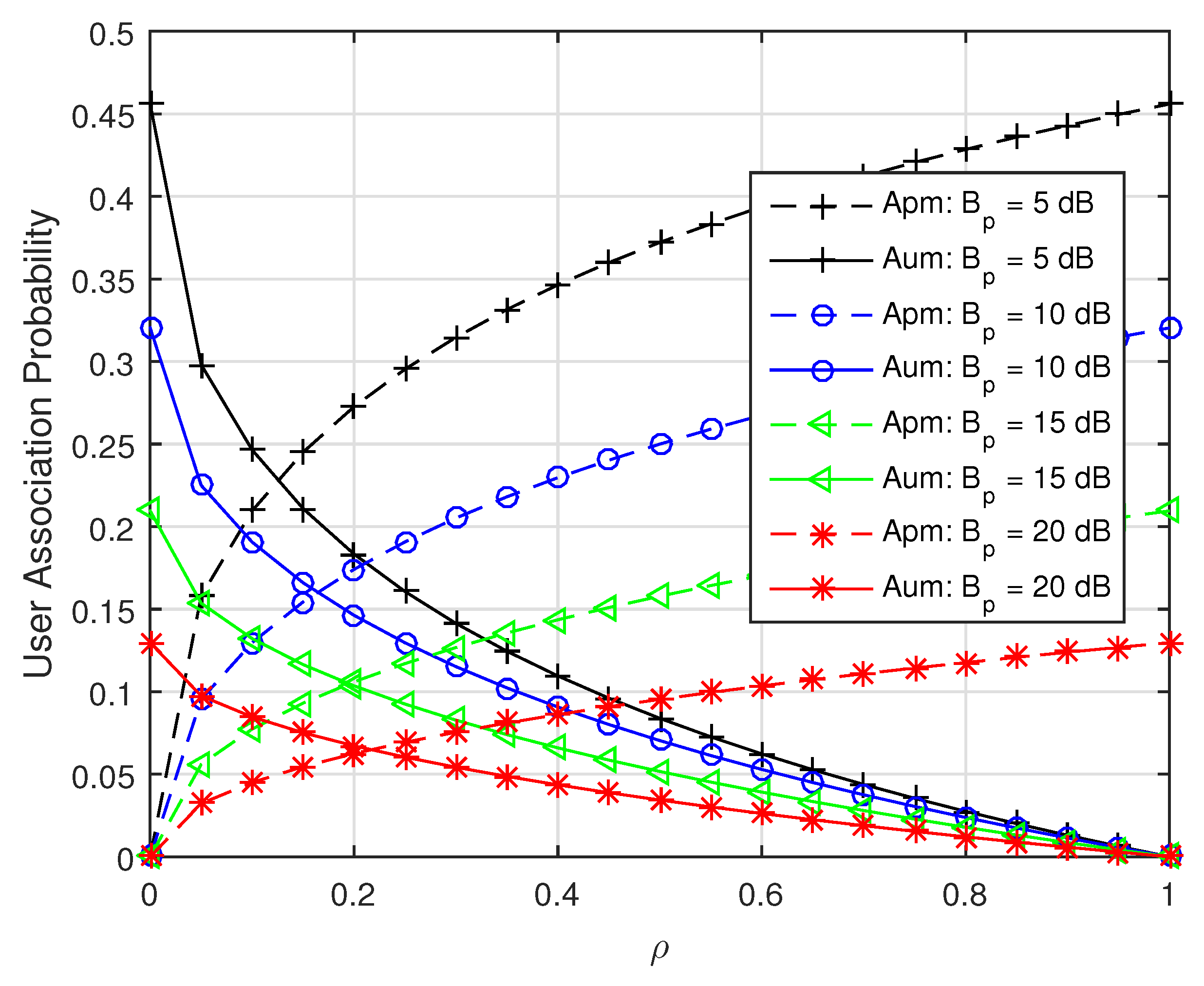
In particular, if
, then
and
, which means that the PSFs are zero power ABS. The association probabilities of USF MUEs and PSF MUEs versus
with different
are simulated according to Equation (
5) in
Figure 3. As shown in
Figure 3, with the increase of power reduction factor
, the transmission power of MBSs over PSF will increase, resulting in the association probability of USF MUEs decreasing and that of PSF MUEs increasing. It can also be found that the sum of
and
will decrease with the growth of
, because more UEs will be offloaded into pico-cells with larger
.
3.2. Distribution of Serving BS Distance
After a typical UE type is classified according to the user association strategy, the probability density function (PDF) of distance r between this typical UE and its serving BS can be obtained according to Lemma 2 as below.
Lemma 2. On the basis of user association probability deduced in Equation (5), the probability density function (PDF) of the distance r between the typical UE l and its serving BS can be derived as: 5. Joint Optimization of FeICIC Parameters and Base-Station Density
Due to the fact that MBSs are usually deployed by network operators, MBS density will change slowly and can be assumed to be constant for analysis simplification. Further simplification of the problem analysis, MBS transmit power in USF and PBS transmit power can also be assumed to be constant without considering power control. Moreover, the PSF ratio can be calculated according to Equation (
7). Hence, the network EE is mainly impacted by pico CRE bias, power reduction factor, and PBS density under different UE density, i.e., network load. As MBS density is a constant value, we can first obtain the optimal value of the ratio between PBS density and MBS density
, denoted as
, to maximize the network EE. Then the optimal PBS density
can be calculated by
. Thus, the joint optimization problem with the object of network EE maximization can be formulated as follows:
However, the network EE is nonlinear with , and , which is difficult to obtain the optimal , and at the same time with reasonable complexity. Note that the value ranges of , and are limited, which make it possible to seek out the optimal values of , and through a linear search algorithm by fixing two of these three variables, respectively. Therefore, we propose a heuristic algorithm to obtain the sub-optimal solution of the joint optimization problem in Equation (15). The proposed heuristic algorithm decomposes the original optimization problem into two sub-problems including FeICIC parameters optimization and PBS density optimization. For FeICIC parameters optimization, we first derive the approximate relation between and . Then, we get the sub-optimal values of and with given by an alternating algorithm. For PBS density optimization, the optimal value of can be obtained by a linear search method based on fixed and . Finally, we alternately solve two sub-problems to achieve globally optimal values of these variables.
5.1. Joint Optimization of Pico CRE Bias and Power Reduction Factor
In order to get the optimal values of
and
for network EE maximization, suppose that
and
are given. Thus, the pico CRE bias and power reduction factor joint optimization problem can be formulated as follow:
where
and
are the optimal values of pico CRE bias and power reduction factor, respectively. To simplify the solving process, we assume that the overall SINR of PSF MUEs is identical to that of the USF MUEs. Hence, the result of resource allocation will have a direct influence on the network
EE. In view of user fairness, the optimal network EE can be achieved when the relationship of association probabilities of PSF MUEs and USF MUEs obey the Equation (17).
Combining with Equation (
7), we can get the approximate relation of
and
as:
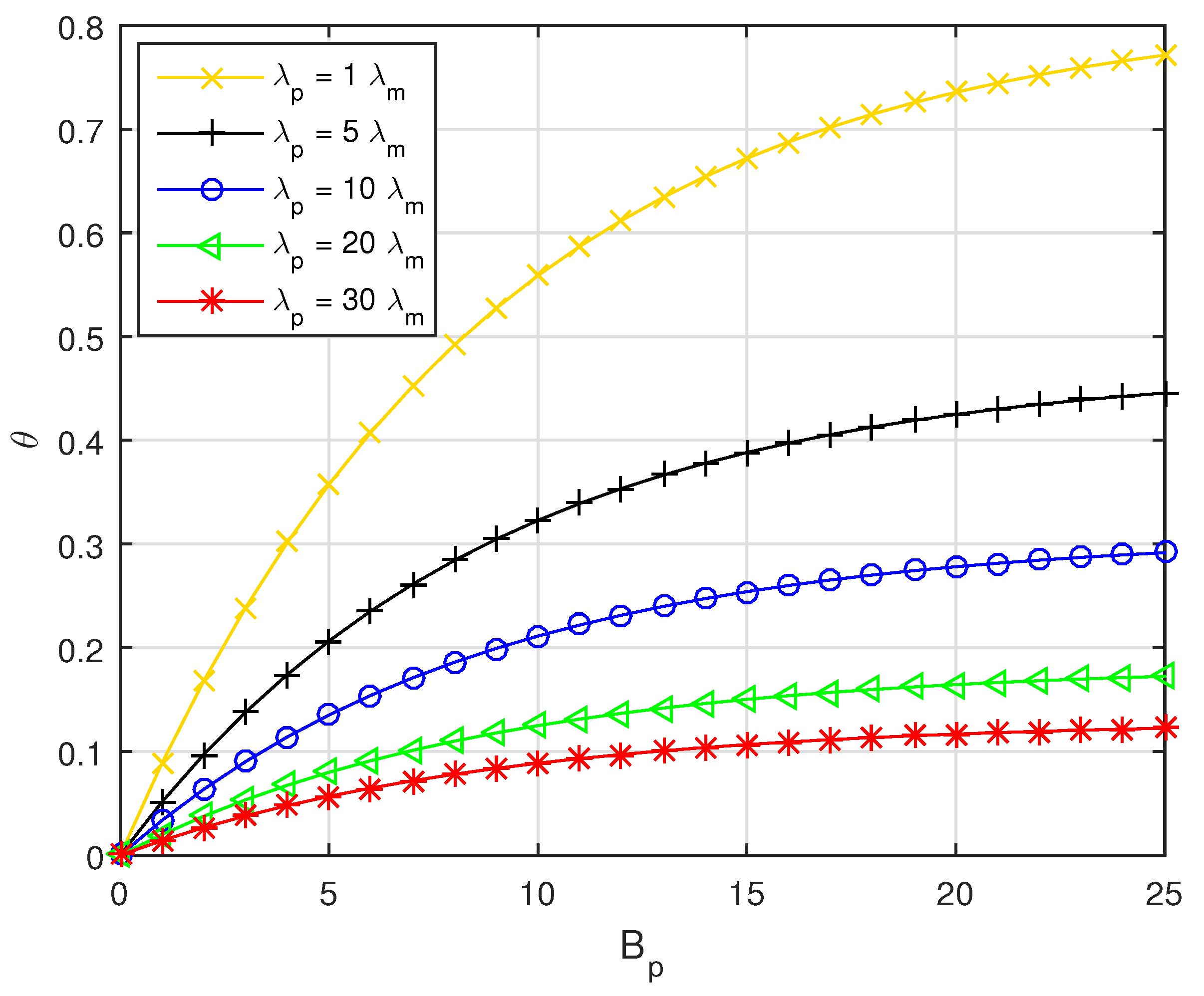
where
denotes the approximate near-optimal value of
. The relationships between
and
under different
are shown in
Figure 5. We can find that
is a strictly increasing function with respect to
at a given PBS density.
Substituting into Equation (14), we can get the near-optimal value of , denoted as by solving the following univariate problem.
Then, combining the value of with Equation (14), the near-optimal value of , denoted as can be obtained by following univariate problem.
Thus, and are obtained by an alternating algorithm, which is shown in Algorithm 1. and represent the step lengths of and , which are set to be 0.1 and 0.05, respectively. denotes the optimal value of the network EE. The main idea of this altering algorithm is to obtain the near-optimal values of pico CRE bias and power reduction factor by a two-step linear search approach on the basis of the approximate relationship between them. In line 1 of Algorithm 1, the network scenario and relative parameters are initialized. From line 2 to line 10, the optimal pico CRE bias is obtained by a linear search way on the basis of approximate relationship between pico CRE bias and power reduction factor. From line 11 to line 18, the optimal power reduction factor is calculated based on Equation (14).
| Algorithm 1: Joint pico CRE bias and power reduction factor optimization (JBPO) algorithm. |
- 1:
Initialization: Initialize the network scenario and the values , and , where . Set , , and . - 2:
whiledo - 3:
Substituting into Equation (18), the approximate near-optimal value of the power reduction factor can be obtained as . - 4:
. - 5:
Substituting and into Equation (14) with given , and , the current network energy efficiency can be obtained as: . - 6:
if then - 7:
, . - 8:
end if - 9:
. - 10:
end while - 11:
, . - 12:
whiledo - 13:
Substituting into Equation (14) with given , , and , the current network energy efficiency can be obtained as: . - 14:
if then - 15:
, . - 16:
end if - 17:
. - 18:
end while
|
5.2. Optimization of PBS Density
Similarly, suppose that
,
and
are known. Thus, the PBS density optimization problem can be formulated as follow:
Assume that the step length of is , which is set to be . Thus, the optimal PBS density can be obtained by a linear search algorithm to maximize the network EE, which is described in Algorithm 2. Line 1 of Algorithm 2 indicates the network scenario and parameters initialization. From line 2 to line 8, the optimal PBS density is acquired by a linear search method to maximize the network EE.
| Algorithm 2: Pico base stations (PBS) density optimization (PDO) algorithm. |
- 1:
Initialization: Initialize the network scenario and the values , , and , where and . Set , , and . - 2:
whiledo - 3:
Substituting into Equation (14) with given , , and , the current network energy efficiency can be obtained as: . - 4:
if then - 5:
, . - 6:
end if - 7:
. - 8:
end while
|
5.3. Joint Optimization of Pico CRE Bias, Power Reduction Factor and PBS Density
The FeICIC parameter optimization sub-problem and the PBS density optimization sub-problem are solved independently by the aforementioned optimization algorithms. Due to the fact that these variables are affected by each other, we further propose a heuristic pico CRE bias, power reduction factor and PBS density joint optimization algorithm to globally optimize network EE based on the joint pico CRE bias and power reduction factor optimization (JBPO) algorithm and PDO algorithm. The detailed procedure of our proposed heuristic algorithm is summarized in Algorithm 3. represents the positive tolerance value. is the iteration times of the algorithm. Line 1 of Algorithm 3 signifies the network scenario and parameters initialization. From line 3 to line 4, the JBPO algorithm is executed to obtain the current optimal pico CRE bias and power reduction factor at a given PBS density. From line 5 to line 6, the PDO algorithm is performed to acquire the current optimal PBS density based on the above obtained pico CRE bias and power reduction factor. From line 2 to line 9, the network EE is iteratively optimized until it cannot improve further within an arbitrary value . As a result, the optimal pico CRE bias, power reduction factor and PBS density are obtained and the network EE is maximized.
| Algorithm 3: Joint pico pico-cell range expansion (CRE) bias, power reduction factor and PBS density optimization (JBPDO) algorithm. |
- 1:
Initialization: Initialize the network scenario and the values , , , and , where , and . Set , and . - 2:
repeat - 3:
Solving the optimization problem in Equation (16), the near-optimal pico CRE bias and the near-optimal power reduction factor at given can be obtained based on the JBPO algorithm. - 4:
, . - 5:
Solving the optimization problem in Equation (21), the near-optimal PBS density at given and can be obtained based on the PDO algorithm. - 6:
, . - 7:
Substituting , and into Equation (14) with given and , the current network energy efficiency can be obtained as: . - 8:
, , , , . - 9:
until
|
5.4. Computational Complexity
The computational complexity of the JBPO algorithm can be calculated as , where and are the space sizes of the linear search for and , respectively. The computational complexity of the PDO algorithm is , where is the space size of the linear search for . Thus, the computational complexity of the JBPDO algorithm is .
Due to the fact that there does not an exist effective algorithm for solving Equation (15), we compare the computational complexity of our proposed JBPDO algorithm with that of a traversal algorithm. As for solving Equation (15), the optimal values of pico CRE bias, power reduction factor and PBS density can be obtained by a traversal way, i.e., traversal pico CRE bias, power reduction factor and PBS density optimization (TBPDO) algorithm, which refers to traversing all possible values of these three parameters to maximize the objective function in Equation (15). Thus, the computational complexity of TBPDO algorithm will be , which signifies that the computational complexity of our proposed JBPDO algorithm is reduced effectively.
As for solving the objective function in Equation (16), the optimal values of pico CRE bias and power reduction factor can also be obtained by a traversal way, i.e., traversal pico CRE bias and power reduction factor optimization (TBPO) algorithm, which refers to traversing all possible values of these two parameters to maximize the objective function in Equation (16). Indeed, TBPO algorithm consists of two nested ergodic sub-processes: (1) traversal pico CRE bias optimization (TBO) algorithm, which is executed by traversing all pico CRE bias to maximize the objective function in Equation (19) under fixed power reduction factor and PBS density; (2) traversal power reduction factor optimization (TPO) algorithm, which is executed by traversing all power reduction factor to maximize the objective function in Equation (20) under fixed pico CRE bias and PBS density. Therefore, the computational complexities of the TBO and TPO algorithms are and , respectively. As a result, the computational complexity of the TBPO algorithm will be , which is obviously higher than that of our proposed JBPO algorithm.
6. Numerical Results and Analysis
In this section, we not only provide theoretical simulation, but also verify the effectiveness of proposed heuristic algorithms by Monte Carlo simulation. In the theoretical simulation, we considerws a network coverage area within a square region of
. The deployments of PBS and MBS follow the PPP model and the typical UE is deployed in the origin. The simulation parameters used in this paper are summarized in
Table 2. We took the average results from 30 times of network implementations as Monte Carlo simulations results. In each network implementation, the locations of MBSs, PBSs and UEs were modeled as spatial PPP, respectively. Then, the network EEs was calculated for all the different combination of pico CRE bias, power reduction factor, and PBS density values within their value ranges based on wireless channel quality. Finally, the maximum network EE and the optimal pico CRE bias, power reduction factor and PBS density can be obtained by comparing the calculated network EEs under all combinations. Indeed, the results of Monte Carlo simulation, including the maximal network EE, the optimal pico CRE bias, the optimal power reduction factor and the optimal PBS density, were obtained by a traversal way in each network implementation. Meanwhile, the performances of algorithms shown in the following simulation figures were just simulated based on theoretical derived Equation (14). Therefore, Monte Carlo simulation results had the best performance and can be referred to as a baseline for valuing the performances of those algorithms.
At first, the network EE performances of the JBPO algorithm were compared with those of the TPO algorithm, TBO algorithm, theoretical simulation and Monte Carlo simulation, as shown in
Figure 6 and
Figure 7, respectively. As shown in
Figure 6, with the increase of PBS density, network EE increased accordingly. With PBS density increase, more UEs were offloaded into the coverage of low power PBSs. Then the distance between the transmitter and the receiver was shorted, resulting in network EE improvement. As shown in
Figure 7, with the increase of UE density, the curves of network EE also rose accordingly. As the UE density increased, more UEs can be offloaded into the coverage of low power PBSs by adjusting pico CRE bias and power reduction factor via network EE optimization algorithms. Then network EE can be improved. For the theoretical simulation curve, because the network EE was not optimized and just calculated according to Equation (14) with pico CRE bias and power reduction factor being set to be fixed values 5 dB and 0.25, respectively, so it had the worst performance. The TPO algorithm and the TBO algorithm optimized power reduction factor and CRE bias, respectively. Therefore, the performances of these two algorithms with one parameter optimized were better than that of the theoretical simulation. Our proposed JBPO algorithm can jointly optimize pico CRE bias and power reduction factor together. Therefore, it can further improve the network EE and match the Monte Carlo simulation results very well. Furthermore, the performance of the TPO algorithm was far less than that of the TBO algorithm, which signifies that the influence of pico CRE bias was more than that of the power reduction factor on the network EE, especially in low PBS density. In addition, in
Figure 7 the performance gap between the JBPO algorithm and theoretical simulation increases accordingly with the growth of UE density, which further indicates the importance of joint pico CRE bias and power reduction factor optimization for the heavy network load scenario.
Then, the performances of our proposed JBPO algorithm were compared with that of the TBPO algorithm in
Figure 8 and
Figure 9 from different aspects, respectively. The relationship between network EE and
with different
are shown in
Figure 8. We can see that the performance of our proposed JBPO algorithm was just slightly worse than that of the TBPO algorithm, but the computational complexity of JBPO was much lower than that of the TBPO algorithm. In addition, all curves of network EE increased first and then fell down slightly with PBS density increase, which illustrates that increasing PBS density can improve the network EE significantly within a certain network load. Nonetheless, when the PBS density exceeded a certain limit, further increasing will cause more complex interference and more power consumption, which will result in the network EE deterioration.
The relationship between network EE and
with different
are depicted in
Figure 9. Due to the curves cross with each other under different UE densities, the PBS density should be carefully adjusted according to the network load fluctuation. In addition, for a given PBS density, we can see that the network EE become greater with a higher network load. Referring to
Figure 8 and
Figure 9 together, although the network EE performance of the TBPO algorithm is just slightly better than that of the JBPO algorithm, the computational complexity of it is
, which is much higher than that of the JBPO algorithm.
Finally, the network EE performances of the JBPDO algorithm were compared with those of the PDO algorithm, JBPO algorithm with fixed
, TBPDO algorithm, and Monte Carlo simulation in
Figure 10. In the TBPDO algorithm, pico CRE bias, power reduction factor and PBS density are jointly optimized to maximize network EE by an exhaustive traversal algorithm based on Equation (14). The Monte Carlo simulation results show the maximum network EE within the value range of pico CRE bias, power reduction factor and PBS density at different network load.
As shown in
Figure 10, the proposed JBPDO algorithm can obtain better network EE than that of the JBPO algorithm since the JBPDO algorithm further optimizes the PBS density on the basis of the JBPO algorithm. Meanwhile, the accuracy and effectiveness of our proposed JBPDO algorithm are once again verified by Monte Carlo simulation results. In addition, although the network EE of the TBPDO algorithm outperforms our proposed JBPDO algorithm, the computational complexity of TBPDO algorithm is
, which is far higher than that of the JBPDO algorithm. The convergence of JBPDO algorithm is provided in
Figure 11. From
Figure 11, we can find that JBPDO algorithm can converge after three iterations. It is proved that the computational complexity of the JBPDO algorithm is much lower than that of the TBPDO algorithm and more suitable for the real-time network.


