Article

Wireless Magnetoelastic Resonance Sensors: A Critical Review

by
Craig A. Grimes
1,*,
Casey S. Mungle
1,
Kefeng Zeng
1,
Mahaveer K. Jain
1,
William R. Dreschel
2,
Maggie Paulose
2 and
Keat G. Ong
1
1
Department of Electrical Engineering & Materials Research Institute, 217 Materials Research Lab, The Pennsylvania State University, University Park, PA 16802, USA
2
SenTech Corporation, 200 Innovation Boulevard, Suite 236, State College, PA 16803, USA
*
Author to whom correspondence should be addressed.
Sensors 2002, 2(7), 294-313; https://doi.org/10.3390/s20700294
Submission received: 16 July 2002 / Accepted: 17 July 2002 / Published: 23 July 2002
(This article belongs to the Special Issue Networked Sensors and Wireless Sensor Platforms)

Abstract

:
This paper presents a comprehensive review of magnetoelastic environmental sensor technology; topics include operating physics, sensor design, and illustrative applications. Magnetoelastic sensors are made of amorphous metallic glass ribbons or wires, with a characteristic resonant frequency inversely proportional to length. The remotely detected resonant frequency of a magnetoelastic sensor shifts in response to different physical parameters including stress, pressure, temperature, flow velocity, liquid viscosity, magnetic field, and mass loading. Coating the magnetoelastic sensor with a mass changing, chemically responsive layer enables realization of chemical sensors. Magnetoelastic sensors can be remotely interrogated by magnetic, acoustic, or optical means. The sensors can be characterized in the time domain, where the resonant frequency is determined through analysis of the sensor transient response, or in the frequency domain where the resonant frequency is determined from the frequency-amplitude spectrum of the sensor.

Introduction

Magnetoelastic sensors have attracted considerable interest within the sensor community as they form an excellent sensor platform that can be used to measure a wide range of environmental parameters including pressure [1,2,3], humidity [3,4,5], temperature [5,6], liquid viscosity and density [7,8,9,10], thin-film elasticity [11], and chemicals such as carbon dioxide [12,13], ammonia [14], and pH [15]. Magnetoelastic sensors are typically made of amorphous ferromagnetic ribbons or wires, mostly iron-rich alloys such as Fe40Ni38Mo4B18 (Metglas brand 2826MB) and Fe81B13.5Si3.5C2 (Metglas 2605SC) ribbons [15] that have a high mechanical tensile strength (~1000-1700 MPa), and a low material cost allowing them to be used on a disposable basis. In addition, these Metglas ribbons have a high magnetoelastic coupling coefficient, as high as 0.98, and magnetostriction on the order of 10-5 [17,18,19]. The high magnetoelastic coupling allows efficient conversion between magnetic and elastic energies and vice versa. When excited by a time varying magnetic field, the large magnetostriction allows these materials to exhibit a pronounced magnetoelastic resonance the resonance frequency of which can be remotely detected either by magnetic, acoustic, or optical means. The environmental parameter of interest is measured by tracking the resonant frequency of the sensor.
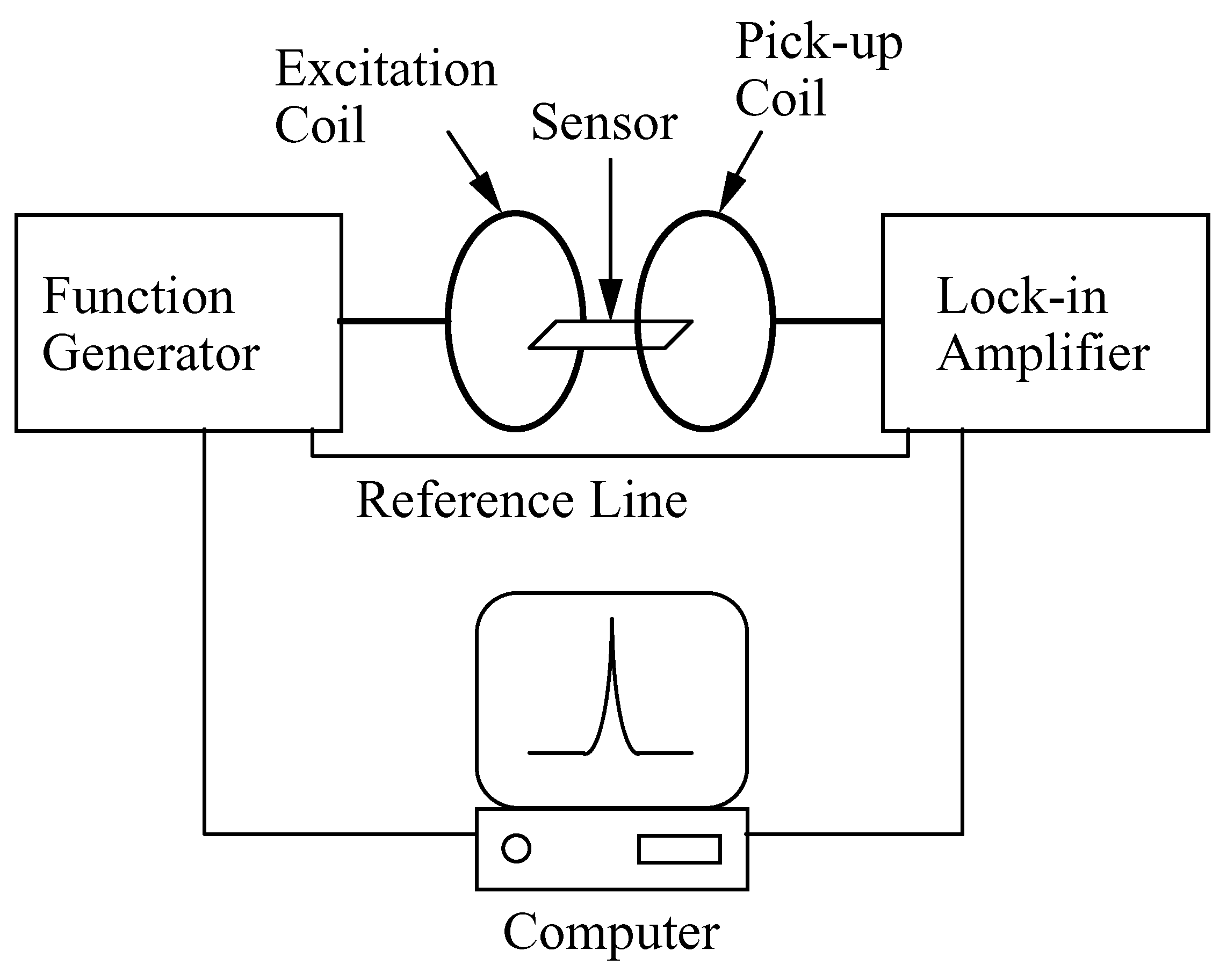
The magnetic state of the sensor, and hence its stress and temperature dependencies, are controllable by transverse-field annealing the sensor [20,
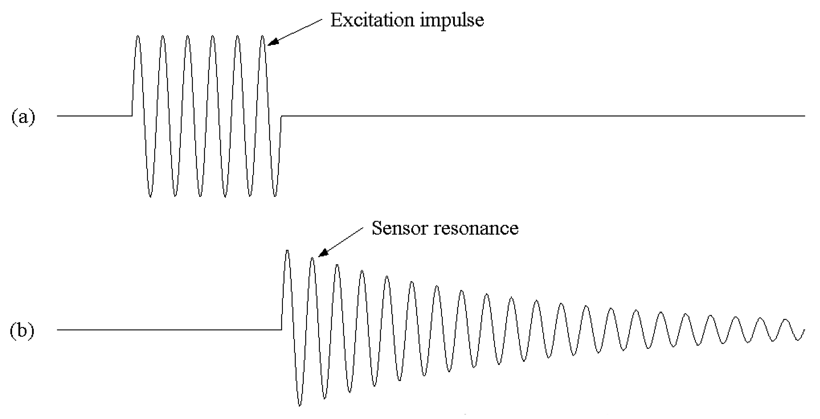
21], or changing the bias field and/or sensor aspect ratio which in turn determines the magnetic demagnetizing field of the sensor. The mechanical vibration of the magnetoelastic sensor is generated through the magnetoelastic effect by sending a time-varying magnetic signal. Through the inverse magnetoelastic effect, the vibration of the sensor in turn generates a time varying magnetic flux, which can be measured with a set of pick-up coils. The time-domain signal is then converted into the frequency domain by performing a Fast Fourier Transform (FFT), and the resonant frequency is determined [9]. The resonant frequency of the transiently excited sensor can also be determined by counting the zero crossings of the sensor response for a given time period. Alternatively, the magnetoelastic sensors can be interrogated in the frequency domain by sweeping the frequency and recording the measured amplitude each incremental frequency [22].
In addition to generating magnetic flux, the mechanical vibrations of the sensor also generate an acoustic wave that can be detected with a microphone in air or hydrophone in liquid [10]. Furthermore a laser beam can reflected from the surface of the sensor, and the response of the sensor characterized by recording the changes in the returned beam intensity. 
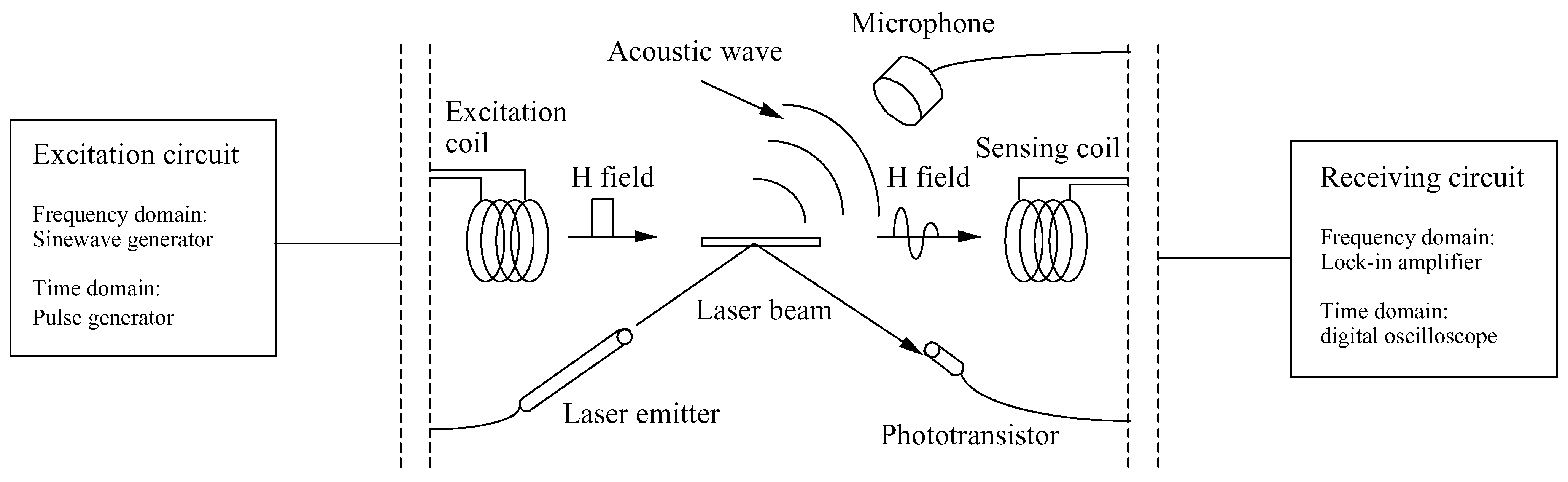
Fig. 1 illustrates the three different ways to monitor a magnetoelastic sensor: magnetically, acoustically, and optically. The magnetic detection method has the highest precision, but for a 1.0 cm long sensor has a detection range limit of approximately 30 cm. The same sensor can be detected acoustically up to approximately 2.0 m, while optical detection has been used over a 6 m range.
Figure 1. The magnetoelastic sensor is interrogated with an excitation coil producing a magnetic field impulse, and can be detected magnetically with a pickup coil, acoustically with a microphone, or optically with a laser emitter and a phototransistor.
Sensors 02 00294 g001
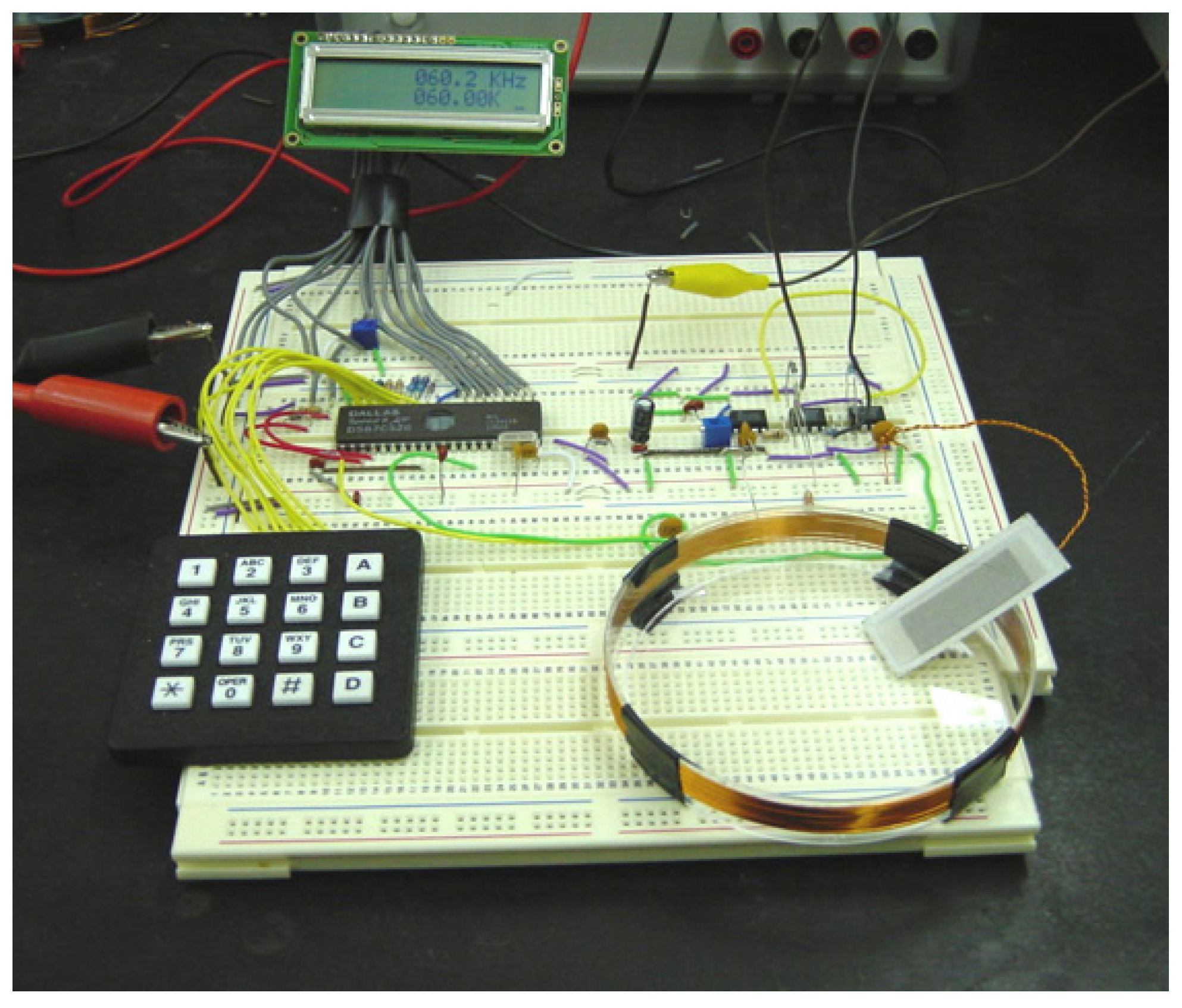
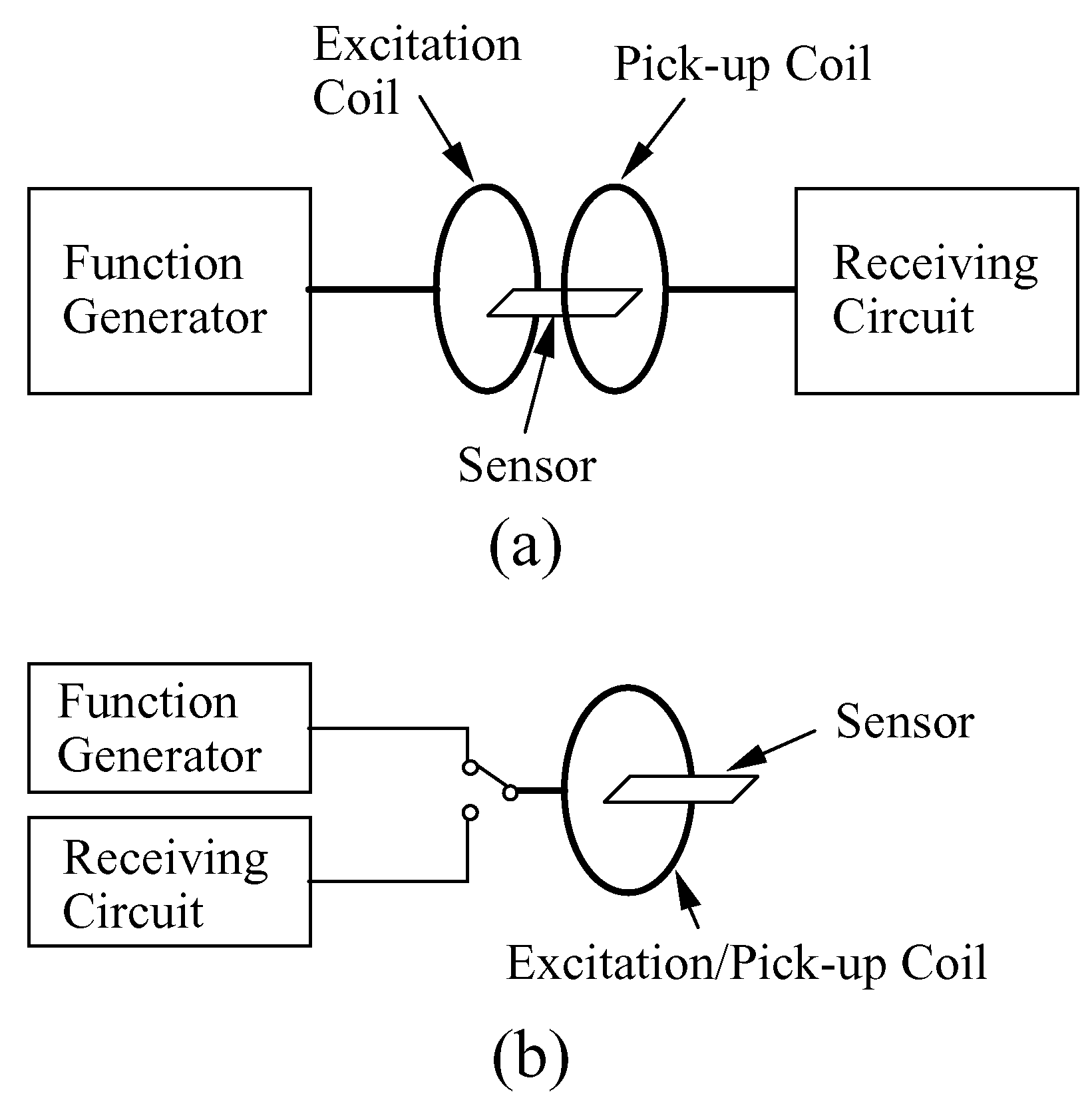
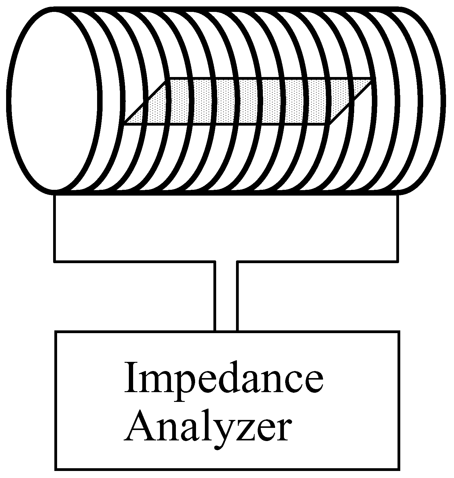
Another method of detecting the magnetoelastic sensors is to insert the sensor inside an inductor (solenoid) and measure the impedance variation in the inductor. Since the permeability of the sensor increases at the sensor resonance, the resonant frequency of the sensor can be determined by finding the frequency at which the maximum variation in the impedance of the inductor occurs. Although this method cannot detect the sensor from a distance, it requires only a single electronic instrument that measures the impedance spectrum of an inductor, i.e., an impedance analyzer.
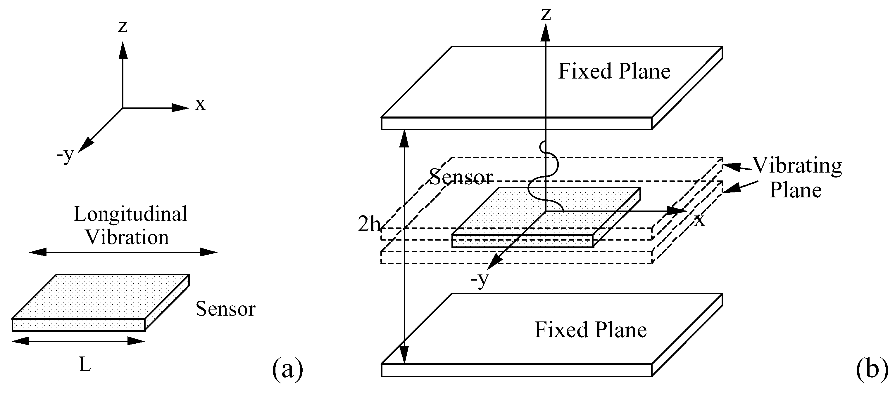
Figure 2. (a) A sensor free of external forces is modeled as a thin plate exhibiting vibration in the x-direction. (b) When immersing in a liquid, the sensor is modeled as a vibrating plate bounded by two infinite planes from a distance h and two infinite planes touching the sensor surface.
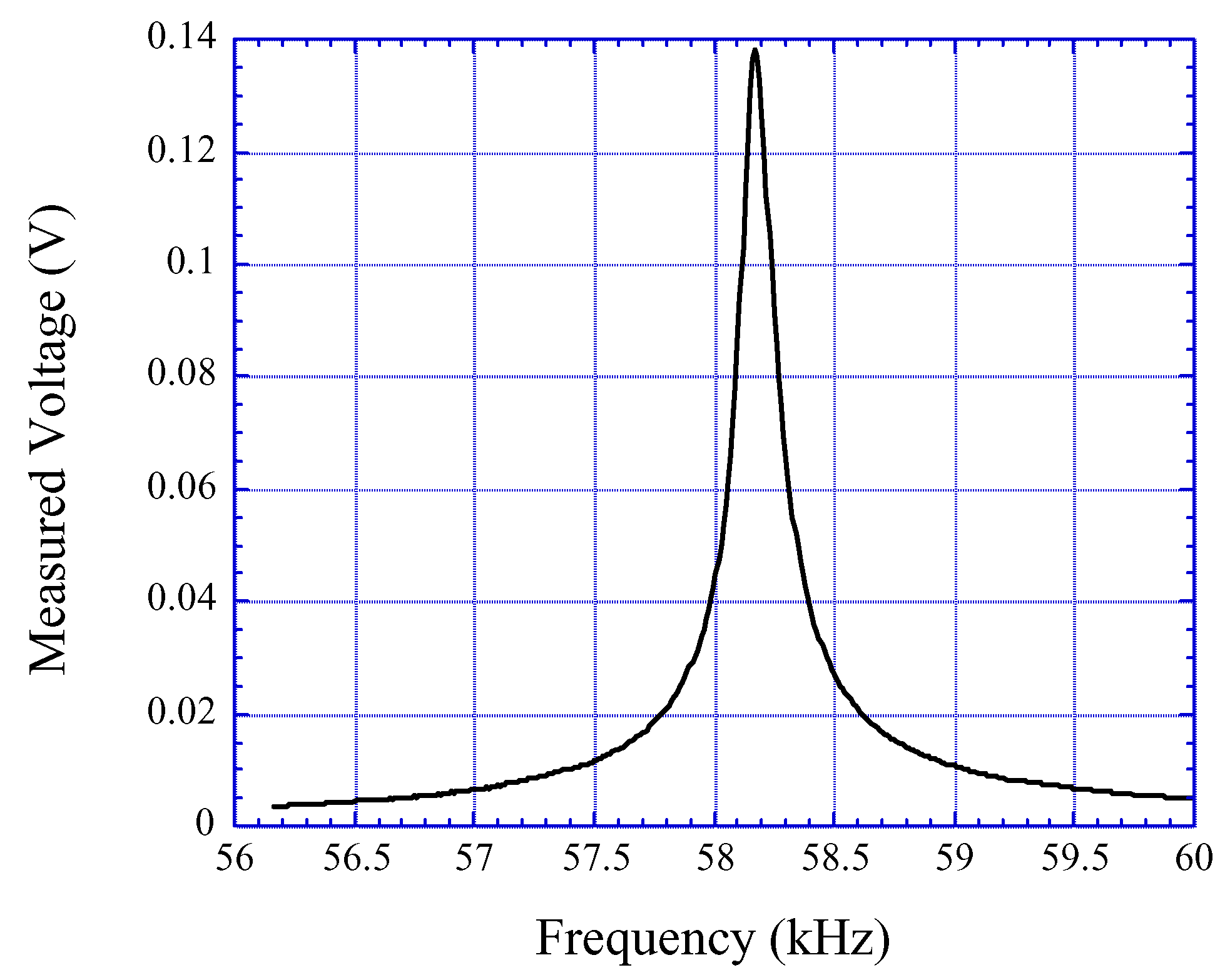
Sensors 02 00294 g002
Figure 3. The frequency response of a 4 cm × 1.3 cm × 28 µm as-cast Metglas 2826MB ribbon. The resonant frequency is the maximal of the frequency spectrum.
Sensors 02 00294 g003

Theoretical Model

The vibrating magnetoelastic sensor is modeled as a rectangular plate with its length parallel to the x-axis and excited by an x-directed ac magnetic field (see Fig. 2a), which can be described with the equation of motion as [23]:
2 u x t 2 = E s ρ s ( 1 σ 2 ) 2 2 u x x 2
where ρS is the density of the sensor, σ is the Poison’s ratio, and Es is Young’s modulus. The resonant frequency of the sensor is determined by solving Eq. (1) as:
f n = n 2 L E s ρ s ( 1 σ 2 ) n = 1 , 2 , 3
where L is the length of the ribbon. In most applications only the fundamental resonant frequency f0 (n = 1) is considered because of the higher signal amplitude and lower frequency. The fundamental resonance for a 4 cm × 1.3 cm × 28 µm Metglas 2826MB sensor ribbon, measured in air at room temperature, is shown in Fig. 3, where the resonant frequency is at the peak of the curve at 58.18 kHz.

Effect of Mass Loading the Sensor

If a coating with mass Δm is uniformly applied on the sensor surface, the density ρs in Eq. (1) can be replaced by (mS + Δm) Ad where ms is the mass of the sensor, A is the surface area, and d is the thickness of the sensor. Solving the equation of motion using the modified ρs yields a new fundamental resonant frequency fload [23]:
f l o a d = 1 2 L 1 1 + Δ m / m s A d m s E s ρ s ( 1 σ 2 ) 2 = f 0 1 1 + Δ m / m s
For mass loads small relative to the mass of the sensor the resonant frequency shift of the sensor is approximately:
Δ f = f l o a d f 0 = f 0 Δ m 2 m s

Effect of Liquid Viscosity and Density

When immersed in a viscous liquid, the resonant frequency of a vibrating sensor decreases due to the dissipative shear force created by the viscous liquid. The theoretical model for a sensor exhibiting an x-directed vibration in a viscous liquid with viscosity η and density ρl is shown in Fig. 2b, where the liquid is represented by an incompressible fluid bounded by two infinite planes on each side, one touching the sensor surface and one shifted h in the z-direction. The plane shifted h from the sensor is fixed, while the plane touching the sensor surface is vibrating in the x-direction and creating a damping force against the sensor vibration so the equation of motion in Eq. (1) becomes [8]:
2 u x t 2 = E s ρ s ( 1 σ 2 ) 2 u x x 2 2 η κ ρ s d u x t cos κ h
where κ = (1+ j)/δ with j the complex number and δ the penetration depth of the wave into the liquid given by δ = (η/πρlf)1/2. Solving Eq. (5) the fundamental resonant frequency of the sensor immersed in a viscous liquid fliquid is:
f l i q u i d 2 = E s ρ s ( 1 σ 2 ) ( 1 2 L ) 2 η f l i q u i d π δ ρ s d sinh ( 2 h / δ ) sin ( 2 h / δ ) cosh ( 2 h / δ ) cos ( 2 h / δ )
where the first term of the right hand side corresponds to the square of the resonant frequency of the sensor in an inviscid medium (identical to Eq. (2)), and the second term is the contribution of the damping force due to the liquid. In the case of highly viscous liquid, where 2 h/δ << 1, the resonant frequency shift of the sensor Δf becomes:
Δ f = f l i q u i d f 0 = 1 3 f 0 r 1 h r s h
Compared to Eq. (4), the resonant frequency shift in the viscous fluid is almost identical to that of a solid mass load except the smaller constant. This result is expected because at high viscosity the penetration depth δ is large compared to h, so the liquid layer bounded by h oscillates synchronously with the sensor just like a solid mass load. However Eq. (4) is more appropriate to describe a solid mass load because the numerical constant in Eq. (7) originates from the second term of the RHS of Eq. (6) that is only present in the liquid phase.
For a low viscosity liquid, where 2h/δ >> 1 , the resonant frequency shift becomes:
Δ f = π f 0 2 π ρ s d ( η ρ t ) 1 / 2
The resonant frequency of the sensor is proportional to the product of liquid viscosity and density. In practice, two sensors with different degrees of surface roughness are needed to separate them (see Section 4: Applications).

Effect of Coating Elasticity

Eq. (4) describes the relationship between the resonant frequency and a uniformly applied mass load. However, it does not consider the elastic stress in the mass load, applying only to a mass load of translational oscillation, not one of contraction and expansion. To consider the effect of coating elasticity on the sensor resonant frequency, the effective Young’s modulus Eeff and density ρeff of a uniformly coated sensor are expressed as [24]:
E e f f = α c E c + α s E s
ρ e f f = α c ρ c + α s ρ s
where Ec and Es are the Young’s modulus of the coating and the sensor, respectively, and ρc and ρs are the density of the coating and sensor, respectively, and αc and αs are the fractional thicknesses of the coating and the sensor, respectively. Substituting Eqs. (9) and (10) into Eq. (2), and assuming the Poisson ratio σ is close to zero, the fundamental resonant frequency of the coated sensor fcoat is:
f c o a t = 1 2 L α c E c + α s E s α c ρ c + α s ρ s
The ratio of the resonant frequency of the coated sensor to a bare sensor is:
f c o a t f 0 = α c E c + α s E s α c ρ c + α s ρ s ρ s E s = 1 + α c ( E c / E s 1 ) 1 + α c ( ρ c / ρ s 1 )
Eq. (12) can be simplified by relating αc to the total mass mt and the sensor mass ms as [24]:
α c = m t / m s 1 m t / m s 1 + ρ c / ρ s
and becomes:
f c o a t f 0 = ( 1 β 2 ) 2 m t m c + β 2 = m t m c + ( 1 β 2 ) 2 m t m c
where β is:
β = E c / ρ c E s / ρ s
Eq. (14) can be used to determine the elasticity of a coating provided that the density and mass of the coating, and the elasticity, density and mass of the sensor are known.

Effect of Temperature and Applied Field

Eq. (2) describes the resonant frequency as a function of mechanical properties. To extend the model to include the change in elasticity with applied field, i.e. the ΔE effect, we first note ΔE is expressed as [25]:
Δ E E s E s E M E s = 9 κ s 2 ( T ) E s ( T ) H 2 M s ( T ) H k σ 3 ( T )
where T is the temperature, λs is the magnetostriction, H is the applied field, Ms is the saturation magnetization, H is the anisotropy field when the sensor is under a longitudinal stress σ, EM is the modulus of elasticity at constant magnetization, and Es is the modulus of elasticity at field H. Substituting Eq. (16) into Eq. (2) and including the temperature dependence of the different variables, the resonant frequency f0 is expressed as [26]:
f 0 ( T , H ) = 1 2 L ( T ) E s ( T ) ρ s ( T ) ( 1 + 9 κ s 2 ( T ) E s ( T ) H 2 M s ( T ) H k σ 3 ( T ) ) 1 / 2
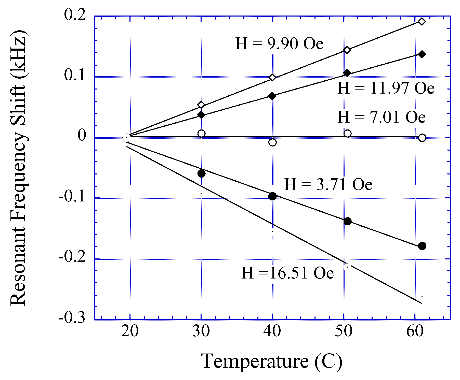
The consequence of Eq. (17) is that an applied dc biasing field of appropriate magnitude can be used to cancel the temperature dependence of the sensor.

Detection Systems

Time-Domain Measurement

With time domain characterization the sensor is excited by a magnetic field impulse, comprised of a sinusoidal wavetrain, as shown in Fig. 4a. Current passed through a coil is used to generate the magnetic excitation field. The sensor response (see Fig. 4b), an exponentially decaying sinusoidal signal (i.e. the ‘ring down’), can be detected with another coil, or with the same coil if a switch is used to isolate the excitation and receiving circuits as illustrated in Fig. 5. The resonant frequency of the sensor can be determined from the ring down response using two different techniques: frequency counting and FFT. Using the FFT algorithm, the time-domain response of the sensor is converted into frequency-domain, and the resonant frequency is determined by finding the peak of the frequency- domain spectrum. The frequency counting technique determines the resonant frequency of the sensor by counting the numbers of oscillations of the ring-down signal at a given time period. Generally, the frequency counting technique is simpler and requires less complicated circuitry, however it cannot categorize the resonance quality, or sharpness, of the sensor. Figure 6 shows a simple frequency counting circuit based upon a Dallas Semiconductor Corporation DS87C520 microcontroller that can be used to characterize magnetoelastic sensors in the range of 30 kHz to 200 kHz.
Figure 4. (a) The excitation signal is a series of sinusoidal bursts. (b) The sensor response is an exponentially decaying sinewave, or the ring-down.
Sensors 02 00294 g004
Figure 5. Time domain detection system. (a) In the two-coil configuration, the excitation coil is used to generate the excitation pulse and the pick-up coil receives the sensor response. (b) Only one coil is needed for excitation and reception if an electronic switch is used to isolate the excitation circuit and receiving circuit.
Sensors 02 00294 g005
Figure 6. The electronics of a time-domain system using only one coil for excitation and receiving. The resonant frequency of the sensor is determined via frequency counting using a Dallas Semiconductor Corporation DS87C520 microcontroller.
Sensors 02 00294 g006

Frequency-Domain Measurement

The frequency-domain system requires an excitation coil and a pick-up (detection) coil. The excitation coil is connected to a function generator to generate a fixed-frequency steady state signal, and the pick-up coil measures the sensor response at that frequency. The frequency of the steady state signal is gradually increased, maintaining steady state operation, and the sensor response at a desired frequency range is measured. The resonant frequency of the sensor is determined by finding the frequency where the amplitude of the sensor is greatest.
Figure 7. The frequency-domain detection system. A function generator is used to excite the sensor, and the response of the sensor is recorded via a lock-in amplifier.
Sensors 02 00294 g007
Figure 7 shows a frequency-domain detection system. A function generator is used to generate the steady state signal. The received sensor response is sent to a lock-in amplifier to be amplified and measured. A reference line is connected from the function generator to the lock-in amplifier so the amplifier can precisely measure the signal at the excitation frequency. A computer is used to control the operation as well as collect and process data.

Impedance De-tuning Method

The magnetoelastic sensor can also be detected with an inductive solenoid. The sensor is inserted inside the solenoid as shown in Fig. 8, and the impedance of the solenoid is measured as a function of frequency. Since the permeability of the sensor increases significantly at resonance, a sharp peak will occur in the solenoid’s impedance spectrum at the resonant frequency of the sensor.
Figure 8. The magnetoelastic sensor can be detected by placing inside a solenoid and measuring the impedance variation of the solenoid.
Sensors 02 00294 g008

Applications

Temperature Monitoring

As indicated by Eq. (17), the resonant frequency shift of a magnetoelastic sensor can be positive or negative, large or small, depending upon the mechanical and magnetic properties of the sensor and the magnitude of the applied field. For a temperature sensor, an appropriate field H can be applied to the ribbon to yield an optimum temperature sensitivity; for other sensor applications, e.g. the measurement of fluid flow velocity in a changing temperature environment, the value of H can be chosen so the sensor has no temperature dependency. The temperature dependency of a 3 × 1.3 cm × 28 µm 2826MB Metglas sensor is plotted in Fig. 9 as a function of varying H field amplitudes. From the plot, the maximum positive temperature dependency happens at H = 9.9 Oe, maximum negative temperature dependency at H =16.51 Oe, and zero-temperature dependency can be achieved at H = 7.01 Oe.

Humidity Monitoring

A magnetoelastic humidity sensor was built by coating a layer of titanium dioxide (TiO2) on a 4 × 1.3 cm Metglas 2826MB ribbon [4]. As the humidity increases, water vapor is absorbed into the TiO2 layer, increasing the effective mass on the sensor. Fig. 10 shows the increase in humidity decreases the resonant frequency. In addition to TiO2, alumina (Al2O3) was also used as a coating for humidity monitoring [5], and the results are similar to that of TiO2.
Figure 9. The resonant frequency shifts of a magnetoelastic sensor verses temperature and bias field H. The highest positive temperature dependency happens at H = 9.9 Oe, highest negative temperature dependency at H =16.51 Oe, and zero-temperature dependency at H = 7.01 Oe.
Sensors 02 00294 g009
Figure 10. The resonant frequency shift of a TiO2-coated humidity sensor as a function of humidity concentration; the TiO2 coating changes mass in response to humidity level, in turn shifting the resonant frequency of the sensor.
Sensors 02 00294 g010

Pressure Monitoring

A flat sensor is insensitive to pressure because it exhibits longitudinal vibration that has a limited interaction with gas molecules at the surface. To increase the sensitivity, an out-of-plane vertical vibration is created on the sensor by bending the sensor. The resonant frequency shift of a bent sensor as a function of pressure can be expressed as [1]:
Δ f [ 1 3 σ 2 1 σ m g u k B T d ρ s ] p
where p is the pressure, d is the thickness of the sensor, u is the maximum vibration amplitude, T is the temperature, kB is the Boltzmann’s constant, and mg is the mass of gas. Eq. (18) indicates the resonant frequency decreases with increasing pressure. This conclusion is consistent with the experimental results in Fig. 11, where the resonant frequency of a 4 × 1.3 cm 2826MB Metglas reduces linearly with pressure, and the pressure dependence increases with curvature of the sensor.
Figure 11. The resonant frequency decreases as the atmospheric pressure increases; r denotes the radius of curvature of the curved sensor.
Sensors 02 00294 g011

Flow Rate Monitoring

A magnetoelastic sensor can also be used to measure liquid flow rates since the flowing liquid creates a damping force, proportional to the flow rate, on the sensor surface and causes a shift in the sensor resonant frequency [27]. A magnetoelastic fluid-flow sensor was fabricated using a 4 × 1.3 cm 28 µm 2826MB Metglas ribbon immersed in a water pipe with its length placed parallel to the liquid flow direction. The experimental results, plotted in Fig. 12, show the resonant frequency decreases with increasing fluid flow velocity while in the laminar regime, and then shifts upwards after reaching the turbulent flow regime.
Figure 12. The resonant frequency decreases quadratically at laminar liquid flow (<115 cm/s), and increases again when the liquid switches from laminar to turbulent flow.
Sensors 02 00294 g012

Measurement of Liquid Viscosity and Density

Eq. (8) indicates the resonant frequency of the sensor decreases as a function of the square root of the product of the liquid viscosity η and density ρl. In the equation η and ρl are inseparable, hence it is not possible to measure η and ρl with a uniformly smooth sensor. However, due to surface roughness, liquid is trapped by the sensor surface and acts as a mass load. To compensate for the liquid density and surface roughness dependent mass loading, an additional term is added in Eq. (8) [7]:
Δ f = π f 0 2 π ρ s d ( η ρ l ) 1 / 2 ρ l Δ V f 0 2 m s
where ΔV is the volume of liquid trapped by the surface roughness of the sensor, and ms is the mass of the sensor. From Eq. (19) the liquid density and viscosity can be separated by using two sensors with different surface roughnesses, indicated by subscript 1 and 2, with the difference in the resonant frequencies of the two sensors given by:
Δ f 2 Δ f 1 = ρ ( Δ V 1 Δ V 2 ) f 0 2 M
Using Eq. (20), the density and viscosity of the glycerin-water mixture was simultaneously determined [7] with two 30 mm × 3 mm × 28 µm 2826MB Metglas ribbons, one uncoated, and one coated with TiO2 on both sides giving the two sensors different degrees of surface roughness.

Measurement of Thin-Film Elasticity

Using Eq. (14), the elasticity of a thin-film coating can be determined by monitoring the shifts in the resonant frequency of a coated sensor with respect to a bare sensor. To determine the elasticity of the coating, the mass and resonant frequency of the uncoated ribbon is first measured. A uniform coating is then applied and the resonant frequency and mass are determined. The process is repeated N times until sufficient data points are collected. The value of β can then determined by applying a least-square fit on the collected data using Eq. (14) as [24]:
ρ = i = 1 N ( ( f t i f 0 ) 2 m 0 m t i ) ( 1 m o m t i ) i = 1 N ( 1 m o m t i ) 2
The parameters Es, ρs, and ρc are measured before the experiment. The Young’s modulus of the material of interest Ec is determined by substituting the calculated β into Eq. (15). Fig. 13 plots the frequency shift of a silver-coated sensor as a function of coating mass. The data points were fitted with Eq. (21) and Es of silver is determined as 74.8 GN/m2, a difference of only 1.6% from the theoretical value. Experiments for calculating the Young’s moduli of aluminum, polyurethane paint, and acrylic paint have also been conducted with errors of less than 2% with theoretical values [24].
Figure 13. The relative resonant frequency of a magnetoelastic sensor decreases linearly with increasing mass of silver coating. A least square-fit (dashed line) is used to calculate the Young’s modulus of the silver.
Sensors 02 00294 g013

Chemical and Gas Sensing

By applying a mass-changing chemically responsive layer magnetoelastic sensors have been used to monitor chemical analyte concentrations including glucose [28], carbon dioxide (CO2) [13], ammonia (NH3) [14], and pH [15]. Generally, the mass change for these chemically responsive layers is small, so the resonant frequency shift is linear as described in Eq. (5). For example, Fig. 14 shows that the resonant frequency of the CO2 sensor, based on an acrylamide and isooctylacrylate coating, decreases linearly with the percentage CO2. Fig. 14 also shows the sensitivity of the sensor increases with the coating thickness until 20 µm, where the mass load is too large for the sensor to resonate. Table 1 lists various magnetoelastic chemical (liquid and gas) sensors that have been built and tested.
Figure 14. A magnetoelastic CO2 sensor, where the slope of the resonant frequency shift increases with the coating thickness.
Sensors 02 00294 g014
Table 1. Magnetoelastic sensors have been used to monitor CO2, NH3, pH, and glucose based upon the mass change of chemically responsive layers.
SensorChemically Responsive LayerSensitivityRangeStabilityRef
CO2Acrylamide + isooctylacrylate-5.6 Hz/vol%0 – 50 vol%Stable13
NH3Poly(acrylic acid-co- isooctylacrylate)-14 Hz/log(vol%)0 – 100 vol%Stable11
PHAcrylic acid (20 mol%) + iso-octyl acrylate(80 mod%)-333 Hz/pH5.5 – 8.5 pHStable14
GlucosePVA and a co-polymermade of DMAA, BMA, DMAPAA, and MAAPBA-13 Hz / (mg/L)0 – 100 mg/LDissolves after 3 - 4 high/low cycles28

Magnetoelastic Sensor Arrays

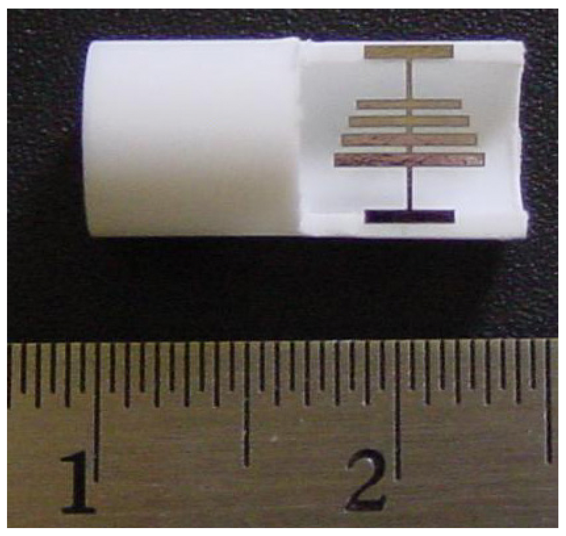
A magnetoelastic sensor array can be constructed by placing sensors of different length (with different resonant frequencies) in parallel as shown in 
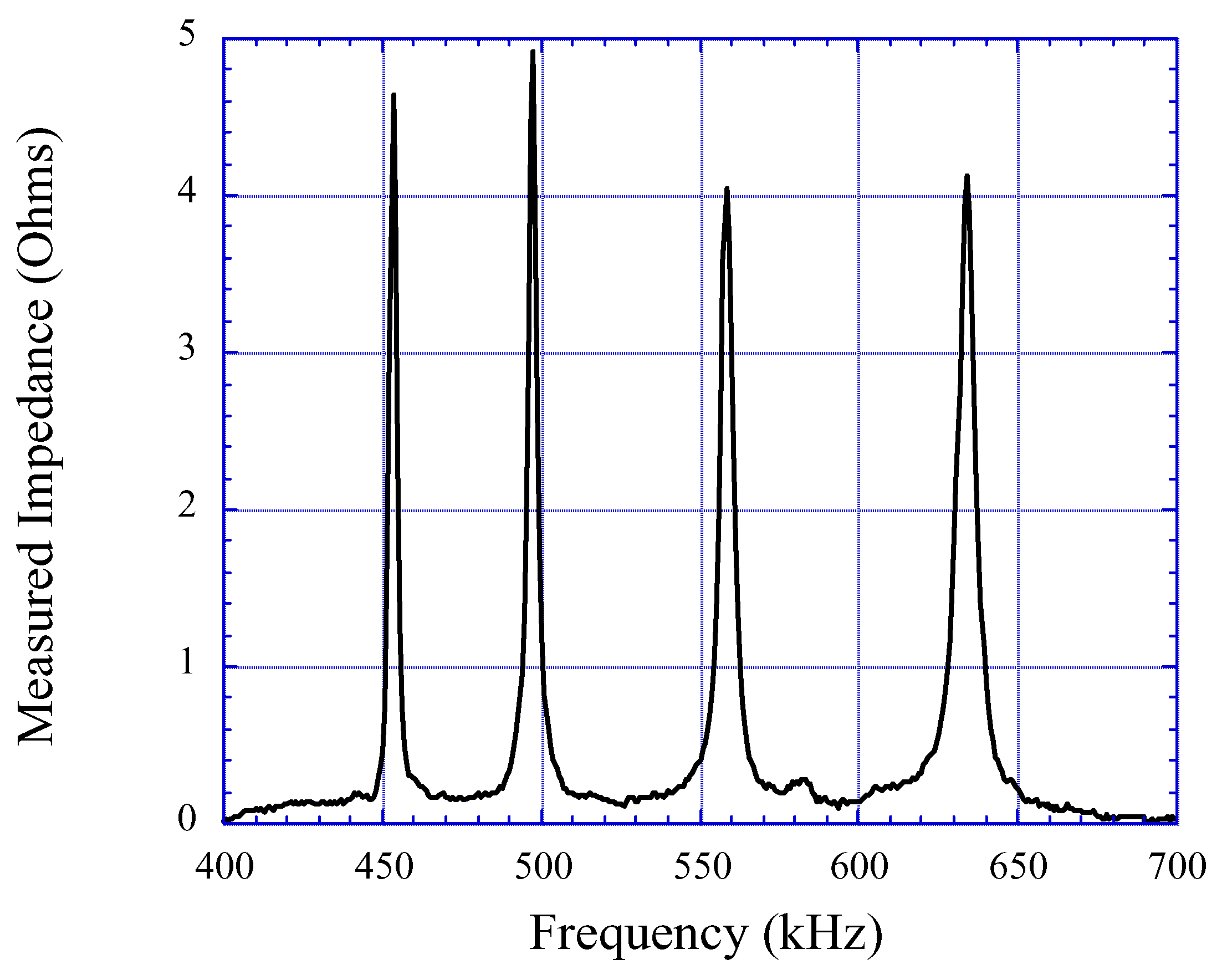
Fig. 15. Since the magnetoelastic sensors operate via mechanical vibrations, they can be monitored simultaneously with minimum interference. As shown in Fig. 16, the resonance of the four sensor elements can be distinctively measured. The array elements can be designed, or biased, to enable simultaneous multi-parameter sensing. For example, adjacent placement of a magnetically hard biasing strip of sufficient field strength will cancel the effect of temperature, enabling pressure measurement in a changing temperature environment. Alternatively, a perfectly flat sensor will not respond to changes in pressure, enabling temperature to be measured in a changing pressure environment. The effect of fluid flow velocity can be countered by placing the sensors within a porous protective shell, etc.
Figure 15. A magnetoelastic sensor array consisting of four sensor elements (the four horizontal strips at the center) mounted on a tube at its support tabs (the top and bottom strips). The major scale is in cm.
Sensors 02 00294 g015
Figure 16. The frequency response of the four-element sensor array measured by inserting the sensor array into a solenoid. The impedance of the solenoid is eliminated with a background subtraction.
Sensors 02 00294 g016

Optimizing Sensor Performance

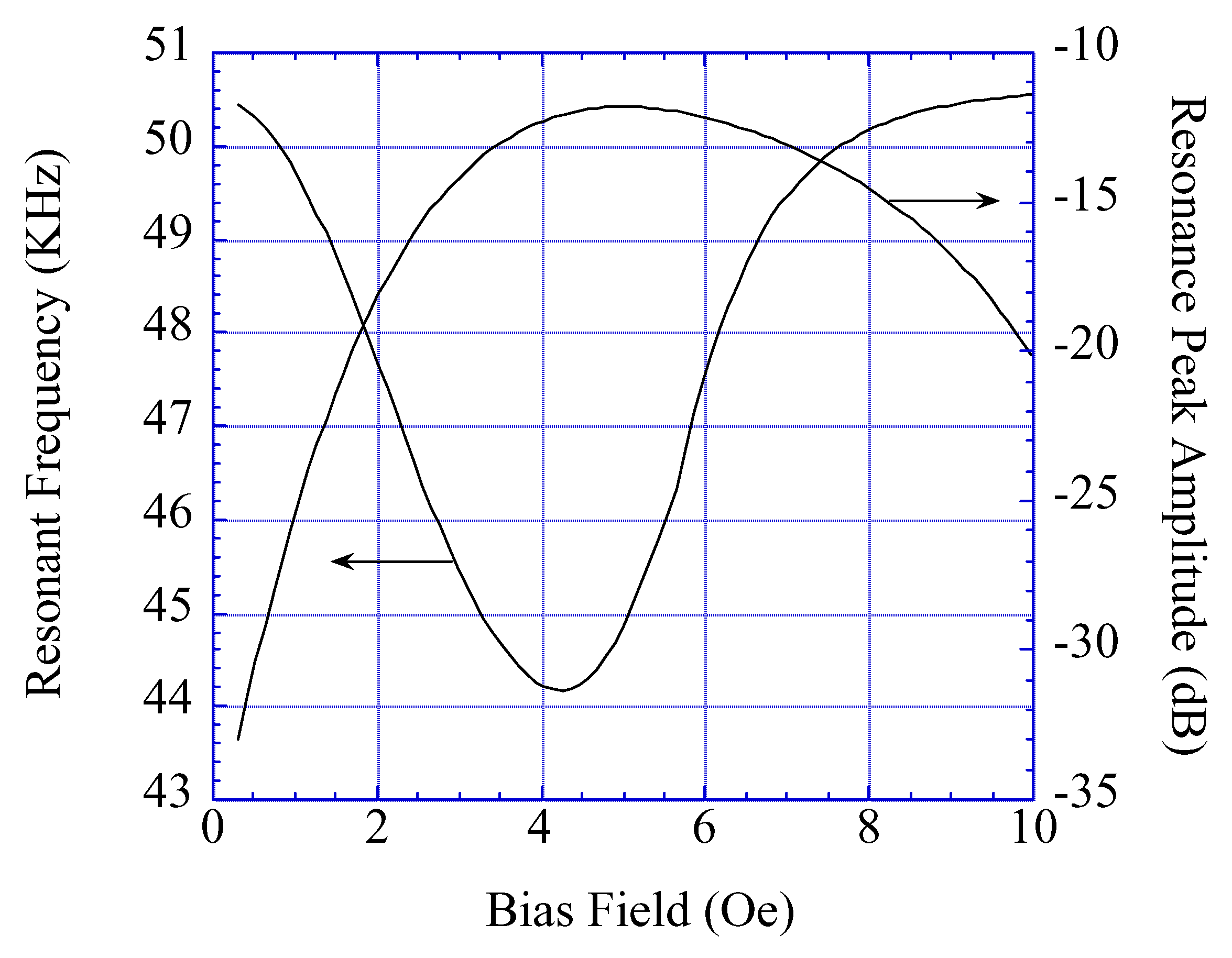
Fig. 17 shows the resonant frequency shift of a magnetoelastic sensor as a function of bias field amplitude. The shift in the resonant frequency and change in measured amplitude is due to the change of elasticity Es, the so-called ΔE effect, due to the changing bias field. Fig. 17 shows there is an optimal bias field where sensor amplitude is maximum, which corresponds to the anisotropy field of the sensor Hk [25].
Figure 17. The resonant frequency and amplitude of a magnetoelastic sensor varies with applied field amplitude H due to changing elasticity (ΔE effect).
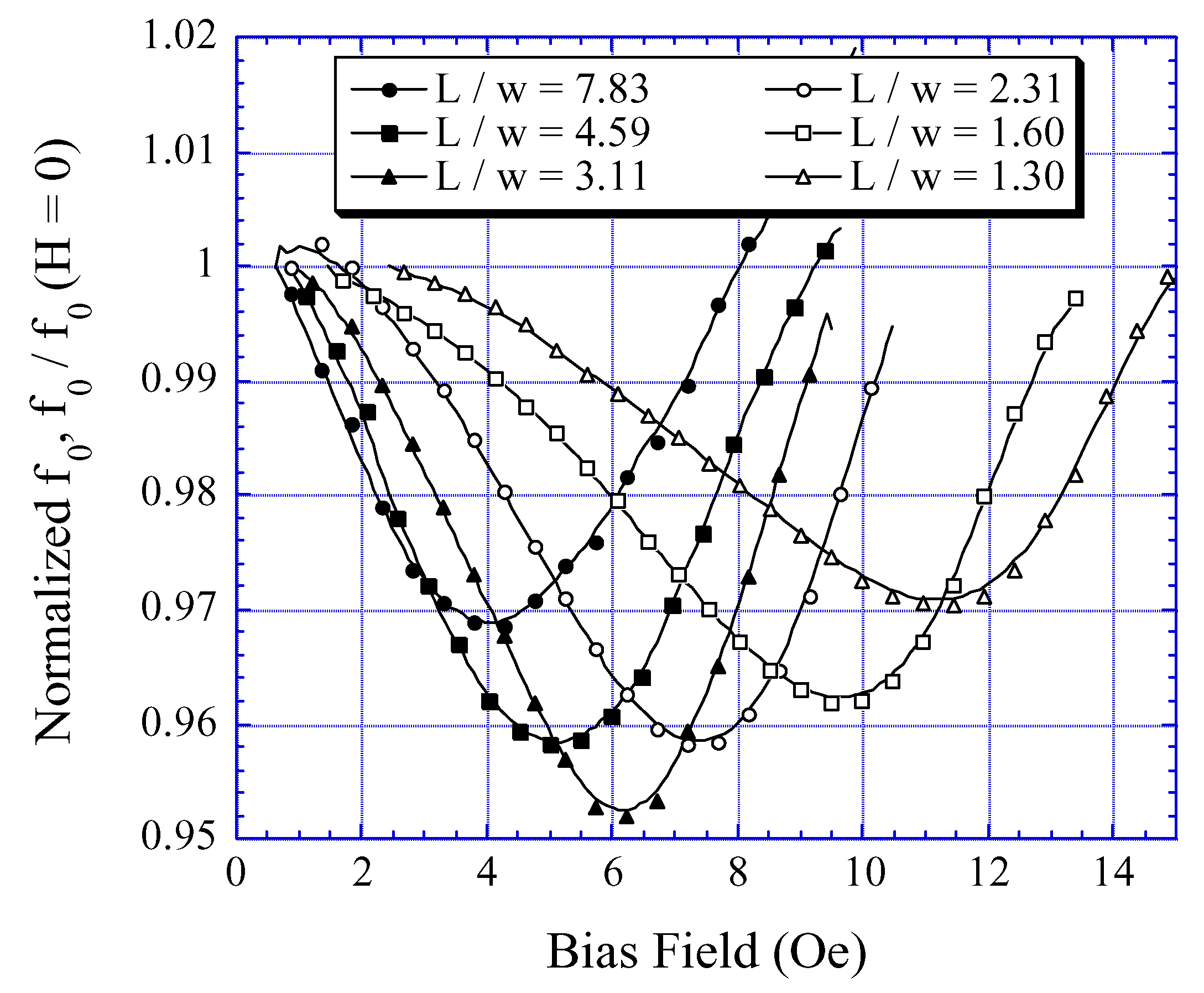
Sensors 02 00294 g017
Figure 18. The applied bias field required for the sensor to exhibit maximum ΔE effect increases with decreasing sensor length to width ratio.
Sensors 02 00294 g018
Although the anisotropy field Hk does not change with sensor length, the applied H field has to be increased when the length of the sensor is reduced to compensate for the demagnetizing field and to maintain the internal field, Hi, at Hk. The internal field Hi is given as:
Hi = HMD
where M is the magnetization and D is the demagnetizing factor. Fig. 18 plots the resonant frequency as a function of the sensor length to width ratio and H. As can be seen from Fig. 18, a higher bias field is required for the sensor to exhibit maximum ΔE effect as the aspect ratio of the sensor decreases. The applied field for maximum 
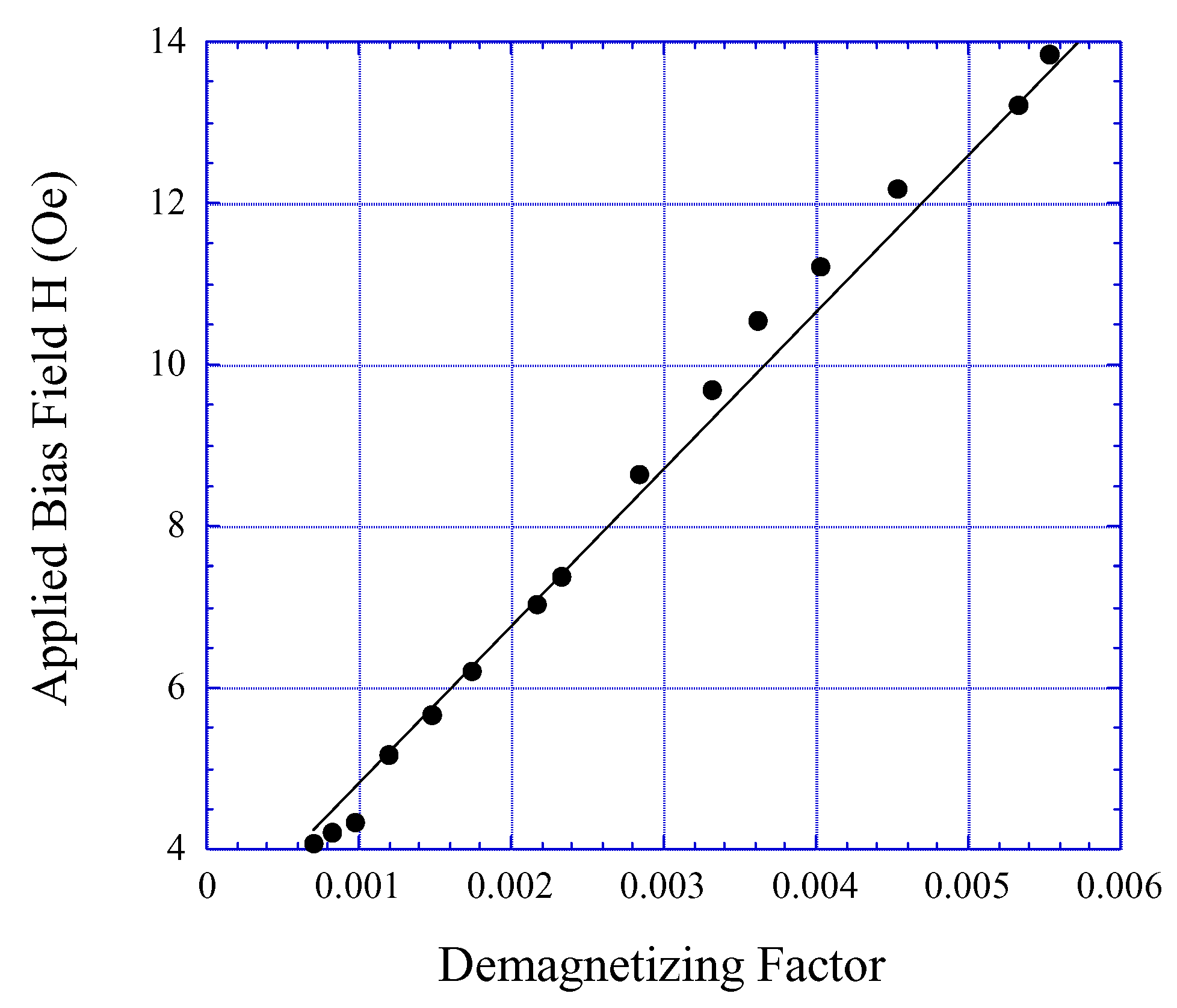
ΔE effect linearly increases with demagnetizing factor D as illustrated in Fig. 19.
Figure 19. The optimal bias field increases linearly with the demagnetizing factor of the sensor.
Sensors 02 00294 g019
Figure 20. Transverse-field annealing of the magnetoelastic sensor increases the ΔE effect and decreases the anisotropy field Hk.
Sensors 02 00294 g020
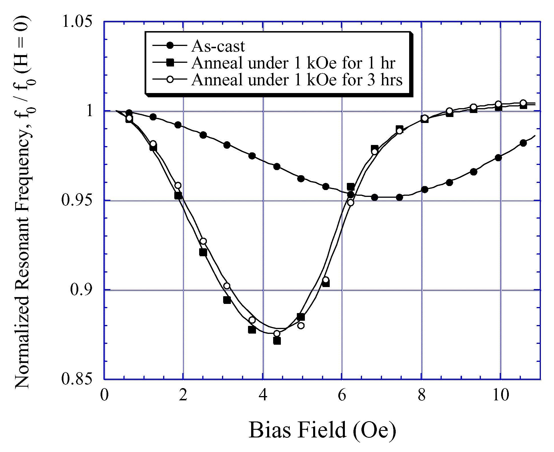
Another way to increase the sensor performance and the magnitude of the ΔE effect is by annealing the sensor while exposed to a transverse magnetic field [21,22,29,30]. Fig. 20 shows the bias-field dependent resonant frequency of an as-cast 4 × 1.3 cm × 28 µm 2826MB ribbon, and the same ribbon after a 1 kOe transverse field anneal at 350°C for 1 hr and 3 hr. As can be seen, the magnitude of the ΔE effect of the transverse-field annealed sensors is improved by more than 150%, while Hk is reduced by 30%.

Conclusions

The operational principles and applications of magnetoelastic sensors are presented. Magnetoelastic sensors are amorphous ferromagnetic ribbons that exhibit a magneto-mechanical resonance when excited by a time varying magnetic field. Magnetoelastic sensors have successfully been used for stress, pressure, liquid viscosity and density, fluid flow velocity, elasticity, and temperature monitoring. Chemical sensors based on the magnetoelastic sensor platform have been fabricated by combining the magnetoelastic sensors with mass changing, chemically responsive layers (both polymeric and metal oxides).
Theoretical models have been developed to understand the behavior of the sensor under different operating conditions. For small mass loads the resonant frequency of the sensor is found to linearly decrease. For uniformly applied coatings the shift in resonant frequency is proportional to the difference in the speed of sound between the coating and sensor; a coating with a speed of sound identical to that in the sensor material will not induce a shift in resonant frequency. The resonant frequency of a sensor immersed in liquid is dependent upon the product of the liquid viscosity and density; two sensors with different surface roughnesses can be used to separate the two effects. To measure atmospheric pressure, the sensor is bent so it exhibits out-of-plane vibrations, increasing by several orders of magnitude the surface area able to interact with the ambient atmosphere.
For optimal performance, the magnetoelastic sensor is set to operate at the point where it exhibits highest ΔE effect. The optimal operating point for the sensor is set by changing the bias field or the dimension of the sensor. Generally, a higher bias field is needed to set the sensor at the optimal operating point when the length of the sensor decreases. This is due to the demagnetizing field of the sensor, which increases with decreasing sensor aspect ratio. Annealing the sensor under transverse fields also increases the performance of the sensor by increasing the ΔE effect, which will increase the magnetoelastic coupling, and reducing the anisotropy field. The bias field can be used to counteract mechanical properties, enabling a temperature independent response with proper biasing field amplitude. By proper selection of differently designed magnetoelastic elements a sensor array can be made able to simultaneously measurement multiple environmental parameters.

Acknowledgments

Support of this work by NSF through grant ECS-0196494 and NASA through grant NAG-1-01036 is gratefully acknowledged.

References

  1. Kouzoudis, D.; Grimes, C. A. The frequency response of magnetoelastic sensors to stress and atmospheric pressure. Smart. Mater. Struct. 2000, 8, 885–889. [Google Scholar] [CrossRef]
  2. Grimes, C. A.; Stoyanov, P. G.; Kouzoudis, D.; Ong, K. G. Remote query pressure measurement using magnetoelastic sensors. Rev. Sci. Instrum. 1999, 70(12), 4711–4714. [Google Scholar] [CrossRef]
  3. Grimes, C. A.; Kouzoudis, D. Remote query measurement of pressure, fluid-flow velocity, and humidity using magnetoelastic thick-film sensors. Sens. Actuators 2000, 84, 205–212. [Google Scholar] [CrossRef]
  4. Grimes, C. A.; Kouzoudis, D.; Dickey, E. C.; Qian, D.; Anderson, M. A.; Shahidian, R.; Lindsey, M.; Green, L. Magnetoelastic sensors in combination with nanometer-scale honeycombed thin film ceramic TiO2 for remote query measurement of humidity. J Appl. Phys. 2000, 87(9), 5341–5343. [Google Scholar]
  5. Jain, M. K.; Schmidt, S.; Ong, K. G.; Mungle, C.; Grimes, C. A. Magnetoacoustic remote query temperature and humidity sensors. Smart Mater. Struct. 2000, 9, 502–510. [Google Scholar]
  6. Jain, M. K.; Cai, Q. Y.; Grimes, C. A. A wireless micro-sensor for simultaneous measurement of pH, temperature, and pressure. Smart Mater. Struct. 2001, 10, 347–353. [Google Scholar]
  7. Grimes, C. A.; Kouzoudis, D.; Mungle, C. Simultaneous measurement of liquid density and viscosity using remote query magnetoelastic sensors. Rev. Sci. Instrum. 2000, 71(10), 3822–3824. [Google Scholar] [CrossRef]
  8. Stoyanov, P. G.; Grimes, C. A. A remote query magnetostrictive viscosity sensor. Sens. Actuators 2000, 80, 8–14. [Google Scholar] [CrossRef]
  9. Loiselle, K. T.; Grimes, C. A. Viscosity measurements of viscous liquids using magnetoelastic thick-film sensors. Rev. Sci. Instrum. 2000, 71(3), 1441–1446. [Google Scholar] [CrossRef]
  10. Jain, M. K.; Schmidt, S.; Grimes, C. A. Magneto-acoustic sensors for measurement of liquid temperature, viscosity, and density. Appl. Acoustic 2001, 62, 1001–1011. [Google Scholar] [CrossRef]
  11. Ong, K. G.; Jain, M. K.; Mungle, C.; Schmidt, S.; Grimes, C. A. Magnetism-based sensors (Invited paper). Proceedings of SPIE 2001, 4467, 158–172. [Google Scholar]
  12. Kouzoudis, D.; Grimes, C. A. Remote query fluid-flow velocity measurement using magnetoelastic sensors. J Appl. Phys. 2000, 87(9), 6301–6303. [Google Scholar]
  13. Cai, Q. Y.; Cammers-Goodwin, A.; Grimes, C. A. A wireless remote query magnetoelastic CO2 sensor. J Environ. Monit. 2000, 2, 556–560. [Google Scholar] [CrossRef]
  14. Cai, Q. Y.; Jain, M. K.; Grimes, C. A. A wireless, remote query ammonia sensor. Sens. Actuators B 2000, 77, 614–619. [Google Scholar] [CrossRef]
  15. Cai, Q. Y.; Grimes, C. A. A remote query magnetoelastic pH sensor. Sens. Actuators B 2000, 71, 112–117. [Google Scholar] [CrossRef]
  16. Honeywell, 101 Columbia Road, Morristown, NJ 07962 USA. http://www.honeywell.com.
  17. Hernando, A.; Vazquez, M.; Barandiaran, M. Metallic glasses and sensing applications. J Phys. E: Sci. Instrum. 1988, 21, 1129–1139. [Google Scholar] [CrossRef]
  18. Modzelewski, C.; Savage, H. T.; Kabacoff, L. T.; Clark, A. E. Magnetomechanical coupling and permeability in transversely annealed Metglas 2605 alloys. IEEE Trans. Magn. 1981, MAG-17(6), 2837–2839. [Google Scholar] [CrossRef]
  19. O’Handley, R. C. Modern Magnetic Materials: Principles and Applications; John Wiley & Sons, Inc.: New York, 2000. [Google Scholar]
  20. Brouha, M.; van der Borst, J. The effect of annealing conditions on the magnetomechanical properties of Fe-B-Si amorphous ribbons. J Appl. Phys. 1979, 50(11), 7594–7596. [Google Scholar]
  21. Soyka, V.; Kraus, L.; Zaveta, K.; Jurek, K. Magnetoelastic properties of stress/field annealed Fe80Cr2B14Si14 amorphous alloy. J Magn. Magn. Mater. 1999, 196–197, 262–263. [Google Scholar] [CrossRef]
  22. Grimes, C. A.; Ong, K. G.; Loiselle, K.; Stoyanov, P. G.; Kouzoudis, D.; Liu, Y.; Tong, C.; Tefiku, F. Magnetoelastic sensors for remote query environmental monitoring. Smart Mater. Struct. 1999, 8, 639–646. [Google Scholar]
  23. Grimes, C. A.; Cai, Q.; Ong, K. G.; Loiselle, K. Environmental monitoring using magnetoelastic sensors. Proc. SPIE 2000, 4097, 123–133. [Google Scholar]
  24. Schmidt, S.; Grimes, C. A. Characterization of nano-dimensional thin-film elastic moduli using magnetoelastic sensors. Sens. Actuators A 2001, 94(3), 189–196. [Google Scholar] [CrossRef]
  25. Livingston, J. D. Magnetomechanical properties of amorphous metals. Phys. Stat. Sol. A 1982, 70, 591–596. [Google Scholar] [CrossRef]
  26. Mungle, C. Optical detection of magnetoelastic sensors and the variable temperature response of the resonant frequency. Dissertation University of Kentucky 2001. [Google Scholar]
  27. Kouzoudis, D.; Grimes, C. A. Remote query fluid-flow velocity measurement using magnetoelastic thick-film sensor (invited). J Appl. Phys. 2000, 87(9), 6301–6303. [Google Scholar]
  28. Grimes, C. A.; Stoyanov, P.; Liu, Y.; Tong, C.; Ong, K. G.; Loiselle, K.; Shaw, M.; Doherty, S.; Seitz, W. A magnetostatic-coupling based remote query sensor for environmental monitoring. J Phys. D: Appl. Phys. 1999, 32, 1329–1335. [Google Scholar]
  29. Price, M. H.; Overshott, K. J. The vibration of initial permeability of amorphous ribbons with frequency and annealing conditions. IEEE Trans. Magn. 1983, MAG-19(5), 1931–1933. [Google Scholar] [CrossRef]
  30. Anderson, P., III. Magnetomechanical coupling ΔE effect and permeability in FeSiB and FeNiMoB alloys. J Appl. Phys. 1982, 53(11), 8101–8103. [Google Scholar] [CrossRef]
  • Sample Availability: Available from the authors.

