1. Introduction
The Barkhausen effect specifically refers to the phenomenon in which the magnetic flux of a magnetized material changes discontinuously due to magnetic domain inversion during magnetization [
1]. As an important nondestructive testing (NDT) method, the magnetic Barkhausen noise (MBN) signal is sensitive to the changes in many material properties and has many applications in the fields of material stress and hardness detection [
2,
3,
4,
5], metal fatigue state analysis [
6], metal microstructure transformation, and grain size measurement [
7].
As the direct carrier for excitation and reception of MBN signal, the characteristics of sensor determine the quality of the MBN detection result. We adopted a self-developed MBN sensor with high spatial resolution. In detail, the MBN sensor is mainly composed of an excitation device and an MBN signal receiving device. The excitation part is a U-shaped yoke composed of a plurality of overlapping silicon steel sheets, and the excitation coil is composed of a multi-hit coil wound around the U-shaped yoke, which are used to excite an alternating magnetic field. The receiving device uses a magnetic core-wound coil receiver, which is generally placed between the two yokes of the U-shaped yoke while keeping perpendicular to the test piece for measurement. In order to improve the spatial resolution and measurement stability of the sensor, we add a layer shielding shell with high permeability and conductivity to the outside of the receiver, limiting the effective signal receiving area of the MBN sensor to a relatively small local area. In addition, we increased the number of turns for the pickup coil, so as to achieve the purpose of getting good sensitivity and frequency response characteristics in a lower frequency range.
Intensity changes in an MBN signal with material state transformation are usually reflected and described by the representative parameters calculated in time-frequency (TF) domain such as the amplitude, energy, root mean square (RMS), waveform full width at half maximum (FWHM), envelope, peak time, threshold, and power spectrum [
3,
4,
5,
8,
9,
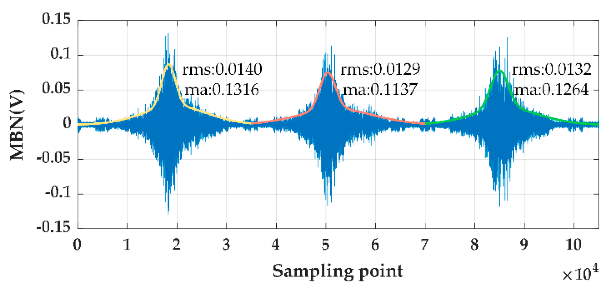
10]. However, affected by the microscopic magnetic anisotropy of the material itself, measurement performance, and experimental magnetization parameters (such as magnetization intensity and frequency, excitation waveform), the MBN has an obvious stochastic nature and the application of more automatic signals processing procedures used for extraction, selection, and fusion of signal features containing critical and distinctive information about the material properties are urgently required.
Figure 1 provides an intuitive understanding of the stochastic characteristic of the MBN signal, in which distinctive differences can be drawn from different wave packets of MBN signals. According to the relevant literatures, multiple signal processing methods have been applied to get more representative information of MBN signal. Magalas [
11] introduced wavelet transform into MBN signal analysis; then, Miesawicz et al. [
12] further expanded the study. Luo et al. [
13] applied the auto-regressive modeling method to obtain a single-sided power spectrum (also called a PSD or an AR spectrum), which is a near-deterministic expression of the MBN signal. In [
14,
15,
16], Hilbert–Huang Transform and Short-Time Fourier Transform (STFT) are used to analyze the joint TF representation and properties of MBN signal. In addition, wide new features are also proposed. Vashista et al. [
17] proposed two parameters of “count” and “event” of MBN signal; on this basis, Hang [
10] used a genetic algorithm (GA) for appropriate threshold selection. Su et al. [
4] performed first- and second-order derivation on the AR spectrum and manually extracted some peaks from it as new features. Li et al. [
5] adopted a modified slow feature analysis (m-SFA) to enrich the content of PSD by fusing the AR spectrum with different orders. There are many types of features, which can be roughly divided into energy feature, statistical feature, and shape feature, and great differences may manifest for different features used in different applications. When a variety of new features continue to be extracted, the problem of feature explosion arises, and various dimensionality reduction methods are needed to decrease the redundancy of features such as PCA [
4,
9], FCA [
9], and forward-selection combined with cross-validation [
18]. It is complex work.
Although researchers have proposed many excellent methods for MBN signal processing so that features can have good linearity and low dispersion, reducing the influence of the random characteristics of MBN signal on the detection or prediction results. There are three problems that must be considered in these methods. The first one is that many new features are not reproducible on cycling. In some cases, once the materials, experimental equipment and methods are changed, the new features may be useless and are not always superior to the conventional features, lacking in universality and versatility. The second, definite explanations and definitions about the laws of the stochastic nature of MBN signal haven’t been made. Thirdly, due to the particularity of different features, we cannot use uniform standards to analyze, define, and classify the performance of features, making the features analysis and selection complicated.
Summarizing the works of others, we aim to make further study on the internal quality of the random characteristics of MBN signal and transform it into the accurate quantification of signal uncertainty and sensitivity, to solve the three problems above. For data uncertainty measurement, the most commonly used are probabilistic methods based on data statistics such as Monte Carlo method and Bayesian analysis [
19]. Among them, Bayesian analysis has a great advantage in making full use of historical information and continuously integrating new data to learn the accurate probability distribution of data when the sample is unbalanced and short. In Bayesian learning, clarifying the role of prior and likelihood information in Bayesian inference of large models is necessary. Likelihood reflects the amount of data to some degree and Prior represents how certain the researcher is about model parameters being estimated [
20]. In [
21,
22], the discussion has also been given out. It can be concluded that, when accurate informed priors are specified, the amount of theory (via the prior) incorporated into the model estimation process increases. Specifically, with strong and accurate priors, less data would likely be needed to properly estimate parameter values. In contrast, more data would be needed in cases where no theory was incorporated. Helton et al. [
23] carried out eigenvalue uncertainty analysis on nuclear data using a survey of sampling-based statistical methods and discussed the influence of data uncertainty caused by the data amount and the degree of dispersion on the uncertainty of model prediction. In [
21], Sarah et al. used Bayesian statistics for mixture uncertainty modeling, illustrating the importance of a prior sensitivity analysis, and discussing how to interpret results that fluctuate with different prior settings.
Based on these analyses, in a complex system, two distinct sources of uncertainty can be considered: feature(observation) uncertainty and model uncertainty [
24,
25]. In this paper, we specify that the stochastic quality of MBN signal is characterized as features uncertainty. Model uncertainty arises from the inability to specify an exact value for a parameter that is assumed to have a constant value in the respective investigation, and accounting for uncertainty in model parameter estimations makes the model robust to alleviate overfitting without a need for regularization [
26]. Specifically, Bayes by Backprop modeled on variational inference was proposed to measure the weight uncertainty in a neural network [
27]. Likewise, we try to model the parameters uncertainty of a multivariable linear regression (MLR) model, in which the posterior distribution of parameters can be inferred by Bayes’ theorem without using complicated variational inference. Moreover, output uncertainty analysis can be used to study how the sensitivity propagates from the uncertainty changes of input features and model parameters to the model predictions, which is called the prediction uncertainty. In other words, uncertain outputs can be treated as functions of uncertainty analysis of inputs and model parameters. In general, we aim to quantify uncertainty in the input features of MBN signals, uncertainty in the parameters of the learning model, and uncertainty in the output predictions produced by the input and parameters characterized as probability distribution based on the modeling of sensitivity and uncertainty. This has the potential to improve modeling flexibility and accuracy. The benefit of using Bayesian learning in our study is that they offer a unified and consistent set of tools for uncertainty and sensitivity measurements for modeling, inference, prediction, and model selection [
28,
29]. The methods given in this article include the following:
First, feature uncertainty is modeled by reparameterization sampling. Specifically, we perform interval sensitivity analysis based on the confidence intervals of the feature distribution. A certain interval value is selected as the measurement index of signal uncertainty by applying reparameterization sampling of feature matrices. When the uncertainty is maintained, a more robust feature group is reconstructed by uniformly quantizing the features extracted from the same signal wave packet. Then, model uncertainty is measured by BLR. For BLR, prior distribution (prior) selection and training are of great importance. Incorporating informed priors into the estimation process can improve convergence and prediction accuracy. Due to a lack of prior knowledge, we propose an effective method in this paper to assign model parameters more reasonable priors by calculating the gradient descent of the Kullback–Leibler (KL) divergence between the prior distribution and posterior distribution. In addition, prediction uncertainty is characterized as the statistical mean and variance of prediction for each fatigue state and is used as the evaluation index of the results of interval sensitivity analysis and prior sensitivity analysis. Prediction uncertainty is applied to measure the sensitivity of observation uncertainty and model uncertainty.
The rest of this paper is arranged as follows:
Section 2 introduces the experimental setup and measurements. The main algorithm derivation and modeling process are illustrated in
Section 3.
Section 4 presents the experiment results and related analysis. Finally, the research in this paper is summarized and concluded in
Section 5.
2. Experimental Setup and Measurements
The experimental system mainly consists of a low-frequency fatigue test machine (Shimadzu (China) Co., Ltd. Beijing, China) the MBN measurement instrument and the fatigue test piece. The measurement system was self-built and included a signal generator Handyscope hs3 (TiePie engineering, Amazing Tech Co., Ltd, Shenzhen, China), power amplifier Newton LPA05A (Newtons4th Ltd, Beijing Miko-Xinye Electronics Technology Co., Ltd. Beijing, China), preamplifier Stanford SR560 (Stanford Research Systems), self-developed current collector and magnetic Barkhausen signal sensor, and computer. The testing specimens are manufactured from carburized 20R steel (American: AISI/SAE, 1020, Britain: BS, IC22), whose chemical composition is shown in
Table 1, and the full-size and shape were designed according to National standard. In the process of specimen preparation, the surface is ground to Ra1.6 roughness, then annealed at a high temperature of 550 °C for 6 h, and then the surface oxide scale with diluted hydrochloric acid is removed. The maximum magnetic field strength in the test sample is 99 A/m, and the saturation induction intensity of the sample is 1.5–2T, and the magnetic field intensity must be greater than 10,000 A/m when it reaches saturation. Then, tensile tests were carried out on specimens before the fatigue test. The lower yield strengths of the two specimens were 297 MPa and 301 MPa, and the corresponding tensile strengths were 443 MPa and 448 MPa. Through trial and error, 345 MPa was selected as the maximum tensile stress for the fatigue test. The test stress ratio was 0, and the stress change was in the form of a sinusoid wave with a frequency of 15 Hz. The MBN signal and the magnetic characteristic signal excited at the center of the specimen were measured after a certain cycle period.
The sensor used in the experiment is a magnetic core wound coil type shielded sensor designed based on non-destructive testing technology, which aims to solve the problem of low spatial resolution of the current coil wound sensor. The coil is made of manganese-zinc ferrite, and the noise of the coil itself without the specimen is consistent with the noise level of the system without the sensor. In the process of measurement, we use a rubber band to fix the sensor probe on the surface of the material. The tension of the rubber band is very small and can be ignored. The yoke of sensor contacts the specimen, and the pick-up is located between the two yokes and not in contact with specimen, so it is not affected by head pressure. The configuration block diagram of the experimental system is shown in
Figure 2; during the experiment, the software on the computer controls the signal generator to emit a sinusoidal signal at the specified frequency. The sinusoidal signal is amplified by the power amplifier and then sent to the excitation coil through the current collector so that the alternating magnetic field is generated in the tested component and the MBN signal is excited.
Moreover, considering that the received signals are susceptible to the excitation signal and external factors, the measured MBN signals were filtered by a bandpass filter to remove the low-frequency and high-frequency interference signals. The detailed excitation and acquisition parameter settings are listed in
Table 2. In order to better observe and compare the random characteristics of the different wave packets, we set a long signal acquisition channel to ensure that a sufficient number of signal wave packets (150) with the same sampling points (35,000) could be split from the continuous signal. Meanwhile, a dataset with enough samples was created for prediction.
The whole life cycle of ferromagnetic materials consists of the loading time from loading free to break. Due to the dispersiveness of fatigue, in order to reduce the experimental error, the same fatigue experiment and MBN signal measurement were carried out on three specimens taken from the same base material. The fatigue life cycle of three specimens measured in the experiment were 42,712 times, 54,643 times and 47,762 times, respectively. To explore the MBN signal across the whole life cycle of the ferromagnetic materials, the MBN signal was collected every 1000 cycles until the materials broke. To avoid the influence of experimental measurement errors, we randomly selected MBN signals under 12 measuring moments that corresponded to certain fatigue loading times for analysis, and we regarded each loading time as a different fatigue state.
3. Modeling for the Uncertainty
Given a dataset, the choice of model and parametrization of the regression function are of the utmost importance. Our aim is to establish an accurate model using probability uncertainty and sensitivity analysis that does this reasonably well. This paper focuses on uncertainty modeling, including the uncertainty analysis of features, model parameters, and predictions. In any practical setting, we have access to only a finite, potentially large, amount of data for selecting the model class and the corresponding parameters. Given that this finite amount of training data does not cover all possible scenarios, we may want to describe the remaining parameter uncertainty to obtain a measure of confidence of the model’s prediction at test time. The smaller the training set is, the more important the uncertainty modeling.
Consistent modeling of uncertainty provides model predictions with confidence bounds. The overall implementation process of this paper is illustrated in
Figure 3 and includes two main parts. The first part summarizes the modeling process of observation uncertainty, in which signal preprocessing and feature extraction are carried out and the uncertainties in the signal are characterized as multiple normal distributions of the features. The second part is the measurement of model parameter uncertainties for prior setting and posterior training.
Given a set of training example pairs
, we aim to find a function
that maps input
to corresponding function values
. For this dataset,
and
denote the size of the feature matrices characterized as
. Each element in the sample space
refers to an example with
features. We index the examples and features as
and
, respectively. We assume that a linear model is used for prediction. The functional relationship between
and
is given by
where
are the model parameters (regression coefficients) that we are about to measure and
is an independent random variable that describes the measurement noise, which can also be called zero-mean Gaussian-distributed noise.
3.1. Observation Uncertainty Analysis Based on Reparameterization Sampling
In this section, the method of modeling observation uncertainty using probability distributions is given. The stochastic nature of MBN signal in this paper can be understood as signal instability, which affects the robustness and characterization of features. That is, the same feature extracted from different wave packets has different values. Based on these considerations, we aim to reconstruct the features to varying reparameterization degrees (manifested as confidence intervals of a Gaussian distribution) from the probability perspective to infer and define the uncertainty in the MBN signals.
In observation uncertainty analysis of any multi-to-one response system using sampling methods, three steps are mainly considered: (1) Calculate the mean vector and covariance matrices to define the probability distribution for observation uncertainty characterization; (2) Reconstruct the sample space of observations by reparameterization sampling; and (3) Send the reconstructed sample space into the predictor for the response, in addition to analyzing the uncertainty in the response. The feature transformation based on reparameterization sampling is shown in
Figure 4.
Feature reparameterization is conducted based on the substantial wave packets of the same fatigue states. To reconstruct the sample space, the distribution space and joint probability density function of each input parameter
must be determined first. Let a multivariate Gaussian distribution approximate the spatial probability distribution of the input parameters, which is parameterized by a mean vector
and a covariance matrix
. We write
, and the joint probability density is given as
The empirical mean vector
and covariance matrix are defined as
where
is the covariance between two univariate random feature variables. The covariance matrix is symmetric and positive semidefinite and tells us something about the spread of the data space. The elements on its diagonal represent the variance of the features.
For a general multivariate Gaussian distribution, that is, where the mean is nonzero and the covariance is not the identity matrix, characterized as
, we use the properties of linear transformation of a Gaussian random variable. Specifically, we define
, where
is a function of a kind of linear transformation. The characteristic of the MBN signal is positively correlated with its feature uncertainty. The greater the instability of MBN signal is, the greater the feature uncertainty. We know that different confidence intervals in the feature joint probability distribution refer to different value ranges of feature variables. The larger the confidence interval is, the greater the feature uncertainty. Considering the three confidence intervals (68.2%, 95.4% and 99.7%) shown in
Figure 5, we would like to construct three different multiple sample spaces from a sampler that provides samples from the multivariate Gaussian distribution of the features.
According to the reparameterization method, we assume
and
, where
is pointwise multiplication,
is a Gaussian distribution with mean vector
and covariance matrix
, and
is the coefficient that is set to increase the diversity of the sampling transformation. One convenient choice for
is to use the Cholesky decomposition of the covariance matrix
. We should know that computing the Cholesky factorization of a matrix is symmetric and positive definite and that the covariance matrices calculated in our problem just meet this requirement. Three types of reconstructed sample space with different value ranges can be parameterized as
3.2. Model Uncertainty Analysis of Bayesian Priors
We specify the conditional probability distribution of the output given the input for a particular parameter setting. The Gaussian likelihood is then defined as
Previously, we looked at linear regression models where we estimated the model parameters
by means of maximum likelihood estimation (MLE:
) or maximum a posteriori estimation (MAP:
). In practice, both MLE and MAP use a point estimate from which single specific parameter values are calculated and easily lead to overfitting. Bayesian linear regression allows us to reason about model parameters, that is, to place an a posteriori probability distribution over plausible parameter settings when making predictions. This means that we do not fit any specific parameters but introduce uncertainty in linear model parameters, which is achieved by approximating the corresponding distributions over all the parameters (prior and posterior distributions are considered). The probability relationship between the priors and the posterior probability distribution can be established by Bayesian theory:
Although the prior and its corresponding posterior do not necessarily obey the same distribution in the actual situation, in order to facilitate calculations in the experiment, we only consider the general ideal situation. That is, we assume that the prior probability and posterior probability follow the same form of distribution with different parameters. We place a Gaussian prior distribution over the model parameters. Then, we consider the priors (prior distributions) and likelihood:
According to Equation (7), we know that the posterior is proportional to the product of the prior and the likelihood, so if both the likelihood and prior distributions are Gaussian, then the posterior can also be modeled by a Gaussian distribution. We assume the posterior of model parameters
where
and
can be parameterized over the parameters of priors and likelihood based on Bayesian theory (7). In some detail,
From the above formula, we know that
is a function of
, and
is a function of
and
. The selection of priors tends to be subjectively biased. In general, enough sample data can largely eliminate this prior bias. Any priors will yield roughly the same results; this is also known as the prior robustness of Bayesian learning. However, when there is a lack of sample data, as in our experiment, the limitations of the sample information and prior bias will lead to a large number of blind searches, causing low efficiency and precision of the posterior [
30,
31]. The fitting degree of the posterior parameters to the data depends largely on prior selection. That is, the closer the prior is to the true distribution, the faster and more accurately the posterior distributions can be found. From another perspective, we ignore the restrictive effect of the data and make the priors and the posterior as consistent as possible. Then, the result will be more ideal. On this basis, we compute the parameters
and
of the prior distributions on the regression coefficients
to minimize the Kullback–Leibler divergence with the functional Bayesian posterior:
Let
where
is the dimensionality of the distribution. Then, we respectively calculate the gradient of
with respect to the mean
and standard deviation
(
is the root of elements on the diagonal of covariance matrix
). The prior parameters are updated as
and
. Once the priors are obtained, the posterior is updated based on Equation (11). Then, we iterate to solve the more ideal posterior probability distribution. The iterative process uses the posterior probability parameters calculated at each step to readjust (or replace) the prior, and then the corresponding posterior is calculated again. If the effect of the second posterior is better than that of the first through some measurement parameters or methods, then this process continues until the newly obtained posterior probability no longer changes (converges). Otherwise, the iteration is terminated. Finally, based on the above reasoning, we obtain the predictive distribution of
at an arbitrary test input
as
5. Conclusions
Understanding the stochastic characteristic of MBN signals is of great significance for improving the efficiency and accuracy of material property analysis. In this paper, a series of uncertainty and sensitivity analyses using Bayesian statistics is applied to model uncertainty in MBN signal features, model parameters, and predictions characterized as multivariate probability distributions. Feature uncertainty usually manifests as signal instability and is often difficult to suppress or evaluate. Model uncertainty is caused by unstable parameter tuning in the process of training. In addition, the uncertainty of the output is measured correspondingly as the input or model parameters change under different probability uncertainties. The main contributions of this paper include the reconstruction of the original feature space by reparameterization sampling. Through experimental analysis, we finally determined that the original feature space can be better restored by modeling within the probability confidence interval of and adding random noise that obeys the standard normal distribution. The probability confidence interval is thus used as the measurement index of the stochastic quality of MBN signal. On this basis of reconstruction, interval is maintained, and a more robust feature space can be obtained by adding the uniform quantization Gaussian noise to each example in the feature space, making the features extracted from the same wave packet have the same random distribution characteristics. The results proved that the performance of reconstructed features is much better than original features, and a good linear superposition effect is generated between the features. With the increase of feature dimensions, the prediction accuracy has been significantly improved. Moreover, to measure the uncertainties of the model parameters given that both the prior knowledge and data volume are limited, we proposed a more useful method for incorporating informative prior into training using the method of approximating Kullback–Leibler divergence between the prior distribution and posterior distribution. The criteria for selecting the optimal priors were chosen with the goal of maintaining a consistent prior and posterior. The results showed that our method is superior to the commonly used diagonal Gaussian prior and is comparable to MLE.
The analysis of MBN signal uncertainty proposed in this paper is not limited to the current experimental background. Rather, this analysis is expected to be further verified and expanded in other application scenarios, such as hardness and stress testing and material characteristic curve calibration.


